PT/Non-PT Symmetric and Non-Hermitian Pöschl-Teller-Like Solvable Potentials via Nikiforov-Uvarov Method

Abstract

The solutions of trigonometric Scarf potential, PT/non-PT-symmetric and non-Hermitian q-deformed hyperbolic Scarf and Manning-Rosen potentials are obtained by solving the Schrödinger equation. The Nikiforov-Uvarov method is used to obtain the real energy spectra and corresponding eigenfunctions.

PACS Ref: 03.65.Db, 03.65.Ge

Keywords: PT-symmetry;Nikiforov-Uvarov,Scarf,Rosen

1 Introduction

The so called PT-symmetry of one dimensional quantum mechanical potentials which is the most recent symmetry concept is defined as invariance under simultaneous space $P$ and time $T$ reflection appeared in quantum mechanics almost eight years ago [1]. Exact solution of the Schrödinger equation for the potentials which have complex spectrum are generally of interest. Potentials admitting this symmetry are complex and non-hermitian, but an interesting property of $PT$ symmetric quantum mechanics is that the eigenvalue spectrum of these complex-valued Hamiltonians is real and positive. It is also known that PT-symmetry does not necessarily lead to completely real spectrum, and an extensive kind of potentials with the real or complex form are being faced with in various fields of physics. In particular, the spectrum of the Hamiltonian is real if PT-symmetry is not spontaneously broken. Recently, Mostafazadeh has generalized PT symmetry by pseudo-Hermiticity [2]. In fact, a Hamiltonian of this type is said to be $\eta$- pseudo Hermitian if $H^{+}=\eta H\eta^{-1}$, where $+$ denotes the operator of adjoint [3]. In [4] it was proposed a new class of non-Hermitian Hamiltonians with real spectra which are obtained using pseudo-symmetry. In the study of PT-invariant potentials various techniques have been applied as variational methods [5], numerical approaches [6], Fourier analysis [7], semi-classical estimates [8], quantum field theory [9] and Lie group theoretical approaches [10] and time dependent systems and magnetohydrodynamics in plasma physics [11].

Recently, an alternative one called as Nikiforov-Uvarov Method (NU-method) has been introduced for solving the Schrödinger equation. The well known potentials [12-16], Dirac and Klein-Gordon equations for a Coulomb potential [17] by using the NU-method are taken a part as applications of Schrödinger equation. Although NU method is a useful one that is successful to solve Schrödinger, Dirac, Klein -Gordon wave equations with well-known central and non-central potentials, the method does’nt work efficiently for all exactly solvable potential types [18]. The origin of the problem is positive sign of derivative of $\tau$, because the condition $\tau^{{}^{\prime}}<0$ helps to generate energy eigenvalues and corresponding eigenfunctions. The NU method leads to unacceptable energy values for a class of potentials such as $PI(cosh(x))$ that are studied by Levai and collaborators [10], due to sign of $\tau^{{}^{\prime}}>0$ in the calculations. This difficulty is improved in a recent work by an alternative method which is an applicable scheme [18]. Therefore, the trigonometric Scarf, q-deformed hyperbolic Scarf and Manning-Rosen potentials are in solvable forms with the original NU approach. We write the potentials in more general form with a $q$ deformation parameter that may be used in describing the molecular interactions. The aim of the present work is to obtain the energy eigenvalues and the corresponding eigenfunctions of the Pöschl-Teller-like potentials as periodic Scarf which is in a trigonometric form, q-deformed hyperbolic Scarf and Manning-Rosen potentials using the NU-method within the framework of the PT-symmetric quantum mechanics.

The organization of the paper is as follows. In Sec. II, the Nikiforov-Uvarov method is briefly introduced. In Sec. III, IV and V solutions of PT-/non-PT-symmetric and non-Hermitian forms of the well-known potentials are presented by using NU-method. The results are discussed in Sec. VI.

2 The Nikiforov-Uvarov Method

The NU-method which has been developed by Nikiforov and Uvarov (NU-method) is based on reducing the second order differential equations (ODEs) to a generalized equation of hypergeometric type [15]. In this method, for a given $V(x)$, the one-dimensional Schrödinger equation is reduced to an equation which is $\psi^{{}^{\prime\prime}}(s)+A(s)\psi^{{}^{\prime}}(s)+B(s)\psi(s)=0$ type with an appropriate coordinate transformation $x=x(s)$

$$\psi^{{}^{\prime\prime}}(s)+\frac{\tilde{\tau}(s)}{\sigma(s)}\psi^{{}^{\prime}}(s)+\frac{\tilde{\sigma}(s)}{\sigma^{2}(s)}\psi(s)=0$$ (1)

where $A(s)=\frac{\tilde{\tau}(s)}{\sigma(s)}$ and $B(s)=\frac{\tilde{\sigma}(s)}{\sigma^{2}(s)}$. In the $(1)$, $\sigma(s)$ and $\tilde{\sigma}(s)$ are polynomials with at most second degree, and $\tilde{\tau}(s)$ is a polynomial with at most first degree [15]. The wave function is constructed as a multiple of two independent parts,

$$\psi(s)=\phi(s)y(s),$$ (2)

and $(1)$ becomes [15]

$$\sigma(s)y^{{}^{\prime\prime}}(s)+\tau(s)y^{{}^{\prime}}(s)+\lambda y(s)=0,$$ (3)

where

$$\sigma(s)=\pi(s)\frac{d}{ds}(ln\phi(s)),$$ (4)

and

$$\tau(s)=\tilde{\tau}(s)+2\pi(s).$$ (5)

$\lambda$ is defined as

$$\lambda_{n}+n\tau^{{}^{\prime}}+\frac{[n(n-1)\sigma^{{}^{\prime\prime}}]}{2}=0,n=0,1,2,...$$ (6)

determine $\pi(s)$ and $\lambda$ by defining

$$k=\lambda-\pi^{{}^{\prime}}(s).$$ (7)

and $\pi(s)$ becomes

$$\pi(s)=(\frac{\sigma^{{}^{\prime}}-\tilde{\tau}}{2})\pm\sqrt{(\frac{\sigma^{{}^{\prime}}-\tilde{\tau}}{2})^{2}-\tilde{\sigma}+k\sigma}$$ (8)

The polynomial $\pi(s)$ with the parameter $s$ and prime factors show the differentials at first degree. Since $\pi(s)$ has to be a polynomial of degree at most one, in (8) the expression under the square root must be the square of a polynomial of first degree [15]. This is possible only if its discriminant is zero. After defining $k$, one can obtain $\pi(s)$, $\tau(s)$,$\phi(s)$ and $\lambda$. If we look at $(4)$ and the Rodrigues relation

$$y_{n}(s)=\frac{C_{n}}{\rho(s)}\frac{d^{n}}{ds^{n}}[\sigma^{n}(s)\rho(s)],$$ (9)

where $C_{n}$ is normalization constant and the weight function satisfy the relation as

$$\frac{d}{ds}[\sigma(s)\rho(s)]=\tau(s)\rho(s).$$ (10)

where

$$\frac{\phi^{{}^{\prime}}(s)}{\phi(s)}=\frac{\pi(s)}{\sigma(s)}.$$ (11)

3 The Trigonometric Scarf Potential

The periodic Scarf potential which is in a trigonometric form is given by [19]

$$V(x)=-\frac{(\frac{1}{4}-s^{2})\pi^{2}}{2ma^{2}sin^{2}(\frac{\pi x}{a})}$$ (12)

where, $a$ is the potential period. Let us write this potential in a general form as

$$V(x)=-\frac{A}{sin^{2}\alpha x}$$ (13)

In order to apply NU-method, one can write the Schrödinger equation with the generalized Scarf potential by using a new variable, $sin^{2}\alpha x=1-s^{2}$

$$\psi^{{}^{\prime\prime}}(s)-\frac{s}{1-s^{2}}\psi^{{}^{\prime}}(s)+\frac{1}{(1-s^{2})^{2}}(-\varepsilon s^{2}+\varepsilon+\beta)\psi(s)=0.$$ (14)

where $\frac{2mE}{\hbar^{2}\alpha^{2}}=\varepsilon$ and $\frac{2mA}{\hbar^{2}\alpha^{2}}=\beta$. Substituting $\sigma(s)$, $\tilde{\sigma}(s)$ and $\tilde{\tau}(s)$ in (8), one can obtain the function of $\pi(s)$ as

$$\pi(s)=-\frac{s}{2}\pm\sqrt{(\varepsilon-k+1/4)s^{2}-\varepsilon-\beta+k}$$ (15)

Due to NU-method, the expression in the square root must be the square of a polynomial. Therefore, the new $\pi$ functions can be written for each $k$ as

$$\pi(s)=-\frac{s}{2}\pm\left\{\begin{array}[]{ll}\sqrt{-\beta+\frac{1}{4}},&\hbox{$k=\varepsilon+\frac{1}{4}$}\\ s\sqrt{-\beta+\frac{1}{4}},&\hbox{$k=\varepsilon+\beta$}\\ \end{array}\right.$$ (18)

After determining $k$ and $\pi$, we can write $\tau$ as,

$$\tau(s)=-2s\left(1+\sqrt{-\beta+\frac{1}{4}}\right)$$ (19)

The correct value of $\pi$ is chosen such that the function $\tau(s)$ given by (5) will have a negative derivative [12-15]. So, one can obtain the energy eigenvalues as,

$$E_{n}=\frac{\hbar^{2}\pi^{2}}{2ma^{2}}\left[(\frac{1}{2}+n)+\sqrt{\frac{1}{4}-\frac{2mA}{\hbar^{2}\alpha^{2}}}\right]^{2}$$ (20)

These results of the bound state spectrum expression match with the solutions given in [18]. Using (9-11), the wave function can be written as,

$$\psi(s)=(1-s^{2})^{\lambda/2}P^{\nu_{1},\nu_{2}}_{n}(1-s^{2}).$$ (21)

Here $P^{\nu_{1},\nu_{2}}_{n}(1-s^{2})$ stands for Jacobi polynomials and $\nu_{1}=\nu_{2}=\frac{1}{2}+\lambda+n$,  $\lambda=\frac{1}{2}+\sqrt{-\beta+\frac{1}{4}}$.

3.1 PT symmetric trigonometric Scarf potential

In (13) we use $\alpha\rightarrow i\alpha$, then it turns into

$$V(x)=\frac{A}{sinh^{2}\alpha x}$$ (22)

If we write this potential in the Schrödinger   equation and using a transformation as $sinh^{2}\alpha x=s^{2}-1$, the energy spectrum is obtained as

$$E_{n}=-\frac{\hbar^{2}\alpha^{2}}{2m}\left(n+\frac{1}{2}-\sqrt{\frac{2mA}{\hbar^{2}\alpha^{2}}+\frac{1}{4}}\right)^{2}.$$ (23)

In this case, in order to obtain the physical solutions, there is a condition about the derivative of $\tau$ that is explained in the last section as $\tau^{{}^{\prime}}<0$.   Thus, the condition $\sqrt{\frac{1}{4}+\frac{2mA}{\hbar^{2}\alpha^{2}}}<1$ is needed due to appropriate physical solutions.

3.2 PT symmetric and q-deformed trigonometric Scarf potential

If we use a mapping [21] as $x\rightarrow x-\frac{1}{\alpha}ln\sqrt{q}$ in (20), it turns into a q-deformed periodic Scarf potential as

$$V_{q}(x)=\frac{A}{sinh_{q}^{2}\alpha x}$$ (24)

where $sinh_{q}x=\frac{1}{2}(e^{x}-qe^{-x})$,   $q>0$ and $q\rightarrow 1,V_{q}(x)\rightarrow V(x)$ . We use $sinh_{q}^{2}\alpha x=q(s^{2}-1)$ in the calculations and the energy spectrum is

$$E_{n}=-\frac{\hbar^{2}\alpha^{2}}{2m}\left(n+\frac{1}{2}-\sqrt{\frac{2mA}{\hbar^{2}\alpha^{2}q}+\frac{1}{4}}\right)^{2}.$$ (25)

If the deformation parameter $q$ is taken as $q=1$, (23) turns into the energy spectrum which is given in (21). The same condition as $\sqrt{\frac{1}{4}+\frac{2mA}{\hbar^{2}\alpha^{2}}}<1$ is valid in this potential calculations also.

3.3 Non-PT symmetric, non-Hermitian and q-deformed trigonometric Scarf potential

In this case, we write $A\rightarrow A_{1}+iA_{2}$ in (22), where $A_{1},\,\ A_{2}$ and $\alpha$ are real, we choose $q\rightarrow iq$, then

$$E_{n}=-\frac{\hbar^{2}\alpha^{2}}{2m}\left(n+\frac{1}{2}-\sqrt{-\frac{2m(iA_{1}-A_{2})}{\hbar^{2}\alpha^{2}q}+\frac{1}{4}}\right)^{2}.$$ (26)

As it is seen from (24), there is real energy spectrum in case $A_{1}=0$.

4 The q-Deformed Hyperbolic Scarf Potential

The q-deformed hyperbolic Scarf potential is defined by $(x>ln\sqrt{q})$ [20],

$$V_{q}(x)=V_{0}+V_{1}coth^{2}_{q}\alpha x+V_{2}\frac{coth_{q}\alpha x}{sinh_{q}\alpha x}$$ (27)

where $sinh_{q}x=\frac{1}{2}(e^{x}-qe^{-x})$ and $cosh_{q}x=\frac{1}{2}(e^{x}+qe^{-x})$ and when $q\rightarrow 1$, $V_{q}(x)\rightarrow V(x)$. The Schrödinger equation with the q-deformed Scarf potential by using a new variable $s=cosh_{q}\alpha x$ is

$$\psi_{q}^{{}^{\prime\prime}}(s)+\frac{s}{s^{2}-q}\psi_{q}^{{}^{\prime}}(s)+\frac{1}{(s^{2}-q)^{2}}((\varepsilon^{2}-\beta^{2})s^{2}-\gamma^{2}s-q\varepsilon^{2})\psi_{q}(s)=0.$$ (28)

where $\varepsilon^{2}=\frac{2m(E-V_{0})}{\alpha^{2}\hbar^{2}}$, $\beta^{2}=\frac{2mV_{1}}{\alpha^{2}\hbar^{2}q}$ and $\gamma^{2}=\frac{2mV_{2}}{\alpha^{2}\hbar^{2}\sqrt{q}}$. The $\pi$ functions can be written for each $k$ as,

$$\pi_{q}(s)=\frac{s}{2}\pm\frac{1}{2}\left\{\begin{array}[]{ll}\zeta_{1}s+\zeta_{2},&\hbox{$k=-\frac{1}{8}+\varepsilon^{2}-\frac{\beta^{2}}{2}+\frac{\mu}{4}$}\\ \zeta_{1}s-\zeta_{2},&\hbox{$k=-\frac{1}{8}+\varepsilon^{2}-\frac{\beta^{2}}{2}-\frac{\mu}{4}$}\\ \end{array}\right.$$ (31)

where, $\zeta_{1}=\sqrt{\frac{1}{2}+2\beta^{2}+\frac{1}{8q}\mu}$, $\zeta_{2}=\sqrt{\frac{1}{2}+2\beta^{2}-\frac{1}{8q}\mu}$,   $\mu=4q\sqrt{(4\beta^{2}+1)^{2}-\frac{16\gamma^{4}}{q}}$. With appropriate choosing of $k$ and $\pi$,    $\tau$ is written as

$$\tau_{q}(s)=-(\zeta_{1}-2)s-\zeta_{2}$$ (32)

Thus, the energy eigenvalues are obtained as

$$E_{n}=V_{1}+V_{0}-\frac{\alpha^{2}\hbar^{2}}{2m}\left[(n+\frac{1}{2})-\frac{1}{2}\sqrt{\frac{1}{2}+\frac{4mV_{1}}{\alpha^{2}\hbar^{2}}+\frac{1}{2}\sqrt{(\frac{8mV_{1}}{\alpha^{2}\hbar^{2}}+1)^{2}-\frac{64m^{2}V^{2}_{2}}{\alpha^{4}\hbar^{4}q}}}\right]^{2}$$ (33)

which agree with the earlier results [20]. The wave function can be obtained following the same way that is explained in the section 3 as,

$$\psi_{n}(s)=B_{n}(s^{2}-q)^{n-\frac{\nu_{1}}{4}-1}e^{\nu_{2}tanh^{-1}\frac{s}{\sqrt{q}}}P^{\nu_{1},\nu_{2}}_{n}(s)$$ (34)

where $\nu_{1}=1-\sqrt{\frac{1}{2}+2\beta^{2}+\frac{\mu}{8q}}$   and   $\nu_{1}=\sqrt{\frac{1}{2}+2\beta^{2}-\frac{\mu}{8q}}$.

4.1 PT symmetric and non-Hermitian q-deformed hyperbolic Scarf potential

When $\alpha\Rightarrow i\alpha$ and $V_{0},V_{1},V_{2},q$ are real, then the potential takes the form

$$V(x) = V_{0}+V_{1}\frac{(1+q^{2})cos2\alpha x+4q-i(q^{2}-1)sin2\alpha x}{(-1+q^{2})cos2\alpha x-4q-i(q^{2}-1)sin2\alpha x}+$$ (35)

$$\qquad\frac{2V_{2}}{\sqrt{q}}\frac{(1+q)cos\alpha x+i(-q+1)sin\alpha x}{(-1+q^{2})cos2\alpha x-4q-i(q^{2}-1)sin2\alpha x}$$

where $i=\sqrt{-1}$. If we take $q=1$ in (31), it becomes

$$V(x)=V_{0}+V_{1}\cos 2\alpha x+V_{2}\cos\alpha x$$ (36)

which is a type of Morse potential. The potential given in (31) and such potentials are PT-symmetric and non-Hermitian but have real spectra as

$$E_{n}=V_{1}-V_{0}+\frac{\alpha^{2}\hbar^{2}}{2m}\left[(n+\frac{1}{2})-\frac{1}{2}\sqrt{\frac{1}{2}-\frac{4mV_{1}}{\alpha^{2}\hbar^{2}}+\frac{1}{2}\sqrt{(-\frac{8mV_{1}}{\alpha^{2}\hbar^{2}}+1)^{2}-\frac{64m^{2}V^{2}_{2}}{\alpha^{4}\hbar^{4}q}}}\right]^{2}$$ (37)

4.2 Non-PT symmetric and non-Hermitian q-deformed hyperbolic Scarf potential

In this case, if $V_{1}$ and $V_{2}$ parameters are chosen as $V_{1}=V_{1}+iV_{1}$, $V_{2}=V_{2}+iV_{2}$ and $q\Rightarrow iq$ then the potential becomes

$$V_{q}(x)=V_{0}+(V_{1}+iV_{1})\frac{(qe^{-2\alpha x}-i)^{2}}{(qe^{-2\alpha x}+i)^{2}}-\frac{(V_{2}+iV_{2})}{\sqrt{iq}}\frac{e^{-\alpha x}(1+iqe^{-2\alpha x})}{(i+qe^{-2\alpha x})^{2}}$$ (38)

In this case, the energy spectrum is $(\hbar^{2}=2m=1)$

$$E_{n}=V_{0}+i(V_{1}+iV_{1})+\alpha^{2}\left[(n+\frac{1}{2})-\frac{1}{2}\sqrt{\frac{1}{2}+\frac{(2iV_{1}-V_{1})}{\alpha^{2}}+\frac{1}{2}\sqrt{(\frac{\left(2iV_{1}-V_{1}\right)}{\alpha^{2}}+1)^{2}-\frac{V^{2}_{2}}{q\alpha^{4}}}}\right]^{2}$$ (39)

As it can be seen from (34), in order to obtain real energy spectrum, the parameters must be chosen as $Re(V_{1}=0)$ and $Im(V_{2})=0$.

5 The Manning-Rosen Potential

The general form of the Manning-Rosen potential is given by [20],

$$V_{q}(x)=Acoth_{q}\alpha x+\frac{B}{sinh^{2}_{q}\alpha x}$$ (40)

where $q\rightarrow 1,V_{q}(x)\rightarrow V(x)$. The potential is put into the Schrödinger equation and the following form is obtained with the new variable $s=e^{-2x}$ as

$$\psi^{{}^{\prime\prime}}_{q}(s)+\frac{1-qs}{s(1-qs)}\psi^{{}^{\prime}}_{q}(s)+\frac{1}{4s^{2}(1-qs)^{2}}(-\varepsilon(1-qs)^{2}-\beta(1-q^{2}s^{2})-\gamma s)\psi_{q}(s)=0.$$ (41)

where $\varepsilon=-\frac{2mE}{\hbar^{2}\alpha^{2}}$, $\beta=\frac{2mA}{\hbar^{2}\alpha^{2}}$ and $\gamma=\frac{8mB}{\hbar^{2}\alpha^{2}}$. Thus, one can easily get the energy eigenvalues as,

$$E_{n}=\frac{\hbar^{2}\alpha^{2}}{2m}\left[\frac{1}{4}\left(-(2n+1)+\sqrt{1+\frac{\gamma}{q}}\right)^{2}+\frac{\beta^{2}}{4\left(-(2n+1)+\sqrt{1+\frac{\gamma}{q}}\right)^{2}}\right]$$ (42)

which agree with the results [20]. The corresponding wave function becomes,

$$\psi_{n}(x)=e^{-2\sqrt{\varepsilon+\beta}x}(1-e^{-\nu x})P^{(2\sqrt{\varepsilon+\beta},\,\,\nu-1)}_{n}(1-e^{-2x})$$ (43)

where $\nu=1-\sqrt{1+\frac{\gamma}{q}}$.

5.1 PT symmetric and non-Hermitian Manning-Rosen potential

In this case, if the parameter is chosen as $\alpha\Rightarrow i\alpha$, the potential becomes

$$V(x)=\frac{A((1-q^{2})cos2\alpha x+i(1+q^{2})sin2\alpha x)+4B}{(1+q^{2})cos2\alpha x+i(1-q^{2})sin2\alpha x-2q}$$ (44)

In case of taking $q=1$, the potential becomes

$$V(x)=\frac{iA\sin 2\alpha x+2B}{\cos 2\alpha x-1}$$ (45)

Hence the corresponding energy eigenvalues for the potential given in (40) become

$$E_{n}=-\frac{\hbar^{2}\alpha^{2}}{2m}\left[\frac{1}{4}\left(-(2n+1)+\sqrt{1+\frac{\gamma}{q}}\right)^{2}+\frac{\beta^{2}}{4\left(-(2n+1)+\sqrt{1+\frac{\gamma}{q}}\right)^{2}}\right]$$ (46)

5.2 Non-PT symmetric and non-Hermitian Manning-Rosen potential

In this case, if the parameters are chosen as $A=A_{1}+iA_{2}$, $B=B_{1}+iB_{2}$ and $q\Rightarrow iq$, the potential turns into

$$V_{q}(x)=i(A_{1}+iA_{2})\frac{1-q^{2}e^{-4\alpha x}}{(iqe^{-2\alpha x}-1)^{2}}+4(B_{1}+iB_{2})\frac{e^{-2\alpha x}}{(iqe^{-2\alpha x}-1)^{2}}$$ (47)

then the energy spectrum becomes ($2m=\hbar=1$) and $\varepsilon=\frac{E}{4\alpha^{2}}$

$$\varepsilon^{2}=-\frac{1}{16}\left(2n+1-i\sqrt{\frac{16b^{2}}{q}-1-8ia^{2}}\right)^{2}-\frac{16ia^{2}}{\left(2n+1-i\sqrt{\frac{16b^{2}}{q}-1-8ia^{2}}\right)^{2}}$$ (48)

where $a^{2}=\frac{A_{1}+iA_{2}}{4\alpha^{2}}$ and $b^{2}=\frac{B_{1}+iB_{2}}{4\alpha^{2}}$. As it is seen from (37), it can be written $Re(a^{2})=0$,   $Im(b^{2})=0$ and $(\frac{16Re(b^{2})}{q}-1)<8\,\,Im(a^{2})$ due to obtaining real energy spectrum.

6 Conclusions

The PT-symmetric formulation have been extended to the more general Pöschl-Teller-like potentials as trigonometric Scarf, q-deformed hyperbolic Scarf and Manning-Rosen potentials. The Schrödinger equation in one dimension have been solved for these complex potentials by using Nikiforov-Uvarov method. It has been shown that q-deformed Scarf and Manning-Rosen potentials have real energy spectra without parameter restriction despite their non-hermiticity. In addition, non-PT symmetric q-deformed Scarf and Manning-Rosen potentials have real energy spectra in case there are parameter restrictions. As an illustration, in Figure1-8, q-deformed hyperbolic Scarf, PT/Non-PT symmetric q-deformed hyperbolic Scarf potentials and Manning-Rosen, PT/Non-PT symmetric Manning-Rosen potentials are plotted with different parameter values. As it is seen from Figure2, there is a periodic behaviour of the PT-symmetric q-deformed hyperbolic Scarf potential and there is a real energy spectra due to unbroken PT symmetry. The Figure3 corresponds to Non-PT symmetric potential and in case there are potential parameter restrictions as $Re(V_{1})=0$ and $Im(V_{2})=0$, the energy spectra is real. The real and imaginery parts of the PT symmetric Manning-Rosen potentials are illustrated in Figure5-6, there is a periodicity and unbroken PT symmetry as a result real energy spectrum is obtained. In Figure7-8, Non-PT symmetric Manning-Rosen potentials are illustrated and if $Re(a^{2})=0$,   $Im(b^{2})=0$ and $(\frac{16Re(b^{2})}{q}-1)<8\,\,Im(a^{2})$, the real spectrum is obtained. It is seen that, the potentials which are PT symmetric shows a periodic behaviour and the energy spectrum is real without parameter restrictions. Together with PT/Non-PT symmetric cases, it has been pointed out that the applications of the miscellaneous types of general Pöschl-Teller-like potentials with real spectra may be increased in different quantum systems.

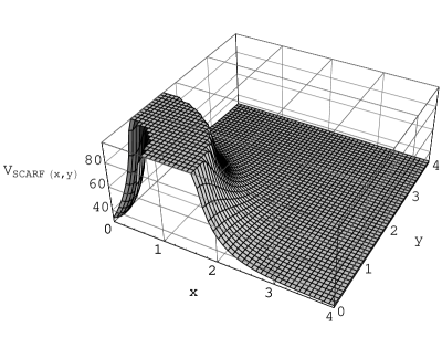
Figure 1: The q-deformed Scarf potential; $V_{0}=10,V_{1}=15,V_{2}=10,q=10,\alpha=1.$

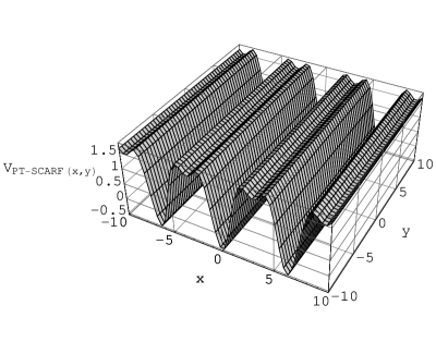
Figure 2: PT-symmetric q-deformed Scarf potential;$V_{0}=1,V_{1}=1,V_{2}=1,q=1,\alpha=1.$

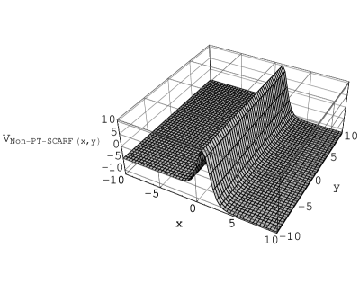
Figure 3: Non-PT-symmetric q-deformed Scarf potential;$V_{0}=10,V_{1}=15,V_{2}=10,q=10,\alpha=1.$

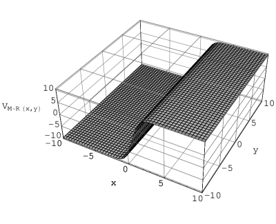
Figure 4: The Manning-Rosen potential;$A=10,B=1,q=-4,\alpha=1.$

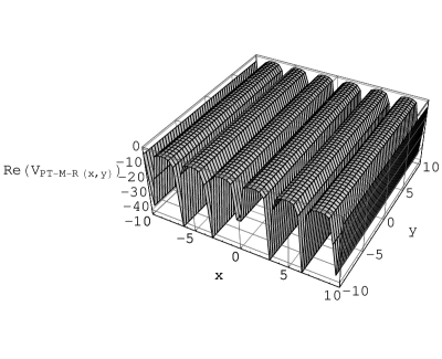
Figure 5: The real part of the PT-symmetric Manning-Rosen potential;$A=1,B=1,q=1,\alpha=1.$

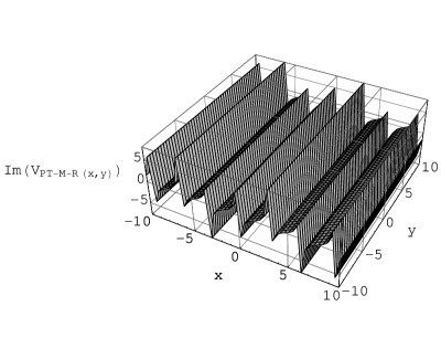
Figure 6: The imaginer part of the PT-symmetric Manning-Rosen potential;$A=1,B=1,q=1,\alpha=1.$

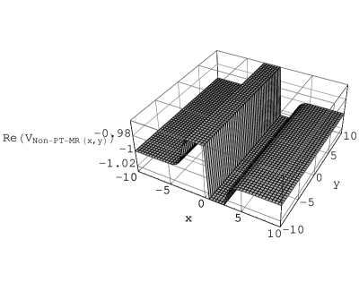
Figure 7: The real part of the Non-PT-symmetric Manning-Rosen potential;$A=1,B=1,q=1,\alpha=1.$

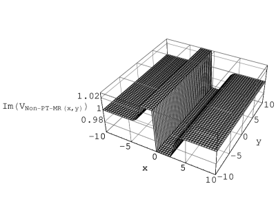
Figure 8: The imaginer part of the Non-PT-symmetric Manning-Rosen potential;$A=1,B=1,q=1,\alpha=1.$

References

• [1] C. M. Bender and S. Boettcher,   Phys. Rev. Lett. 80 (1998) 5243; C. M. Bender,  J. Math. Phys. 40 (1999) 2201;C. M. Bender,D. C. Brody, H. F. Jones,  Phys. Rev. Lett. 89 (2002) 270401; C. M. Bender, P. N. Meisinger, Q. Wang,  J. Phys. A:Math. Gen. 36 (2003) 1095;C. M. Bender,D. C. Brody, H. F. Jones,  Am. J. Phys. 71 (2003) 1095;C. M. Bender, P. N. Meisinger, Q. Wang,  J. Phys. A:Math. Gen. 36 (2003) 1029.
• [2] A. Mostafazadeh, J. Math. Phys 43 (2002) 205; ibid 43 (2002) 2814; ibid 43 (2002) 3944; J. Phys. A:Math.Gen. 36 (2003) 7081.
• [3] Z. Ahmed, Phys. Lett. A 290 (2001) 19; ibid 310 (2003) 139; J. Phys. A:Math.Gen. 36 (2003) 10325.
• [4] T. V. A. Fityo, J. Phys. A 35 (2002) 5893.
• [5] C. M. Bender, F. Cooper, P. N. Meisinger, M. V. Savage, Phys. Lett. A 259 (1999) 229.
• [6] C. M. Bender and G. V. Dunne and P. N. Meisinger, Phys. Lett. A 252 (1999) 272.
• [7] V. Buslaev and V. Grecchi, J. Phys. A 36 (1993) 5541.
• [8] E. Delabaere and F. Bham, Phys. Lett. A 250 (1998) 25; ibid 250 (1998) 29.
• [9] C. M. Bender and K. A. Milton and V. M. Savage, Phys.Rev.D 62 (2000) 085001; C. M. Bender, S. Boettcher, H. F. Jones and P. N. Meisinger, J.Math. Phys. 42 (2001) 1960.
• [10] B. Bagchi and C. Quesne, Phys. Lett. A 273 (2000) 285; B. Bagchi and C. Quesne, Phys. Lett. A 300 (2002) 18; G. Lévai, F. Cannata, A. Ventura, J. Phys. A:Math.Gen. 34 (2001) 839 ; G. Lévai, F. Cannata, A. Ventura, J. Phys. A:Math.Gen. 35 (2002) 5041.
• [11] S. Dutra, M. B. Hott and V. G. C. S. dos Santos, Europhys. Lett. 71(2) (2005) 166; U. Guenther, F. Stefani, M. Znojil, J.Math.Phys. 46 (2005) 063504.
• [12] H. Egrifes, D. Demirhan, F. Buyukkilic,  Physica Scripta 59 (1999) 90.
• [13] H. Egrifes, D. Demirhan, F. Buyukkilic,  Physica Scripta 60 (1999) 195.
• [14] H. Egrifes, D. Demirhan, F. Buyukkilic,  Theor. Chem. Acc. 98 (1997) 192.
• [15] A. F. Nikiforov, V. B. Uvarov, ”Special Functions of Mathematical Physics”, Birkhauser, Basel, 1988.
• [16] O . Yesiltas, M. Simsek, R. Sever and C. Tezcan, Physica Scripta T67 (2003) 472; M. Znojil Phys. Lett. A 264 (1999) 108 ;
• [17] M Aktas, R. Sever, Mod. Phys. Letts. A 19 (2004) 2871; H. Egrifes and R. Sever, Phys. Lett. A 344(2-4) (2005) 117-126; S. M. Ikhdair, R. Sever, ArXiv:quant-ph/0604078 ;M. Simsek, H. Egrifes, J. Phys. A: Math. Gen. 37 (2004) 4379-4393;
• [18] B. Gonul,  ArXiv:quant-ph/0604021; B. Gonul, K. Koksal and E. Bak r, Phys. Scr. 73 (2006) 279.
• [19] S. S. Ranjani, A. K. Kapoor, Annals of Physics 320 (2005) 164.
• [20] C. Grosche, J. Phys. A:Math.Gen. 38 (2005) 2947.
• [21] A. de Souza Dutra,  ArXiv:quant-ph/0501094.
Refer to caption