Effective generation of cat and kitten states

Abstract

We present an effective method of coherent state superposition (cat state) generation using single trapped ion in a Paul trap. The method is experimentally feasible for coherent states with amplitude $\alpha\leq 2$ using available technology. It works both in and beyond the Lamb-Dicke regime.

1. Introduction

One of the most inspiring aspects of quantum physics is the possibility of generation a quantum superpositions of two more macroscopic, classically distinguishable, interfering states. This idea is closely related to the famous Schrödinger cat paradox [1], where the cat is set to be alive and dead with equal probabilities until the measurement is made. This state is entangled to the device that can kill the cat. In recent literature just the superposition of two coherent states with a $\pi$ phase difference and a large amplitude inherited the name, and is referred as a cat state. A superposition of more than two coherent states is called a kitten state.

The cat and kitten states have brought a lot of interest of physicists due to many possible applications in quantum information processing [2, 3, 4, 5, 6], quantum teleportation [2, 3], quantum nonlocality tests [7, 8], generation and purification of entangled coherent states [3], and quantum computation and communication [3, 4, 5, 9]. Those states are also very useful for investigation of the decoherence process [10, 11].

So far, a superposition of two coherent states has been successfully generated for phonon modes of a single trapped ion [10] and superconducting cavity [12]. A lot of effort has been made to investigate the possibility of photon coherent state superposition generation using Kerr nonlinearity [13, 14]. However, the nonlinearity is far too small to ensure the effective method of the state preparation.

The aim of this article is to focus on the possibilities of the coherent state superposition generation, which are offered by the trapped ions in a Paul trap. The ion traps have generated a lot of interest due to their possible applications in quantum information theory [15] and quantum computation [16]. In different experiments, Fock number states [17], coherent states [18], vacuum squeezed states [19], and Schrödinger cat states [10] has been realized. According to our knowledge, neither non-Gaussian states (other than cat state) nor a superposition of more than two coherent states have been observed so far.

The presented method allows for the generation of two and more, eg. six, coherent states superposition. It is closely related to the Kerr nonlinear interaction. It is experimentally feasible for coherent states with the amplitude $\alpha\leq 2$.

2. Kerr state

Let us begin the discussion with a brief summary of a Kerr state and a Kerr medium.

The one-mode Kerr state results from an interaction of a coherent state of light $|\alpha\rangle$ with a third-order $\chi^{(3)}$ nonlinear medium, the Kerr medium [20]. The optical fibers are the best known example of the Kerr medium.

The Hamiltonian describing the interaction in the ideal medium, without damping and thermal noise, is of the following form

$$H=\hbar\frac{\kappa}{2}\,a^{\dagger}a^{\dagger}a\,a,$$ (1)

where $a$ and $a^{\dagger}$ are annihilation and creation operators of the light mode. The strength of the medium is given by the nonlinear constant $\kappa=\frac{8\pi^{2}\hbar\omega^{2}}{\epsilon_{0}n_{0}^{4}(\omega)V}\chi^{(3)}$, where $\omega$ is the frequency of the injected light beam, $n_{0}(\omega)$ is the linear refractive index and $V$ is the volume of quantization.

The one-mode Kerr state is an infinite superposition of different photon number states (Fock states)

$$|\Psi_{K}(\tau)\rangle=e^{-\frac{iHt}{\hbar}}|\alpha\rangle=e^{-\frac{|\alpha|^{2}}{2}}\sum_{n=0}^{\infty}\,\frac{\alpha^{n}}{\sqrt{n!}}\,e^{i\frac{\tau}{2}n(n-1)}|n\rangle.$$ (2)

Its properties are characterized by a dimensionless parameter $\tau=-\kappa t$, where $t$ is a time that the light has spent in the fiber.

Although the statistics of the Kerr state is Poissonian, $g^{(2)}(\tau)=1$, this is a squeezed state. This fact can be easily observed from the evolution of its electric field quadrature uncertainties

$$(\Delta X_{1})^{2} = 1+2\alpha^{2}\left(1-e^{2\alpha^{2}(\cos\tau-1)}+\mathrm{Re}\{e^{i\tau+\alpha^{2}(e^{2i\tau-1})}-e^{2\alpha^{2}(e^{i\tau-1})}\}\right),$$ (3)

$$(\Delta X_{2})^{2} = 1+2\alpha^{2}\left(1-e^{2\alpha^{2}(\cos\tau-1)}-\mathrm{Re}\{e^{i\tau+\alpha^{2}(e^{2i\tau-1})}-e^{2\alpha^{2}(e^{i\tau-1})}\}\right),$$ (4)

where $X_{1}=a+a^{\dagger}$ and $X_{2}=-i(a-a^{\dagger})$ are amplitude and phase quadratures. Depending on $\tau$, the quadratures are squeezed alternately: the quantum fluctuations in one quadrature are reduced below the vacuum level, $1$, at the expense of increased fluctuations in the other one, see Fig.1. If none of them is squeezed for a given value of $\tau$, the squeezing will not be seen in the principal axes directions but for quadratures at a certain angle. This fact corresponds to the rotation of the error contour in the phase space.

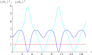
Fig. 1: (Color online) The evolution of the amplitude and the phase quadrature uncertainties, $(\Delta X_{1})^{2}$ (dark blue) and $(\Delta X_{2})^{2}$ (light blue), for $\alpha=1$. The line is a reference value of $1$ obtained for a vacuum.

The Kerr state is a non-Gaussian quantum state. This information can be obtained from its Wigner phase space function: it takes the negative values and it is not rotational symmetric. The Wigner function can be computed and expressed in two equivalent ways

$$W(\tau,\gamma,\gamma^{*}) = \frac{2}{\pi}\,e^{-2|\gamma|^{2}}e^{-|\alpha|^{2}}\,\sum_{q=0}^{\infty}\frac{\left(2\alpha^{*}\gamma e^{i\frac{\tau}{2}}\right)^{q}}{q!}e^{-i\frac{\tau}{2}q^{2}}$$ (5)

$$\times \sum_{k=0}^{\infty}\frac{\left(2\alpha\gamma^{*}e^{-i\frac{\tau}{2}}\right)^{k}}{k!}e^{i\frac{\tau}{2}k^{2}}e^{-|\alpha|^{2}e^{i\tau(k-q)}},$$

$$W(\tau,\gamma,\gamma^{*}) = \frac{2}{\pi}\,e^{2|\gamma|^{2}}e^{-|\alpha|^{2}}\,\sum_{n,m=0}^{\infty}\frac{1}{(-2)^{n+m}}\frac{\alpha^{n}}{n!}\frac{{\alpha^{*}}^{m}}{m!}$$

$$\times e^{i\frac{\tau}{2}\left[n(n-1)-m(m-1)\right]}\left(\partial_{\gamma}\right)^{n}\left(\partial_{\gamma^{*}}\right)^{m}e^{-4|\gamma|^{2}}.$$

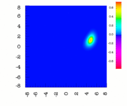
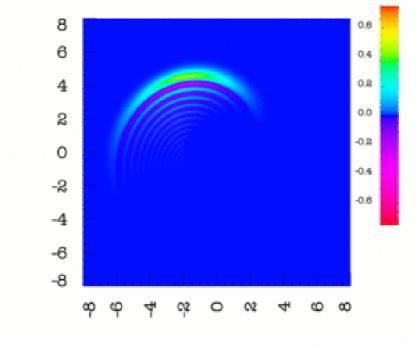
Fig. 2: (Color online) The Wigner function evaluated for $\alpha=5$. For $\tau=0.01$ the Wigner function is an ellipse and the state becomes squeezed - the left figure. The Wigner function for $\tau=0.08$ - the right figure. The negativities appear and form a tail of interference fringes.

The examples of the Wigner function evaluated for $\alpha=5$ and two values of evolution parameter $\tau=0.01$ and $\tau=0.08$ are depicted on Fig. 2. The distribution starting with a circular shape genuine to a coherent state turns into an ellipse and the state becomes squeezed - the left figure. It also shows that the Kerr state approximates a one-mode Gaussian squeezed state for $\tau\simeq 0$ very well. Then, the ellipse is stretched into a banana shape - the right figure. This plot reveals the nonclassicality of the state: the negative values of the Wigner function form a tail of interference fringes following the “main” part of the “banana” distribution.

3. Cat and kitten states

The evolution of a coherent state in a Kerr medium is periodic: the phase factor in the Kerr state (2) is a periodic function of the parameter $\tau$. Therefor, we achieve the same state for $\tau$ and $\tau+2\pi$. Moreover, if $\tau$ is taken as a fraction of the period of the evolution, $\tau=2\pi R$ where $R<1$ is a rational number, the infinite sum of Fock states breaks into a finite sum of coherent states, all of the same amplitude but different phases [21]. This effect is also known as a fractional revival [22].

Below we present the cat and kitten states - the superpositions of 2-6 coherent states - and their Wigner functions obtained from the Kerr state (2) for some specific values of $\tau$ and $\alpha=2$, Fig. 3-5.

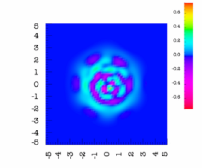
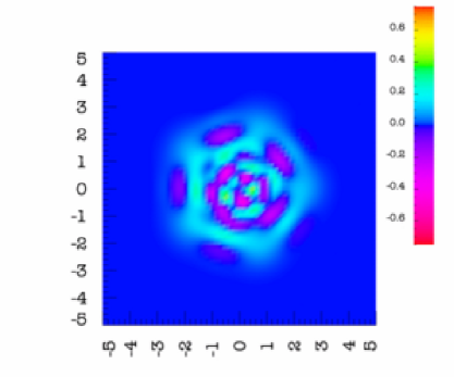
Fig. 3: (Color online) The Wigner function evaluated for $\alpha=2$. The left figure: $\tau=\frac{\pi}{3}$. The Kerr state becomes a superposition of six coherent states: $|2e^{i\frac{\pi}{6}}\rangle$, $|2e^{i\frac{\pi}{2}}\rangle$, $|2e^{i\frac{5\pi}{6}}\rangle$, $|2e^{i\frac{7\pi}{6}}\rangle$, $|2e^{i\frac{3\pi}{2}}\rangle$, $|2e^{i\frac{11\pi}{6}}\rangle$. The right figure: $\tau=\frac{2\pi}{5}$. The Kerr state becomes a superposition of five coherent states: $|2\rangle$, $|2e^{i\frac{2\pi}{5}}\rangle$, $|2e^{i\frac{4\pi}{5}}\rangle$, $|2e^{i\frac{6\pi}{5}}\rangle$, $|2e^{i\frac{8\pi}{5}}\rangle$.

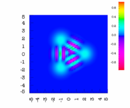
Fig. 4: (Color online) The Wigner function evaluated for $\alpha=2$. The left figure: $\tau=\frac{\pi}{2}$. The Kerr state becomes a superposition of four coherent states: $|2e^{i\frac{\pi}{4}}\rangle$, $|2e^{i\frac{3\pi}{4}}\rangle$, $|2e^{i\frac{5\pi}{4}}\rangle$, $|2e^{i\frac{7\pi}{4}}\rangle$. The right figure: $\tau=\frac{2\pi}{3}$. The Kerr state becomes a superposition of three coherent states: $|2\rangle$, $|2e^{i\frac{2\pi}{3}}\rangle$, $|2e^{i\frac{4\pi}{3}}\rangle$.

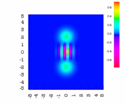
Fig. 5: (Color online) The Wigner function evaluated for $\alpha=2$ and $\tau=\pi$. The Kerr state becomes a superposition of two coherent states: $|2e^{i\frac{\pi}{2}}\rangle$, $|2e^{i\frac{3\pi}{2}}\rangle$.

Setting $\tau=\frac{\pi}{3}$ the Kerr state becomes a superposition of six coherent states

$$|\Psi_{K}(\tau=\frac{\pi}{3})\rangle = c_{1}|2e^{i\frac{\pi}{6}}\rangle+c_{2}|2e^{i\frac{\pi}{2}}\rangle+c_{3}|2e^{i\frac{5\pi}{6}}\rangle$$ (7)

$$+ c_{2}|2e^{i\frac{7\pi}{6}}\rangle+c_{1}|2e^{i\frac{3\pi}{2}}\rangle+c_{4}|2e^{i\frac{11\pi}{6}}\rangle,$$

with the following coefficients: $c_{1}=\frac{1}{6}\left(2+2i+e^{-i\frac{\pi}{6}}+e^{-i\frac{2\pi}{3}}\right)$, $c_{2}=\frac{1}{6}\left(2-2i+e^{i\frac{5\pi}{6}}+e^{-i\frac{2\pi}{3}}\right)$, $c_{3}=\frac{1}{6}\left(1+i+2e^{-i\frac{5\pi}{6}}+2e^{i\frac{2\pi}{3}}\right)$, $c_{4}=\frac{1}{6}\left(1-i+2e^{i\frac{\pi}{6}}+2e^{i\frac{2\pi}{3}}\right)$.

We have five coherent states for $\tau=\frac{2\pi}{5}$

$$|\Psi_{K}(\tau=\frac{2\pi}{5})\rangle = c_{1}|2\rangle+c_{2}|2e^{i\frac{2\pi}{5}}\rangle+c_{3}|2e^{i\frac{4\pi}{5}}\rangle+c_{2}|2e^{i\frac{6\pi}{5}}\rangle+c_{1}|2e^{i\frac{8\pi}{5}}\rangle,$$ (8)

where $c_{1}=\frac{1}{5}\left(2+2e^{i\frac{2\pi}{5}}+e^{-i\frac{4\pi}{5}}\right)$, $c_{2}=\frac{1}{5}\left(2+2e^{-i\frac{2\pi}{5}}+e^{i\frac{4\pi}{5}}\right)$, $c_{3}=\frac{1}{5}\left(1+2e^{i\frac{4\pi}{5}}+2e^{-i\frac{4\pi}{5}}\right)$.

For $\tau=\frac{\pi}{2}$ we have superposition of four states

$$|\Psi_{K}(\tau=\frac{\pi}{2})\rangle = c_{1}|2e^{i\frac{\pi}{4}}\rangle+c_{2}|2e^{i\frac{3\pi}{4}}\rangle+c_{1}|2e^{i\frac{5\pi}{4}}\rangle-c_{2}|2e^{i\frac{7\pi}{4}}\rangle,$$ (9)

with $c_{1}=\frac{1}{4}\left(2+e^{-i\frac{\pi}{4}}+e^{i\frac{3\pi}{4}}\right)$, $c_{2}=\frac{1}{2}e^{-i\frac{3\pi}{4}}$.

If $\tau=\frac{2\pi}{3}$ the Kerr state becomes superposition of three states

$$|\Psi_{K}(\tau=\frac{2\pi}{3})\rangle = c_{1}|2\rangle+c_{2}|2e^{i\frac{2\pi}{3}}\rangle+c_{1}|2e^{i\frac{4\pi}{3}}\rangle,$$ (10)

where $c_{1}=\frac{1}{3}\left(2+e^{i\frac{2\pi}{3}}\right)$, $c_{2}=\frac{1}{3}\left(1+2e^{-i\frac{2\pi}{3}}\right)$.

We achieve the usual cat state, the superposition of two coherent states, for $\tau=\pi$

$$|\Psi_{K}(\tau=\pi)\rangle = \frac{1}{2}(1-i)|2e^{i\frac{\pi}{2}}\rangle+\frac{1}{2}(1+i)|2e^{i\frac{3\pi}{2}}\rangle.$$ (11)

4. Approximated cat and kitten state generation using ion traps

All the presented kitten states (7) - (11) can be generated using current technology available for the ion traps and already existing theoretical schemes for an ion arbitrary pure state preparation, if the amplitude of the coherent state is not too large.

We show that the small kitten states can be very well approximated by a superposition of only few Fock states with appropriate chosen coefficients. It means that only a small number of Fock states in Eq. (2) is of real significance and the sum can be cut off at some $n=M$. We analyze the dependence of this number $M$ on the initial coherent state amplitude $\alpha$.

A method of preparing an ion in a Paul trap [23] in a finite superposition of Fock states with arbitrary coefficients

$$|\Psi^{(M)}\rangle_{\mathrm{ion}}=\sum_{n=0}^{M}c_{n}|n\rangle|g\rangle,$$ (12)

has been proposed in [24, 25]. In the above formula $|n\rangle$ is an ion motional Fock state, defined according to a harmonic oscillator potential in the trap, $M<\infty$. The states $|g\rangle$ and $|e\rangle$ are the ion electronic ground and excited states. The method is based on applying a series of laser pulses tuned to the carrier frequency and the red sideband of the ion trap alternately. It works both in and beyond the Lamb-Dicke regime.

Adjusting the time of laser pulses or their Rabi frequency we can obtain

$$c_{n}=\frac{1}{\sqrt{\sum_{k=0}^{M}\frac{|\alpha|^{2k}}{k!}}}\frac{\alpha^{n}}{\sqrt{n!}}\,e^{i\frac{\tau}{2}n(n-1)}.$$ (13)

In that case we generate the approximated cat state applying $2M$ laser pulses

$$|\Psi_{K}^{(M)}(\tau)\rangle=R_{M}C_{M-1}\cdot...\cdot C_{1}R_{1}C_{0}|0,g\rangle.$$ (14)

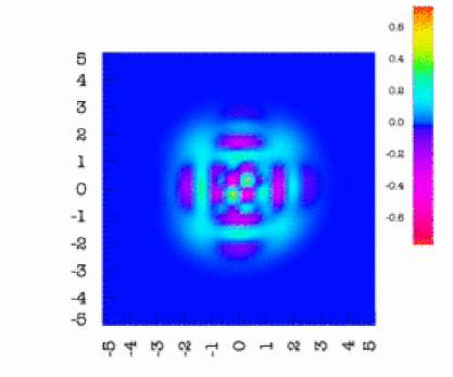
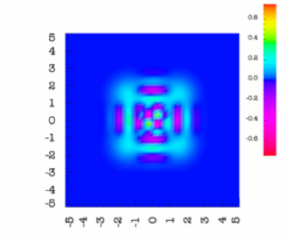
Fig. 6: (Color online) The Wigner function evaluated for $\alpha=2$ and $\tau=\frac{\pi}{2}$. The left figure: $M=10$. The right figure: $M=30$.

The choice of the value $M$ of the cut off in the sum (2) is based on comparison of the Wigner function computed for different values of $M$. On Fig. 6 we present the Wigner function evaluated for $M=10$ and $M=30$ for $\alpha=2$ and $\tau=\frac{\pi}{2}$. Please note, that there is no significant difference between the left and right figure. We have also checked that $M=5$ simplifies the Wigner function too much, Fig. 7.

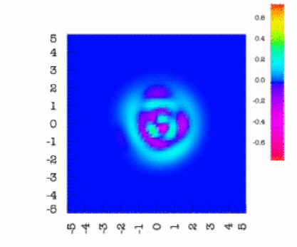
Fig. 7: (Color online) The Wigner function evaluated for $\alpha=2$, $\tau=\frac{\pi}{2}$ and $M=5$.

Therefor, we assume that $|\Psi_{K}^{(10)}(\tau)\rangle$ approximates the cat state for $\alpha=2$ good enough, which means that $20$ laser pulses are required for its preparation.

The appropriate value of $M$ is approximately equal to the number of significant number of coefficients in the sum (2). Below we present the plots of absolute values of $c_{n}$, Eq. (13), as a function of $n$ for $\alpha=1$, $\alpha=2$ and $\alpha=5$. The number of the laser pulses required for the kitten state preparation increases with the magnitude of the amplitude $\alpha$ fast.

Fig. 8: The absolute values of $c_{n}$, Eq. (13), as a function of $n$ for $\alpha=1$ - the left figure, $\alpha=2$ - the middle figure and $\alpha=5$ - the right figure.

The value of the amplitude eg. $\alpha=5$ requires about $100$ pulses and the decoherence effects would have to be compensated for during the preparation. Such an amplitude also requires higher number states in Eq. (2) that have to be taken into account, which means dealing with higher excitations of ion.

As an example, we list below the set of laser pulses parameters required for approximated kitten state $|\Psi^{(10)}_{K}(\tau=\frac{\pi}{2})\rangle_{\mathrm{ion}}$ for $\alpha=2$ generation.

Assuming the carrier resonance Rabi frequency (for all pulses $C_{i}$) equal to $\Omega_{C}=1\mathrm{MHz}$ and the red sideband Rabi frequency (for all pulses $R_{i}$) equal to $\Omega_{R}=100\mathrm{kHz}$, the duration times and phases of pulses are as follows

$$\begin{array}[]{rllrll}R10:&\phi=\pi,&t_{10}^{R}=995\mu\mathrm{s};&C9:&\phi=0,&t_{9}^{C}=2.89\mu\mathrm{s},\\ R9:&\phi=0.47,&t_{9}^{R}=387\mu\mathrm{s};&C8:&\phi=-0.83,&t_{8}^{C}=1.16\mu\mathrm{s},\\ R8:&\phi=7.23,&t_{8}^{R}=351\mu\mathrm{s};&C7:&\phi=1.33,&t_{7}^{C}=1.30\mu\mathrm{s},\\ R7:&\phi=4.26,&t_{7}^{R}=435\mu\mathrm{s};&C6:&\phi=2.41,&t_{6}^{C}=2.21\mu\mathrm{s},\\ R6:&\phi=5.00,&t_{6}^{R}=474\mu\mathrm{s};&C5:&\phi=-0.05,&t_{5}^{C}=1.60\mu\mathrm{s},\\ R5:&\phi=1.82,&t_{5}^{R}=546\mu\mathrm{s};&C4:&\phi=-0.86,&t_{4}^{C}=2.44\mu\mathrm{s},\\ R4:&\phi=2.21,&t_{4}^{R}=550\mu\mathrm{s};&C3:&\phi=-2.97,&t_{3}^{C}=1.92\mu\mathrm{s},\\ R3:&\phi=-1.30,&t_{3}^{R}=745\mu\mathrm{s};&C2:&\phi=-3.93,&t_{2}^{C}=2.84\mu\mathrm{s},\\ R2:&\phi=-0.95,&t_{2}^{R}=813\mu\mathrm{s};&C1:&\phi=-0.09,&t_{1}^{C}=2.84\mu\mathrm{s},\\ R1:&\phi=3.23,&t_{1}^{R}=1370\mu\mathrm{s};&C0:&\phi=-4.19,&t_{0}^{C}=1.04\mu\mathrm{s}.\end{array}$$

We could also keep the duration time of pulses constant, $t_{C}=t_{R}=1\mu\mathrm{s}$, and change the Rabi frequencies from pulse to pulse

$$\begin{array}[]{rllrll}R10:&\phi=\pi,&\Omega_{10}^{R}=94.9\mathrm{MHz};&C9:&\phi=0,&\Omega_{9}^{C}=2.89\mathrm{MHz},\\ R9:&\phi=0.47,&\Omega_{9}^{R}=36.7\mathrm{MHz};&C8:&\phi=-0.83,&\Omega_{8}^{C}=1.16\mathrm{MHz},\\ R8:&\phi=7.23,&\Omega_{8}^{R}=33.1\mathrm{MHz};&C7:&\phi=1.33,&\Omega_{7}^{C}=1.30\mathrm{MHz},\\ R7:&\phi=4.26,&\Omega_{7}^{R}=40.7\mathrm{MHz};&C6:&\phi=2.41,&\Omega_{6}^{C}=2.21\mathrm{MHz},\\ R6:&\phi=5.00,&\Omega_{6}^{R}=43.9\mathrm{MHz};&C5:&\phi=-0.05,&\Omega_{5}^{C}=1.60\mathrm{MHz},\\ R5:&\phi=1.82,&\Omega_{5}^{R}=49.9\mathrm{MHz};&C4:&\phi=-0.86,&\Omega_{4}^{C}=2.44\mathrm{MHz},\\ R4:&\phi=2.21,&\Omega_{4}^{R}=49.1\mathrm{MHz};&C3:&\phi=-2.97,&\Omega_{3}^{C}=1.92\mathrm{MHz},\\ R3:&\phi=-1.30,&\Omega_{3}^{R}=64.5\mathrm{MHz};&C2:&\phi=-3.93,&\Omega_{2}^{C}=2.84\mathrm{MHz},\\ R2:&\phi=-0.95,&\Omega_{2}^{R}=66.4\mathrm{MHz};&C1:&\phi=-0.09,&\Omega_{1}^{C}=2.84\mathrm{MHz},\\ R1:&\phi=3.23,&\Omega_{1}^{R}=96.9\mathrm{MHz};&C0:&\phi=-4.19,&\Omega_{0}^{C}=1.04\mathrm{MHz}.\end{array}$$

The phases will not change. As an initial state we take $|\phi_{in}\rangle=(-0.97+0.25i)|0,g\rangle$ and the Lamb-Dicke parameter $\eta=0.02$.

5. Conclusion

In this paper we have presented a method of an effective approximated coherent superposition state generation for a single trapped ion in a Paul trap.

At first, the ion is prepared in its ground state, both in motional and electronic state. Then, step by step, the state is built up applying a series of laser pulses tuned to the carrier resonance and red sideband interaction alternately.

Fixing the amplitude of the coherent state, we can approximate the cat state arbitrary well, increasing the number of applied pulses.

The cat and kitten states with their amplitude $\alpha\leq 2$ are very well approximated by a state which is available applying $20$ laser pulses. The judgment is based on a Wigner function comparison.

References

- [1] E. Schrödinger, Naturwissenschaften, 23, 807 (1935).
- [2] S. J. van Enk and O. Hirota, Phys. Rev. A, 64, 022313 (2001).
- [3] H. Jeong, M. S. Kim, and J. Lee, Phys. Rev. A, 64, 052308 (2001).
- [4] H. Jeong and M. S. Kim, Phys. Rev. A, 65, 042305 (2002).
- [5] T. C. Ralph, A. Gilchrist, G. J. Milburn, W. J. Munro and S. Glancy, Phys. Rev. A 68, 042319 (2003).
- [6] T. C. Ralph, Phys. Rev. A, 65, 042313 (2002).
- [7] H. Jeong et al., Phys. Rev. A, 67, 012106 (2003).
- [8] V. Buzek et al., Phys. Rev. A, 45, 6570 (1992).
- [9] S. Glancy, H. M. Vasconcelos, and T. C. Ralph, Phys. Rev. A, 70, 022317 (2004).
- [10] C. Monroe, D. Meekhof, B. E. King, and D. J. Wineland, Science, 272, 1131 (1996).
- [11] Myatt et. al, Nature 403, 269 (2000).
- [12] M. Brune et al., Phys. Rev. Lett., 77, 4887 (1996).
- [13] H. Jeong, M. S. Kim, T. C. Ralph, and B. S. Ham, Phys. Rev. A, 70, 061801(R) (2004).
- [14] M. Stobińska, G. J. Milburn, K. Wódkiewicz, quant-ph/0605166.
- [15] R. Blatt and A. Steane, Quantum Information Processing and Communication in Europe, pp. 161-169, European Communities (2005).
- [16] A. Ekert and Josza, Rev. Mod. Phys. 68, 733 (1996).
- [17] Ch. Roos et al., Phys. Rev. Lett. 83, 4713 (1999).
- [18] D. M. Meekhof et al., Phys. Rev. Lett. 76, 1796 (1996).
- [19] D. J. Heinzen and D. J. Wineland, Phys. Rev. A 42, 2977 (1990).
- [20] R. Tanaś, Nonclassical states of light propagating in Kerr media, in Theory of Non-Classical States of Light, V. Dodonov and V. I. Man’ko eds., Taylor and Francis, London 2003.
- [21] Z. Bialynicka-Birula, Phys. Rev. 173, 1207 (1968).
- [22] I. Sh. Averbukh and N. F. Perelman, Phys. Lett. 139, 449 (1989).
- [23] D. Leibfried, R. Blatt, C. Monroe, and D. Wineland, Rev. Mod. Phys. 75, 281 (2003).
- [24] S. A. Gardiner, J. I. Cirac, and P. Zoller, Phys. Rev. A 55, 1683 (1997).
- [25] B. Kneer and C. K. Law, Phys. Rev. A 57, 2096 (1998).