Coupled cavity QED for coherent control of photon transmission:
Green function approach for hybrid systems with two-level doping

Abstract

This paper theoretically studies the coherent control of photon transmission along the coupled resonator optical waveguide (CROW) by doping artificial atoms in hybrid structures. We provide the several approaches correspondingly based on the mean field method and spin wave theory et al . In the present paper we adopt the two-time Green function approach to study the coherent transmission photon in a CROW with homogeneous couplings, each cavity of which is doped by a two-level artificial atom. We calculate the two-time correlation function for photon in the weak-coupling case. Its poles predict the exact dispersion relation, which results in the group velocity coherently controlled by the collective excitation of the doping atoms. We emphasize the role of the population inversion of doping atoms induced by some polarization mechanism.

I Introduction

Recently, all-optical and on-chip setups with the coupled resonator optical waveguide (CROW) have been implemented experimentally to show the coherent transmission of “slow photons” Fanprl06 ; nat441 , which is similar to the electromagnetical induced transparency (EIT) effect EIT97 ; EIT01 occurring in the atomic ensemble medium. This successful experiment implies the coherent couplings of the single mode cavities Fanprl04 , which result in the photonic-crystal-like system with photonic band structure. For practical applications such as CROW setup they can be utilized to stop or store the light pulses propagation and then lead to a quantum device based on these many-body effects, which can also be regarded as a tunable quantum simulator for the tight binding fermion system in condensed matter physics.

On the other hand, recently it was discovered Bqp06159 ; Pqp06097 that, when such an array of coupled cavities is doped with two-level atoms, the photon-blockaded phenomenon can emerge and achieve a Mott insulator state of polaritons that are many-body dressed states of doped atoms coupled to quantized modes of optical field in the CROW. Most interestingly, such a hybrid system with a two-dimensional array of coupled optical cavities in the photon-blockaded regime will undergo a quantum phase transition from characteristic Mott insulator (excitations localized on each site) to superfluid (excitations delocalized across the lattice) lqpt . A similar coplanar hybrid structure based on superconducting circuit has been proposed for the coherent control of microwave-photons propagating in a coupled transmission line resonator (CTLR) waveguide. Here, each cavity is coupled to a tunable charge qubit sup . While the CTLR forms an artificial photonic crystal with an engineered band structure, the charge qubits collectively behave as spin waves in the low-excitation limit, and these charge qubits modify the photonic band with energy gaps to slow or even stop the microwave propagation in this CTLR waveguide. The conceptual exploration here suggests an electromagnetically controlled quantum device based on the on-chip circuit for the coherent manipulation of photons, such as the dynamic appearances of the laser-like output from CTLR waveguide where the atoms are pumped for some population inversion.

These progressing investigations motivate us to further develop the general theoretical approach for cavity quantum electrodynamics (QED) with coupled resonators for coherent manipulations of photon transmission in an artificial photonic band structure, which can be controlled through some new mechanisms. In Ref.zhou we provide an approach based on the mean filed method and spin wave theory et al for different hybrid structures, which consist of the coupled cavity arrays with homogeneous (or inhomogeneous) couplings and various multi-level-atom doping.

The present paper adopts the two-time Green function approach to study the coherent transmission of photons in a CROW with homogeneous couplings, each cavity is doped to a two-level artificial atom. Mathematically the hybrid system has the same model as that for CTLR waveguide connected to charge qubitssup , but the Green function can work well for the system which does not satisfy the low-excitation limit, in which we can even obtain exact solution sunprl91 . We calculate the two-time retarded Green function for photons in the weak-coupling case. Its poles predict the exact dispersion relation, according to which the group velocity can be coherently controlled by the collective excitation of the doping atoms. We emphasize the role of the population inversion of the total doping atoms, which is induced by some polarization or pump mechanism. The dispersion relation exhibits some exotic features such as the compressed photonic bandwidth.

The paper is organized as followed. In section II we describe our setup of the photonic band device CROW interacting with doping atoms. Applying the retarded two-time Green function theory, in section III, we calculate the eigenfrequencies of the hybrid photon-atom system to characterize the coherent features of photon transmission. In section IV we study how the bandwidth and group velocity of photon transmission can be adjusted by controlling the doped atoms. Then we consider the effects of damping in both the local mode of cavity and doped atoms. The stable atomic collective excitations can result in the coherent output of slow photons with some laser-like properties. In section V, for the phenomenon of slow photons we study the effective susceptibility of light propagation in the CROW interacting with doping atoms. In the appendices we give some necessary details for the Green function calculations and analyze the quasi-spin wave structure represented by the Green functions for photons and atoms that we have obtained.

II Model for hybrid structure with photonic bands

We consider a hybrid structure (illustrated in Fig.1 a )- the coupled cavity array with doping artificial atoms. Here, $N$ optical cavities with homogeneous and nearest-neighbor couplings form a one-dimensional periodic structure, which is similar to the fermion system on tight binding lattice. In practice, there are two ways to implement such CROW. 1. With photonic crystals, the coupled cavities are built through regularly breaking the periodicity of photonic crystal. In the photonic bandgap materials, the cavities are defined by an array (superlattice) of periodic defects in the periodic modulation. The inter-cavity hopping of photons is due to overlap between two cavity mode functions. 2. In an electromagnetically controlled quantum device based on superconducting circuit sup , the CROW is realized by the superconducting waveguide with coupled transmission line resonators, while the doping systems are implemented by the biased Cooper pair boxes.

Figure 1: (Color online)Configuration of controlled light propagation in a coupled resonator optical waveguide (CROW) by doping a two-level system (a). To implement a controllable Rabi transition between the excited and ground states of the effective two-level system (b), the stimulated Ramann mechanism is used for a three-level system (c) where the classical controlling light is resonant between the auxiliary level and the excited level.

In Fig.1 (b, c), to implement a Rabi transition with controllable coupling between the excited state $|e_{\alpha}\rangle$ and ground state $|g_{\alpha}\rangle$ of the doping two-level system with level spacing $\omega_{A}$, the stimulated Ramann mechanism is usually used for a three-level system where the classical controlling light is resonant between the auxiliary level $|f_{\alpha}\rangle$ and the excited level $|e_{\alpha}\rangle$.

Actually, for the sake of conceptual simplicity, here we assume that atom in each cavity only has three energy levels, two metastable lower states $|g_{\alpha}\rangle$, $|e_{\alpha}\rangle$ and an auxiliary state $|f_{\alpha}\rangle.$ The transition $|f_{\alpha}\rangle\rightarrow|g_{\alpha}\rangle$ is coupled to a quantized radiation mode with Rabi-frequency $\Omega,$ the frequency $\omega_{C}$ and the creation (annihilation) operator $\hat{a}_{\alpha}^{{\dagger}}$ ($\hat{a}_{\alpha}$) is in $\alpha th$ cavity, while the transitions $|f_{\alpha}\rangle\rightarrow|e_{\alpha}\rangle$ are driven by a classical controlling field with Rabi-frequency $\Omega_{c}$. Moreover, we also assume that the detuning $\Delta$ between $|g_{\alpha}\rangle$ and $|f_{\alpha}\rangle$ with respect to the quantized light is the same as that between $|g_{\alpha}\rangle$ and $|e_{\alpha}\rangle$ with respect to the classical light. Due to the stimulated Ramann effect for large detuning $\Delta$, the effective coupling can be obtained as $g=\Omega\Omega_{c}^{\ast}/\Delta$. In this sense, the effective coupling strength $g$ can be well controlled by classical Rabi-frequency $\Omega_{c}$ and the detuning $\Delta.$

To describe the collective excitations of the doping atoms, we use the quasi-spin operators

$$\sigma_{\alpha}^{z} =|e_{\alpha}\rangle\langle e_{\alpha}|-|g_{\alpha}\rangle\langle g_{\alpha}|\text{,}$$ (1)

$$\sigma_{\alpha}^{+} =|e_{\alpha}\rangle\langle g_{\alpha}|\text{,}\ \sigma_{\alpha}^{-}=|g_{\alpha}\rangle\langle e_{\alpha}|$$

to express the Hamiltonian $H=H_{A}+H_{AC}+H_{C}$ of the hybrid system. Here,

$$H_{A}=\sum_{\alpha=0}^{N-1}\frac{\omega_{A}}{2}\sigma_{\alpha}^{z}$$ (2)

is the free Hamiltonian of the doping atoms and the interaction between the local atoms and the corresponding cavity model is of Jaynes-Cummings type

$$H_{AC}=g\sum\limits_{\alpha=0}^{N-1}\hat{a}_{\alpha}\sigma_{\alpha}^{+}+h.c..$$ (3)

It shows a dynamic process that photons are absorbed when atoms transit from ground state to excited state while the photons are emitted when the atoms transit from exited state to ground state. The CROW is described by the Hamiltonian

$$H_{C}=\sum_{\alpha=0}^{N-1}\omega_{C}\hat{a}_{\alpha}^{{\dagger}}\hat{a}_{\alpha}+J\sum\limits_{\alpha=0}^{N-1}\hat{a}_{\alpha}^{{\dagger}}\hat{a}_{\alpha+1}+h.c.\text{,}$$ (4)

where $J$ denotes the inter-cavity coupling. The second term of $H_{C}$ presents the tunneling of photons from the $\alpha th$ cavity to the $\alpha+1th$ one. We notice that the model we adopt above has been used to demonstrate the photon-blockaded effect most recentlyBqp06159 ; Pqp06097 , and the lasing behavior of the output in line resonators (CTLRs) by connecting each cavity to a tunable charge qubit in circuit QEDsup .

To consider the physical significance implied by $H=H_{A}+H_{AC}+H_{C}$, we perform Fourier transformations

$$\sigma_{k}^{+} =\sum_{\alpha=0}^{N-1}\frac{e^{ik\ell\alpha}}{\sqrt{N}}\sigma_{\alpha}^{+},$$

$$\sigma^{z} =\sum_{\alpha=0}^{N-1}\frac{\sigma_{\alpha}^{z}}{N},$$ (5)

for  $k=2\pi n/(\ell N),n=0,1,...,N-1$, with the periodic boundary condition for the quasi-spin operators $\sigma_{k}^{+},$ $\sigma_{k}^{-}=(\sigma_{k}^{+})^{{\dagger}}$ and $\sigma^{z}$. The above Fourier transformation describes the collective excitations of the spatially distributed doping atoms as the quasi-spin wave via the collective operators $\sigma_{k}^{+}$ and $\sigma^{z}$ sunprl91 . This is because

$$\sigma_{k}^{+}|G\rangle=\sum_{\alpha=0}^{N-1}\frac{1}{\sqrt{N}}e^{ik\ell\alpha}|E_{\alpha}\rangle\text{,}$$ (6)

represents a spin wave where $|G\rangle=|g_{0}g_{1}g_{2}...g_{N-1}\rangle$ means all atoms are prepared in a ground state, while

$$|E_{\alpha}\rangle=|g_{0}g_{1}...g_{\alpha-1}e_{\alpha}g_{\alpha+1}...g_{N-1}\rangle\text{,}$$

means a single particle excitation in the site $\alpha$.

In order to study the collective excitation described by $\sigma_{k}^{(\pm)}$ and $\sigma^{z},$ we consider the corresponding commutation relations

$$\left[\sigma_{k}^{+},\sigma_{k^{\prime}}^{-}\right] =\sigma_{kk^{\prime}}^{z},\left[\sigma_{k}^{+},\sigma_{k}^{-}\right]=\sigma^{z},$$

$$\left[\sigma^{z},\sigma_{k}^{+}\right] =\frac{2}{N}\sigma_{k}^{+},$$

$$\left[\sigma^{z},\sigma_{k}^{-}\right] =-\frac{2}{N}\sigma_{k}^{-}\text{,}$$ (7)

where

$$\sigma_{kk^{\prime}}^{z}=\frac{1}{N}\sum_{\alpha=0}^{N-1}e^{-i(k^{\prime}-k)\ell\alpha}\sigma_{\alpha}^{z}\text{,}$$ (8)

means that $\sigma_{00}^{z}=\sigma^{z}$ , $\sigma_{k}^{+}$ and $\sigma_{k}^{-}=(\sigma_{k}^{+})^{{\dagger}}$ can not generate a $SU(2)$ subalgebra except for the case of $k=0.$ Thus $\sigma_{k}^{+}$ and $\sigma_{k^{\prime}}^{-}$  can not be regarded as a collective angular momentum for finite $N$.

Applying a discrete Fourier transformation in the $k$-space representation $\hat{a}_{k}=\sum_{\alpha}e^{ik\ell\alpha}\hat{a}_{\alpha}/\sqrt{N}$ to the Hamiltonian $H_{C}$, we have

$$H = \sum_{k=0}^{N-1}\Omega_{k}\hat{a}_{k}^{\dagger}\hat{a}_{k}+N\omega_{A}\frac{\sigma^{z}}{2}$$

$$+g\sum_{k=0}^{N-1}(\hat{a}_{k}\sigma_{k}^{+}+h.c.)\text{.}$$

The photonic band structure is characterized by the dispersion relation

$$\Omega_{k}=\omega_{C}+2J\cos(k\ell)\text{.}$$ (10)

In principle the above hybrid model can not be solved exactly, but we have analytically studied its realization based on superconducting circuit sup when few atoms are populated in their excited state - the low-excitation limit. In this case this model will be reduced to an exactly solvable coupling boson model as well as that of all-optical setup for stopping the light propagating in a CROW in Ref. Fanprl04 . The crucial issue of this observation is to use the collective operators sunprl91 $\sigma_{k}^{-}$ and $\ \sigma_{k}^{+}$ as bosonic spin wave operators in the large $N$ limit with low excitations, since the usual bosonic commutation relation $\left[\sigma_{k}^{-},\sigma_{k^{\prime}}^{+}\right]=\delta_{kk^{\prime}}$ can be approached as $N\rightarrow\infty$. However, the low excitation requires $\langle\sum_{k}\sigma_{k}^{+}\sigma_{k}^{-}\rangle\ll N$, which limits the exploitation for the general cases. So we need to develop a new technique to deal with the general cases.

III Two-time retarded Green function approach for photon transport in coupled cavity array

For quantum many-body problem, the quantum or thermal fluctuations near thermal equilibrium may be characterized by time correlation functions of the type $\ \left\langle A(t)B(t^{\prime})\right\rangle$, or by the Fourier transformations of these correlation functions, which give the correlation fluctuation spectrum. In Heisenberg picture, the time correlation function $\left\langle A(t)B(t^{\prime})\right\rangle$ of two observable$\ A$ and $B$ depends only on the time interval $t-t^{\prime}$ by the invariant of time translation. The propagation of photons in our hybrid system can be obtained by solving Green function equation for photons.

We consider the linear response of the Green function with respect to an effective applied driving force, the coupling with doping atoms. We define the two-time retarded Green function $G_{AB}^{R}\left(t,t^{\prime}\right)=\langle\langle A(t);B(t^{\prime})\rangle\rangle$ zub1960 as

$$\langle\langle A(t);B(t^{\prime})\rangle\rangle=-i\theta(t-t^{\prime})\left\langle\left[A(t),B(t^{\prime})\right]\right\rangle\text{,}$$ (11)

where $\theta(t)=1$ for $t>0$, and $\theta(t)=0$ for $t<0$.

To obtain the equation of motion for Green function, we first list the equations of motion for the creation and annihilation operators of photons and atoms by using the Hamiltonian defined in Eq. (II). Then we have the equations of motion for $G_{AB}^{R}\left(t,t^{\prime}\right)$

$$\frac{d}{dt}\langle\langle A(t);B(t^{\prime})\rangle\rangle =-i\delta(t-t^{\prime})\langle[A,B]\rangle$$

$$-i\langle\langle[A,H];B(t^{\prime})\rangle\rangle,$$ (12a)

$$\frac{d}{dt^{\prime}}\langle\langle A(t);B(t^{\prime})\rangle\rangle =i\delta(t-t^{\prime})\langle[A,B]\rangle$$

$$-i\langle\langle A(t);[B,H]\rangle\rangle.$$ (12b)

After applying the Fourier transformation from the time-domain to the frequency-domain, the retarded Green function is represented as

$$\left\langle\left\langle A|B\right\rangle\right\rangle_{\omega+i\varepsilon}=\int dte^{i(\omega+i\varepsilon)(t-t^{\prime})}\left\langle\left\langle A(t);B(t^{\prime})\right\rangle\right\rangle,$$ (13)

where $\varepsilon=+0$ is a positive infinitesimal. The equations of motion for the Green functions can be evaluated in frequency representation

$$\omega\langle\langle A|B\rangle\rangle_{\omega} =\langle[A,B]\rangle+\langle\langle[A,H]|B\rangle\rangle_{\omega},$$ (14a)

$$\omega\langle\langle A|B\rangle\rangle_{\omega} =\langle[A,B]\rangle-\langle\langle A|[B,H]\rangle\rangle_{\omega}.$$ (14b)

We notice that in the linear response theory, $$\langle\langle A|B\rangle\rangle_{\omega} \langle\langle A|B\rangle\rangle_{\omega}$$ determines the basic spectrum structure of the hybrid system through the poles of - the physical eigenfrequencies.

With the notations above, we write down the equation of the Green functions $\langle\langle\hat{a}_{k}|\hat{a}_{k}^{{\dagger}}\rangle\rangle_{\omega}$, $\langle\langle\sigma_{k^{\prime}}^{-}|\sigma_{k}^{+}\rangle\rangle_{\omega}$, $\langle\langle\sigma_{k}^{-}|\sigma_{k}^{+}\rangle\rangle_{\omega}$, $\langle\langle\hat{a}_{k}|\sigma_{k^{\prime}}^{+}\rangle\rangle_{\omega}$, and $\langle\langle\sigma_{k}^{-}|\hat{a}_{k^{\prime}}^{{\dagger}}\rangle\rangle_{\omega}$. The photon correlation $\langle\langle\hat{a}_{k}|\hat{a}_{k}^{{\dagger}}\rangle\rangle_{\omega}$ can be obtained by using the commutation relation between $\hat{a}_{k}$ and $H$ as

$$(\omega-\Omega_{k})\langle\langle\hat{a}_{k}|\hat{a}_{k}^{{\dagger}}\rangle\rangle_{\omega}=1+g\langle\langle\sigma_{k}^{-}|\hat{a}_{k}^{{\dagger}}\rangle\rangle_{\omega}.$$ (15)

We can also calculate the Green function  of the many-atom correlation $\langle\langle\sigma_{k^{\prime}}^{-}|\sigma_{k}^{+}\rangle\rangle_{\omega}$, which satisfies

$$\omega\langle\langle\sigma_{k^{\prime}}^{-}|\sigma_{k}^{+}\rangle\rangle_{\omega} =-\frac{g}{N}\sum_{k^{\prime\prime}\alpha}e^{-i(k^{\prime}-k^{\prime\prime})\ell\alpha}\langle\langle\sigma_{\alpha}^{z}\hat{a}_{k^{\prime\prime}}|\sigma_{k}^{+}\rangle\rangle_{\omega}$$ (16)

$$- \frac{1}{N}\sum_{\alpha=0}^{N-1}e^{-i(k^{\prime}-k)\ell\alpha}\langle\sigma_{\alpha}^{z}\rangle+\omega_{A}\langle\langle\sigma_{k^{\prime}}^{-}|\sigma_{k}^{+}\rangle\rangle_{\omega}.$$

To cut off the Green function hierarchy, we make a mean field approximationwolff ; Kubo

$$\langle\langle\sigma_{\alpha}^{z}\hat{a}_{k^{\prime\prime}}|\sigma_{k^{\prime}}^{+}\rangle\rangle_{\omega}\approx\langle\sigma_{\alpha}^{z}\rangle\langle\langle\hat{a}_{k^{\prime\prime}}|\sigma_{k^{\prime}}^{+}\rangle\rangle_{\omega}\text{,}$$ (17)

where the factor $\langle\sigma_{\alpha}^{z}\rangle$ represents the large atomic population inversion in the initial state and the light-atom interaction hardly changes this population. The system of equations of Green functions has an approximately closed form with three simplified equations (For the details please see the appendix A),

$$\langle\langle\hat{a}_{k}|\hat{a}_{k}^{{\dagger}}\rangle\rangle_{\omega} =\frac{1}{\omega-\Omega_{k}}+\frac{F(k,k)}{\omega-\Omega_{k}}\text{,}$$

$$\langle\langle\sigma_{k^{\prime}}^{-}|\sigma_{k}^{+}\rangle\rangle_{\omega} =-\frac{\langle\sigma_{kk^{\prime}}^{z}\rangle[1+F(k,k)]}{f_{k^{\prime}}\left(\omega\right)}$$

$$-\sum_{k^{\prime\prime}\neq k,\neq k^{\prime}}\frac{\langle\sigma_{k^{\prime\prime}k^{\prime}}^{z}\rangle F(k^{\prime\prime},k)}{f_{k^{\prime}}\left(\omega\right)}\text{,}$$ (18)

$$\langle\langle\sigma_{k}^{-}|\sigma_{k}^{+}\rangle\rangle_{\omega} =-\frac{\langle\sigma^{z}\rangle}{f_{k}\left(\omega\right)}-\sum_{k^{\prime}\neq k}\frac{\langle\sigma_{k^{\prime}k}^{z}\rangle F(k^{\prime},k)}{f_{k}\left(\omega\right)}\text{,}$$

where we have defined

$$F(k,k^{\prime}) =\frac{g^{2}\langle\langle\sigma_{k}^{-}|\sigma_{k^{\prime}}^{+}\rangle\rangle_{\omega}}{\omega-\Omega_{k}},$$ (19)

$$f_{k}\left(\omega\right) =\omega-\omega_{A}+\frac{g^{2}\langle\sigma^{z}\rangle}{\omega-\Omega_{k}},$$

$$\langle\sigma_{kk^{\prime}}^{z}\rangle =\frac{1}{N}\sum_{\alpha=0}^{N-1}e^{-i(k^{\prime}-k)\ell\alpha}\langle\sigma_{\alpha}^{z}\rangle.$$

To consider the basic processes of the photon distribution in k-space, we draw the Feynman diagram (Fig. 2) to interpret the above equation of $\langle\langle\hat{a}_{k}|\hat{a}_{k}^{{\dagger}}\rangle\rangle_{\omega}$ in terms of the basic processes. Here, the photon propagator $1/(\omega-\Omega_{k})$ (denoted by a wiggly line) appears twice. In the second term of the right hand side of first equation in Eq. (III), it is modified by an interaction with atomic flips characterized by bare atom propagator $\langle\langle\sigma_{k}^{-}|\sigma_{k^{\prime}}^{+}\rangle\rangle_{\omega}$, which is denoted by a double line. This Feynman diagram describes a second order process of the interaction between the localized modes of the optical field and the doping atoms.

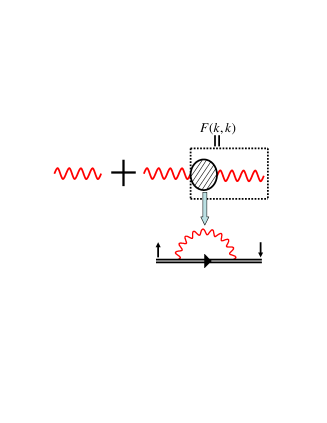
Figure 2: The Feynman diagram for the effective photon transmission through the CROW in a propagating mode. The photon propagator contains the free part (the bare photon propagator is denoted by a single wiggly line) and the second perturbation part (one wiggly line plus a box). The box includes the shade circle for the self energy of photon and the bare atom propagator( the double arrowed line).

We consider the weak-coupling case. On the right side of the equation of $\langle\langle\sigma_{k}^{-}|\sigma_{k}^{+}\rangle\rangle_{\omega}$ in Eq. (III) there are two terms, one is about the zero order of coupling constant $g$ and the other is about the second or higher order of $g$. Here we solve the equation of $\langle\langle\sigma_{k}^{-}|\sigma_{k}^{+}\rangle\rangle_{\omega}$ with the lowest order term of $g$:

$$\langle\langle\sigma_{k}^{-}|\sigma_{k}^{+}\rangle\rangle_{\omega}=-\frac{\langle\sigma^{z}\rangle}{f_{k}\left(\omega\right)}\text{.}$$ (20)

So we obtain the lowest order solution for

$$\langle\langle\hat{a}_{k}|\hat{a}_{k}^{{\dagger}}\rangle\rangle_{\omega}=\frac{\omega-\omega_{A}}{(\omega-\omega_{A})(\omega-\Omega_{k})+g^{2}\left\langle\sigma^{z}\right\rangle}\text{,}$$ (21)

and

$$\langle\langle\sigma_{k}^{-}|\sigma_{k}^{+}\rangle\rangle_{\omega}=\frac{-\langle\sigma^{z}\rangle(\omega-\Omega_{k})}{(\omega-\Omega_{k})(\omega-\omega_{A})+g^{2}\langle\sigma^{z}\rangle}\text{.}$$ (22)

There exist two poles $\omega=\omega_{k}^{(+)}$ and $\omega=\omega_{k}^{(-)}$:

$$\omega_{k}^{(\pm)}=\Omega_{D}\pm\epsilon_{k},$$ (23)

which are the dispersion relations. Here

$$\Omega_{D} =\frac{1}{2}(\omega_{A}+\Omega_{k})\text{,}$$ (24)

$$\epsilon_{k} =\frac{1}{2}\sqrt{(\Omega_{k}-\omega_{A})^{2}-4g^{2}\langle\sigma^{z}\rangle}\text{.}$$

We analyze the properties of the retarded Green functions of $\langle\langle\hat{a}_{k}|\hat{a}_{k}^{{\dagger}}\rangle\rangle_{\omega+i\varepsilon}$ and $\langle\langle\sigma_{k}^{-}|\sigma_{k}^{+}\rangle\rangle_{\omega+i\varepsilon}$ by decomposing them into two branches of wave, respectively. The propagating photons have the form as

$$\langle\langle\hat{a}_{k}|\hat{a}_{k}^{{\dagger}}\rangle\rangle_{\omega+i\varepsilon}=A_{k}G^{+}(k,\omega)+B_{k}G^{-}(k,\omega),$$ (25)

where the free Green functions are denoted by

$$G^{\pm}(k,\omega)=\frac{1}{\omega-\omega_{k}^{(\pm)}+i\varepsilon}\text{,}$$ (26)

and the atomic part has the form as

$$\langle\langle\sigma_{k}^{-}|\sigma_{k}^{+}\rangle\rangle_{\omega+i\epsilon}=-\langle\sigma^{z}\rangle[B_{k}G^{+}(k,\omega)+A_{k}G^{-}(k,\omega)]\text{,}$$

where

$$A_{k}=\frac{\omega_{k}^{(+)}-\omega_{A}}{\omega_{k}^{(+)}-\omega_{k}^{(-)}},B_{k}=\frac{\omega_{A}-\omega_{k}^{(-)}}{\omega_{k}^{(+)}-\omega_{k}^{(-)}}\text{,}$$ (27)

are the amplitudes of the two wave branches.

Transforming the Green functions above back to the real time representation, one can observe that the photons propagate with two frequencies $\omega_{k}^{(\pm)}$. If we regard the transmission of the localized photons as propagating wave, the two wave branches or two partial waves with $\omega_{k}^{(\pm)}$ have the amplitudes $A_{k}$ and $B_{k}$, respectively. For $\langle\langle\sigma_{k}^{-}|\sigma_{k}^{+}\rangle\rangle_{\omega}$ it has been observed that sup the total collection of the identical two-level atoms can be regarded as an ensemble of $N$ spins and thus its collective excitation can be described as spin waves, which are characterized by $\langle\langle\sigma_{k}^{-}|\sigma_{k}^{+}\rangle\rangle_{\omega}$. It is shown that the spin wave has two eigenfrequencies $\omega_{k}^{(\pm)}$, but with the twist amplitudes $B_{k}$ and $A_{k}$, respectively. (The detailed analysis is given in the appendix B.)

For the photons in the CROW from localized modes to propagating modes, we can now visualize the two wave branches as quasi-particle excitations by considering the existence of isolated poles of $\langle\langle\hat{a}_{k}|\hat{a}_{k}^{{\dagger}}\rangle\rangle_{\omega}$. Suppose that there are such poles $\omega_{k}^{(\pm)}\rightarrow\omega_{k}^{(\pm)}-i\gamma_{\pm}$ on the complex plane. They correspond to the life $1/\gamma_{\pm}$ of the quasi-particle excitations characterizing the two branches of propagating wave in the coupled cavity array. By phenomenologically adding imaginary parts $-i\gamma_{c}$ and $-i\gamma_{A}$ to the cavity eigenfrequency $\omega_{C}$ and the atomic level spacing $\omega_{A}$ respectively, $\gamma_{\pm}$ can be explicitly expressed obviously  in terms of $-i\gamma_{c}=$ $-i\kappa$ and $-i\gamma_{A}=-i\gamma$ (the details in the next section). This means that the decay of transporting photons is just induced by the cavity decay and the atom natural line width.

IV Coherent transmission of photons with slowed group velocity

From the dispersion relation (24), it can be observed that the population inversion $\langle\sigma^{z}\rangle$ can directly affect the basic features of coherent transmission of photons in the CROW. To enhance this influence, we put more doping atoms in a cavity. Suppose that every cavity is doped by $n$ identical atoms without interaction among themselves. Then the parts of the Hamiltonian in section II concerning atoms become

$$H_{A}=\sum_{\alpha=0}^{N-1}\frac{\omega_{A}}{2}S_{\alpha}^{z},H_{AC}=g\sum\limits_{\alpha=0}^{N-1}\hat{a}_{\alpha}S_{\alpha}^{+}+h.c.\text{,}$$

where we have introduced the collective spin $\mathbf{S}_{\alpha}=\sum_{l=1}^{n}\mathbf{\sigma}_{\alpha l}$. In this sense the above frequencies $\omega_{k}^{(\pm)}$ can be modified by replacing $\langle\sigma^{z}\rangle$ with

$$\langle S^{z}\rangle=\frac{1}{N}\sum_{\alpha=0}^{N-1}\sum_{l}^{n}\langle\sigma_{\alpha l}^{z}\rangle\text{.}$$ (28)

Obviously, the average of the total spin is bounded as $-n\leq\langle S^{z}\rangle\leq n$.

Before discussing the group velocity of photons, we investigate the change of bandwidth of this photonic-crystal-like system. Because the group velocity $v_{g}^{k}$ can be calculated according to $v_{g}^{k}=d\omega/dk$, which concerns the range of $\omega$, the change of bandwidth plays an important role. Without the doped atoms the spectrum of photons should have only one band, and the central line should be at $\omega_{C}$. However when atoms are doped, the spectrum splits into two bands with eigenfrequencies $\omega_{k}^{(\pm)}$. Then the central lines shift to $\Omega_{D}\pm\epsilon_{k=\pi/2\ell}$. Without population inversion, i.e.,$\langle S^{z}\rangle<0$, the two bands have the same width $W=\left|\omega_{k}^{(\pm)}|_{k=0}-\omega_{k}^{(\pm)}|_{k=\pi/2\ell}\right|<2J$, which is calculated as

$$W=|F_{\pm}(\left\langle S_{0}^{z}\right\rangle,0)-F_{\pm}(\left\langle S_{0}^{z}\right\rangle,\frac{\pi}{2\ell})|\text{,}$$ (29)

where

$$F_{\pm}(x,k)=\sqrt{\frac{1}{4}\left[\delta+J\cos(k\ell)\right]^{2}-g^{2}x}\text{,}$$ (30)

for $\delta=\omega_{C}-\omega_{A}$. This means that the bandwidth becomes narrower when cavities are coupled to more atoms.

Next we consider the group velocity of photon propagation

$$v_{g}^{(\pm)k}=J\ell\sin(k\ell)\left[1\pm\frac{\delta+2J\cos(k\ell)}{2F_{\pm}(\langle S^{z}\rangle,k)}\right]\text{,}$$ (31)

for various cases. At $k=\pi/2\ell$, the group velocities of $\omega_{\pi/2\ell}^{(\pm)}$ read

$$v_{g}^{(\pm)\pi/2\ell}=J\ell\left[1\pm\frac{\delta}{\varkappa}\right]\text{,}$$ (32)

and the amplitudes of the photon propagator can be calculated as

$$A_{\pi/2\ell}=\frac{\delta+\varkappa}{2\varkappa}\text{, }B_{\pi/2\ell}=\frac{-\delta+\varkappa}{2\varkappa}\text{,}$$ (33)

respectively, where $\varkappa=\sqrt{\delta^{2}-4g^{2}\langle S^{z}\rangle}$.

Figure 3: There are ten curves with $J\geq\delta\geq 0.1J$ in the fig(a)-(d), respectively. The group velocities of $v_{g}^{(+)}$, $v_{g}^{(-)}$ and the amplitudes $A_{k}$, $B_{k}$ are functions of coupling strength $g$ at $k=\pi/(2\ell)$. In the fig(a)-(d) the lattice constant $\ell=1$, $|<S^{z}>|=10$. In fig(a) and fig(b) the upper curves are for $\delta=J$, while in fig(c) and fig(d) the upper curves are for $\delta=0.1J$.

We now consider the case with most atoms in the ground state, i.e., $\langle S^{z}\rangle<0$.  When $\delta\gg 2g\sqrt{|\langle S^{z}\rangle|}$, the amplitude at the band center $A_{\pi/2\ell}\rightarrow 1$, $B_{\pi/2\ell}\rightarrow 0$, and then

$$\langle\langle\hat{a}_{\pi/2\ell}|\hat{a}_{\pi/2\ell}^{{\dagger}}\rangle\rangle_{\omega+i\varepsilon}\approx\frac{1}{\omega-\omega_{\pi/2\ell}^{(+)}+i\varepsilon}.$$ (34)

In other words, in this limit the photon modified by the atoms tends to have an eigenfrequency $\omega_{\pi/2\ell}^{(+)}$. Correspondingly the group velocity reaches its maximum $v_{g}^{(+)\pi/(2\ell)}\approx 2J\ell$, and the quasi-spin wave for the atomic excitations is characterized by the Green function

$$\langle\langle\sigma_{\pi/2\ell}^{-}|\sigma_{\pi/2\ell}^{+}\rangle\rangle_{\omega+i\varepsilon}\approx\frac{|\langle S^{z}\rangle|}{\omega-\omega_{\pi/2\ell}^{(-)}+i\varepsilon},$$ (35)

which has a distinct eigenfrequency $\omega_{\pi/2\ell}^{(-)}$. With $g\rightarrow 0$, $\omega_{\pi/2\ell}^{(+)}$ and $\omega_{\pi/2\ell}^{(-)}$ approach $\omega_{C}$ and $\omega_{A}$, respectively. On the contrary, when $\delta\ll-2g\sqrt{|\langle S^{z}\rangle|}$, we make a similar argument: as $A_{\pi/2\ell}\rightarrow 0$, $B_{\pi/2\ell}\rightarrow 1$, the photons and atomic spin wave propagate with eigenfrequencies $\ \omega_{\pi/2\ell}^{(-)}$ and $\omega_{\pi/2\ell}^{(+)}$, respectively. By letting $g\rightarrow 0$, $\omega_{\pi/2\ell}^{(+)}$ and $\omega_{\pi/2\ell}^{(-)}$ can be revived as $\omega_{A}$ and $\omega_{C}$, respectively. The group velocity of photons can also reach its maximum $v_{g}^{(-)\pi/2\ell}\approx 2J\ell$ (The detailed analysis is given in the appendix B). These observations are different from the results obtained in the simple cavity - cavity coupling system without atom doping in Ref.Fanprl04 .

Analyzing the features of eigenfrequencies $\omega_{k}^{(\pm)}$ for photon and atom parts in the case of weak coupling, we have observed that $\omega_{k}^{(\pm)}$ have different preferences to approach frequencies of pure photons or bare atoms. It is concluded from this observation that , if $\delta>0$, photons prefer $\omega_{k}^{(+)}$  while the atomic spin wave prefers $\omega_{k}^{(-)}$ ; if $\delta<0$, the conclusion is just on the contrary. We illustrate these analysis in Fig. 4.

Figure 4: In fig (a) and (b), $\omega_{\pi/(2\ell)}^{(+)}$(solid) and $\omega_{\pi/(2\ell)}^{(-)}$(dashed) are functions of coupling strength g and $|<S^{z}>|=10$. In fig (a) $\omega_{C}=2J$, $\omega_{A}=1.5J$ and $\delta=0.5J$, while in fig (b) $\omega_{C}=1.5J$, $\omega_{A}=2J$ and $\delta=-0.5J$.

Next we consider how a coherent pump induces population inversion to result in a laser-like output for the CROW. In the discussions above, we have considered an ideal case in which the quantum dissipation and dephasing due to the influence of the environment are neglected. Meanwhile, we have not concerned the role of $\langle S^{z}\rangle$, the average value of total atoms population. Here, we also assumed that $\langle S^{z}\rangle$ is not tunable . But for an open system, $\langle S^{z}\rangle$ becomes a time-dependent parameter. We can tune the population of atoms to change the properties of photon transmission. When the population inversion takes place, we expect that laser-like output emerges.

To see more details, let us consider a realistic case that the cavity damp has the same rate $\kappa$ and the atoms have the decay rate $\gamma$ due to spontaneous radiation. Then $\omega_{C}\rightarrow\omega_{C}-i\kappa$ and $\omega_{A}\rightarrow\omega_{A}-i\gamma$,  so the eigenfrequencies of photonic band become

$$\omega_{k}^{(\pm)}=\Omega_{D}-\frac{i\left(\gamma+\kappa\right)}{2}\pm\Omega_{\pm}\text{,}$$ (36)

where we define $\Lambda=\gamma-\kappa$ and

$$\Omega_{\pm}=\frac{1}{2}\sqrt{[\left(\Omega_{k}-\omega_{A}\right)-i\Lambda]^{2}-4g^{2}\langle S^{z}\rangle}\text{.}$$ (37)

For the sake of simplicity, we consider a special case that is $\Omega_{k}\approx\omega_{A}$, and $\gamma\gg\kappa$. Then the eigenfrequencies read

$$\omega_{k}^{(\pm)}=\Omega_{D}\pm\frac{i}{2}[f(\langle S^{z}\rangle)\gamma\mp\gamma\mp\kappa]\text{,}$$ (38)

where $f(x)=\sqrt{1+4xg^{2}/\gamma^{2}}$. If the imaginary part $\lambda$ of an eigenfrequency (e.g., $\omega_{k}^{(+)}$) is positive, the laser-like output will appear since a component $A_{k}/(\omega-\omega_{k}^{(+)})$ of $\langle\langle\hat{a}_{k}|\hat{a}_{k}^{{\dagger}}\rangle\rangle_{\omega}$ has a real time correspondence

$$A(t)=\int\frac{A_{k}d\omega}{\omega-\omega_{k}^{(+)}}\sim-i\theta(t)e^{-i\Omega_{D}t+\lambda t}\text{,}$$ (39)

where $A_{k}$ is a slowly varying amplitude in the $k$-space. Actually, when most of atoms stay at the ground state, i.e. $\langle S^{z}\rangle\leq 0$, it is impossible for $\omega_{k}^{(+)}$ and $\omega_{k}^{(-)}$ to have a positive imaginary part; when the population of most atoms inverts, i.e. $\langle S^{z}\rangle>0$, the imaginary part of $\omega_{k}^{(+)}$ may be positive.

Furthermore there is a threshold value of $\langle S^{z}\rangle$ to satisfy the condition $[f(\langle S^{z}\rangle)-1]\gamma>\kappa$. When $\langle S^{z}\rangle\ll\gamma^{2}/(4g^{2})$, we explicitly obtain the threshold value of $\left\langle S^{z}\right\rangle_{T}$ as

$$\langle S^{z}\rangle_{T}=\frac{\gamma\kappa}{2g^{2}}\text{.}$$ (40)

Above this threshold value, the eigenfrequency

$$\omega_{k}^{(+)}\sim\Omega_{D}+i(\frac{g^{2}}{\gamma}\langle S^{z}\rangle-\frac{\kappa}{2})$$ (41)

has a positive imaginary part, which results in a laser-like output in the CROW. It is very interesting that the $\langle S^{z}\rangle_{T}$ is very similar to the threshold value of population inversion in the generic laser theory. We also notice that, in weak-coupling limit, $\omega_{k}^{(-)}$ can not be a robust frequency of laser-like output since it damps fast with rate $\left[f\left(\langle S^{z}\rangle\right)+1\right]\gamma+\kappa$.

V Susceptibility analysis for light propagation in the doped CROW

The above analysis displays a possibility to implement a slow light propagation in the doped CROW, but the calculation of the group velocity from the dispersion relation shows that, only for certain wave vector $k,$ can the group velocity be reduced down. Thus for the propagation of a wave packet or a light pulse, we still need some details for the absorption and dispersion of light in the doped CROW. We use the dynamic algebraic method developed for the atomic ensemble based on quantum memory with EIT sunprl91 . The original method was proposed for the conventional EIT system, which consists of a vapor cell with three-level $\Lambda-$atoms near resonantly coupled to the controlling and quantized probe light. Our dynamic symmetry analysis is based on the hidden dynamic symmetry described by the semi-direct product of quasi-spin $SU(2)$ and the boson algebra of the excitations. This method allows us to build a dynamic equation describing the propagation of the probe light in this atomic ensemble with atomic collective excitations liyong .

Now we apply this algebraic method to calculate the susceptibility of light for the group velocity of photonic wave packet propagating along the doped CROW. Then we investigate how the susceptibility depends on the various control parameters.

We simplify our model by using the collective operators $b_{\alpha}=S_{\alpha}^{-}/\sqrt{n}$ and $b_{\alpha}^{{\dagger}}=S_{\alpha}^{+}/\sqrt{n}$, which represent the quasi-spin wave in the low-excitation limit that only few atoms populated in their excited state. In this case we can check that the spin wave is bosonic excitation since the boson commutation relation $[b_{\alpha},b_{\alpha^{\prime}}^{{\dagger}}]=\delta_{\alpha,\alpha^{\prime}}$ is satisfied in the low-excitation limit. Then the total Hamiltonian for the hybrid system with many-atom doping becomes

$$H =\omega_{C}\sum_{\alpha}a_{\alpha}^{{\dagger}}a_{\alpha}+J\sum_{\alpha}\left(a_{\alpha}^{{\dagger}}a_{\alpha+1}+a_{\alpha+1}^{{\dagger}}a_{\alpha}\right)$$

$$+\omega_{A}\sum_{\alpha}b_{\alpha}^{{\dagger}}b_{\alpha}+\sum_{\alpha}g\sqrt{n}\left(a_{\alpha}^{{\dagger}}b_{\alpha}+b_{\alpha}^{{\dagger}}a_{\alpha}\right).$$ (42)

Its $k$-space representation $H=\sum_{k}$ $H_{k}$ is a simple sum of the $k$-component

$$H_{k}=\Omega_{k}a_{k}^{{\dagger}}a_{k}+\omega_{A}b_{k}^{{\dagger}}b_{k}+g\sqrt{n}\left(a_{k}^{{\dagger}}b_{k}+h.c\right).$$ (43)

Here, we have used the Fourier transformation $b_{k}=\sum_{\alpha}\exp(ik\ell\alpha)b_{\alpha}/\sqrt{N}$.

For each mode $k$, we can write down the Heisenberg equations of operators $a_{k}$ and $b_{k}$.

$$i\partial_{t}a_{k} =-i\kappa a_{k}+\Omega_{k}a_{k}+g\sqrt{n}b_{k},$$

$$i\partial_{t}b_{k} =-i\gamma b_{k}+\omega_{A}b_{k}+g\sqrt{n}a_{k}.$$

Here, we have phenomenologically introduced the decay rates $\kappa$ and $\gamma$, and $\gamma\gg\kappa$. In the interaction picture, we adopt the time-dependent transformation,

$$a_{k}=\widetilde{a}_{k}e^{-i\Omega_{k}t},b_{k}=\widetilde{b}_{k}e^{-i\Omega_{k}t}$$ (44)

for $a_{k}$ and $b_{k}$ to remove the fast varying parts of the light field and the atomic collective excitations. Then the above equations of motion are reduced into

$$\partial_{t}\widetilde{a}_{k} =-\kappa\widetilde{a}_{k}-ig\sqrt{n}\widetilde{b}_{k},$$

$$\partial_{t}\widetilde{b}_{k} =-\gamma\widetilde{b}_{k}-i(\omega_{A}-\Omega_{k})b_{k}-ig\sqrt{n}\widetilde{a}_{k}.$$

In general the steady state solution of the equations above determines the susceptibility of photon transmission. It is noticed that the quantized light described by $a_{k}$ is the superposition of some localized modes $a_{j}$. On the contrary, the spatially distributed photon field is characterized by $a_{\alpha}=\sum_{k}\exp(-ik\ell\alpha)a_{k}/\sqrt{N},$which means the inhomogeneous polarization $\left\langle P_{\alpha}\right\rangle$ depends on the spatial position. Correspondingly, we have the $k$-space representation of the light field

$$E_{k}(t)=\sqrt{\frac{\omega_{C}}{2V\epsilon_{0}}}a_{k}e^{-i\Omega_{k}t}+h.c.$$ (45)

In comparison with the classical expression $E_{k}(t)=\epsilon_{k}\exp(-i\Omega_{k}t)+h.c.,$it is recognized that

$$\epsilon_{k}\sim\sqrt{\frac{\omega_{C}}{2V\epsilon_{0}}}a_{k}.$$

On the other hand the linear response of medium is described by the local polarization $\left\langle P_{k}\right\rangle=\left\langle p_{k}\right\rangle\exp(-i\Omega_{k}t)+h.c.$, where the average polarization

$$\left\langle p_{k}\right\rangle=\frac{\mu}{V}\sqrt{n}\langle\widetilde{b}_{k}\rangle$$ (46)

slowly varies  and determined by an average value of excitation operator $\widetilde{b}_{k}$; $\mu$ denotes the dipole moment of single atom, and $V$ is the effective mode volumebqoptics . It is related to the susceptibility $\chi_{k}$ of the $k$-space by

$$\chi_{k}=\frac{\left\langle p_{k}\right\rangle}{\left\langle\epsilon_{k}\right\rangle\epsilon_{0}}=\frac{\sqrt{n}\mu}{\left\langle\epsilon_{k}\right\rangle\epsilon_{0}V}\langle\widetilde{b}_{k}\rangle$$ (47)

since $\left\langle P_{k}\right\rangle=\chi_{k}E_{k}(t).$

To calculate the susceptibility in our case, we need the steady state solution satisfying $\partial_{t}\widetilde{b}_{k}=0$, or

$$\gamma\widetilde{b}_{k}+i(-\delta-2J\cos k\ell)\widetilde{b}_{k}+ig\sqrt{n}\widetilde{a}_{k}=0,$$

for $\gamma\gg\kappa$. Here, $\delta=\omega_{C}-\omega_{A}$ is the detuning between photons and atoms. In the steady state approach, we can take the expectation value for the above equation

$$ig\sqrt{n}\left\langle\widetilde{a}_{k}\right\rangle=-(\gamma-i\delta-2J\cos k\ell)\langle\widetilde{b}_{k}\rangle.$$

Since the dipole approximation $g=-\mu\sqrt{\omega_{C}/(2V\epsilon_{0})}$, the linear susceptibility

$$\chi_{k} \equiv\chi_{1k}+i\chi_{2k}$$

$$=\frac{2ig^{2}n}{\omega_{C}[\gamma-i(\delta+2J\cos k\ell)]}\text{.}$$

The real part

$$\chi_{1k}=\frac{-(\delta+2J\cos k\ell)2g^{2}n}{\omega_{C}[\gamma^{2}+(\delta+2J\cos k\ell)^{2}]}\text{,}$$ (48)

and the imaginary part

$$\chi_{2k}=\frac{2g^{2}n\gamma}{\omega_{C}[\gamma^{2}+(\delta+2J\cos k\ell)^{2}]}$$ (49)

are related to the dispersion and absorption of the light field in the CROW, respectively.

Figure 5: Real part $\chi_{1}$ (solid) and imaginary part $\chi_{2}$ (dashed) of the susceptibility $\chi$ vs the light detuning $\delta$ in normalized units of $\gamma$ according to: (a) $k=\pi/2\ell$ and $J=0.1$; (b) $k=\pi/\ell$ and $J=0.1$; (c) $k=0$ and $J=0.1$; (d) $k=0$ and $J=0.8$. The other parameters are given as: $\omega_{C}=1$ $g\sqrt{n}=1$.

Because the photons have the band structure, the properties of dispersion and absorption of photons vary with the the wave vector with momentum index $k$. While the real part $\chi_{1k}$ reaches its maximum at $\delta=-(\gamma+2J\cos k\ell)$, the imaginary part $\chi_{2k}$ reaches its maximum at $\delta=-2J\cos k\ell$ and thus the absorption is a considerable property of the system. Here, the photons with different wave vectors $k$ will have different character of absorption. Figure 5 (a)-(c) show the dependence of $\chi_{1k}$ and $\chi_{2k}$ on $k$. The maximums of the absorption for $k=\pi/2\ell$, $\pi/\ell$, $0$, appear at three different values of $\delta$. The reason for this phenomena is that the inter-cavity interaction with the coupling constant $J$ will shift the resonance point in general, but if $k=\pi/2\ell$, the coupling has no effect on for spectral structure. In view of our analysis, the absorption directly depends on the wave vector $k$. At the same time we can imagine that the character of absorption can influence the group velocity of photons. It is obvious to see that an unavoidable loss effect appears for the group velocity when the atom media absorbs light strongly. The dispersion relation of photons is described by $\Omega_{k}=\omega_{C}+2J\cos{k\ell}$ , from which we calculate the group velocity as

$$v_{g}^{k}=|\frac{d\Omega_{k}}{dk}|\propto 2J\ell.$$ (50)

But from Eq.(49) it can be seen that the media absorption characterized by $\chi_{2k}$, will be stronger when $2J\ell$ becomes smaller. In other words, the considerable absorption corresponds to a slow group velocity. Actually, since the effect of the group velocity is due to a spectrum structure of the wave vector $k$, only a small range of $k$ around the point corresponding to the minimum group velocity, avoided is the higher order dispersion. The the point of minimum group velocity and the point of maximum absorption are related and somewhat close. This fact means that there is some unavoidable loss.

VI Conclusion

We have studied the coherent transmission of photons with local modes along the CROW coupled to artificial two-level atoms. Under the weak-coupling limit, we use the stimulated Raman excitation to tune the level spacing of the effective two-level system so that the properties of photons in the CROW can be manipulated coherently. As the above results display, if we prepare the hybrid system as that $\omega_{C}\gg\omega_{A}$ or $\omega_{C}\ll\omega_{A},$ the group velocity of photons in the doped CROW will reach maximum under the two cases. Meanwhile the two eigenfrequencies of the hybrid system have preference that, while one tends to the frequency of photons, another tends to that of quasi-spin wave of the total atoms. By controlling the average population of the doping atoms in the CROW with decay, we predict that the laser-like output may occur. With such an exotic photonic band structure, the light with different $k$ has different properties of absorption.

In zhou about control of photon transmission in CROW by doping artificial atoms for various hybrid structures, we study the case of the resonate three-level doping atoms by making use of the quasi-spin wave theory based on a mean field method. This investigation will make a corporate effort for the coherent transmission of photons in an artificial structure, where both the EIT effect and the band-like structure are utilized simultaneously.

This work is supported by the NSFC with grant No.90403018, 10375038, 60433050, and NKBRPC with No.2004CB318000, and NFRPC with No. 2001CB309310 and 2005CB724508. One (LZ) of authors gratefully acknowledges the support of K. C. Wong Education Foundation, Hong Kong.

Appendix A Equations of motion for the two time Green function

In this appendix, we provide a detailed derivation of the approximately closed system of the equations for two-time Green functions as following text

$$\langle\langle\hat{a}_{k}|\hat{a}_{k}^{{\dagger}}\rangle\rangle_{\omega}\text{, }\langle\langle\sigma_{k^{\prime}}^{-}|\sigma_{k}^{+}\rangle\rangle_{\omega}\text{, }\langle\langle\sigma_{k}^{-}|\sigma_{k}^{+}\rangle\rangle_{\omega},$$

$$\langle\langle\hat{a}_{k}|\sigma_{k^{\prime}}^{+}\rangle\rangle_{\omega}\text{, and }\langle\langle\sigma_{k}^{-}|\hat{a}_{k^{\prime}}^{{\dagger}}\rangle\rangle_{\omega}.$$ (51)

From the commutation relation between $\hat{a}_{k}$ and $H$, the equation of $\langle\langle\hat{a}_{k}|\hat{a}_{k}^{{\dagger}}\rangle\rangle_{\omega}$ is obtained as

$$\omega\langle\langle\hat{a}_{k}|\hat{a}_{k}^{{\dagger}}\rangle\rangle_{\omega}=\langle[\hat{a}_{k},\hat{a}_{k}^{{\dagger}}]\rangle+\langle\langle[\hat{a}_{k},H]|\hat{a}_{k}^{{\dagger}}\rangle\rangle_{\omega},$$

or

$$(\omega-\Omega_{k})\langle\langle\hat{a}_{k}|\hat{a}_{k}^{{\dagger}}\rangle\rangle_{\omega}=1+g\langle\langle\sigma_{k}^{-}|\hat{a}_{k}^{{\dagger}}\rangle\rangle_{\omega}.$$ (52)

Since the above equation concerns the two-time Green function $\ \langle\langle\sigma_{k}^{-}|\hat{a}_{k}^{{\dagger}}\rangle\rangle_{\omega},$ we need its motion equation, but here, we first calculate the equation of$\langle\langle\sigma_{k^{\prime}}^{-}|\sigma_{k}^{+}\rangle\rangle_{\omega}$

$$\omega\langle\langle\sigma_{k^{\prime}}^{-}|\sigma_{k}^{+}\rangle\rangle_{\omega}=\langle[\sigma_{k^{\prime}}^{-},\sigma_{k}^{+}]\rangle+\langle\langle[\sigma_{k^{\prime}}^{-},H]|\sigma_{k}^{+}\rangle\rangle_{\omega}\text{,}$$

or

$$\omega\langle\langle\sigma_{k^{\prime}}^{-}|\sigma_{k}^{+}\rangle\rangle_{\omega} =\omega_{A}\langle\langle\sigma_{k^{\prime}}^{-}|\sigma_{k}^{+}\rangle\rangle_{\omega}$$ (53)

$$-\frac{g}{N}\sum_{k^{\prime\prime}\alpha}e^{-i(k^{\prime}-k^{\prime\prime})\ell\alpha}\langle\langle\sigma_{\alpha}^{z}\hat{a}_{k^{\prime\prime}}|\sigma_{k}^{+}\rangle\rangle_{\omega}$$

$$-\frac{1}{N}\sum_{\alpha=0}^{N-1}e^{-i(k^{\prime}-k)\ell\alpha}\langle\sigma_{\alpha}^{z}\rangle.$$

The mean field approximation  assumes that $\langle\sigma_{\alpha}^{z}\rangle$ can be factorized from $\langle\langle\sigma_{\alpha}^{z}\hat{a}_{k^{\prime\prime}}|\sigma_{k^{\prime}}^{+}\rangle\rangle_{\omega}$, i.e.,

$$\langle\langle\sigma_{\alpha}^{z}\hat{a}_{k^{\prime\prime}}|\sigma_{k^{\prime}}^{+}\rangle\rangle_{\omega}\approx\langle\sigma_{\alpha}^{z}\rangle\langle\langle\hat{a}_{k^{\prime\prime}}|\sigma_{k^{\prime}}^{+}\rangle\rangle_{\omega}$$ (54)

and then the above Green function hierarchy is cut off. Thus we get a system of Green function equations

$$\omega\langle\langle\sigma_{k^{\prime}}^{-}|\sigma_{k}^{+}\rangle\rangle_{\omega} \approx-\frac{g}{N}\sum_{k^{\prime\prime}\alpha}e^{-i(k^{\prime}-k^{\prime\prime})\ell\alpha}\langle\sigma_{\alpha}^{z}\rangle\langle\langle\hat{a}_{k^{\prime\prime}}|\sigma_{k}^{+}\rangle\rangle_{\omega}$$

$$\frac{-1}{N}\sum_{\alpha=0}^{N-1}e^{-i(k^{\prime}-k)\ell\alpha}\langle\sigma_{\alpha}^{z}\rangle+\omega_{A}\langle\langle\sigma_{k^{\prime}}^{-}|\sigma_{k}^{+}\rangle\rangle_{\omega},$$

or

$$\langle\langle\sigma_{k^{\prime}}^{-}|\sigma_{k}^{+}\rangle\rangle_{\omega} =-\frac{1}{N\left(\omega-\omega_{A}\right)}[\sum_{\alpha=0}^{N-1}e^{-i(k^{\prime}-k)\ell\alpha}\langle\sigma_{\alpha}^{z}\rangle$$ (55)

$$+g\sum_{k^{\prime\prime}\alpha}e^{-i(k^{\prime}-k^{\prime\prime})\ell\alpha}\langle\sigma_{\alpha}^{z}\rangle\langle\langle\hat{a}_{k^{\prime\prime}}|\sigma_{k}^{+}\rangle\rangle_{\omega}].$$

For $k=k^{\prime}$,  the  Green function $\left\langle\left\langle\sigma_{k}^{-}|\sigma_{k}^{+}\right\rangle\right\rangle_{\omega}$  satisfies

$$\left\langle\left\langle\sigma_{k}^{-}|\sigma_{k}^{+}\right\rangle\right\rangle_{\omega} =-\frac{1}{N\left(\omega-\omega_{A}\right)}[\sum_{\alpha=0}^{N-1}\langle\sigma_{\alpha}^{z}\rangle+$$

$$g\sum_{k^{\prime}\alpha}e^{-i(k-k^{\prime})\ell\alpha}\langle\sigma_{\alpha}^{z}\rangle\langle\langle\hat{a}_{k^{\prime}}|\sigma_{k}^{+}\rangle\rangle_{\omega}].$$ (56)

We notice that the equation of $\langle\langle\hat{a}_{k}|\sigma_{k^{\prime}}^{+}\rangle\rangle_{\omega}$ is given by

$$\omega\langle\langle\hat{a}_{k}|\sigma_{k^{\prime}}^{+}\rangle\rangle_{\omega}=\langle\langle[\hat{a}_{k},H]|\sigma_{k^{\prime}}^{+}\rangle\rangle_{\omega},$$

or

$$(\omega-\Omega_{k})\langle\langle\hat{a}_{k}|\sigma_{k^{\prime}}^{+}\rangle\rangle_{\omega}=g\langle\langle\sigma_{k}^{-}|\sigma_{k^{\prime}}^{+}\rangle\rangle_{\omega}.$$ (57)

In order to derive the equation about $\langle\langle\sigma_{k}^{-}|\hat{a}_{k^{\prime}}^{{\dagger}}\rangle\rangle_{\omega}$ , we use the second kind of motion equation (14b),

$$\omega\langle\langle\sigma_{k}^{-}|\hat{a}_{k^{\prime}}^{{\dagger}}\rangle\rangle_{\omega}=-\langle\langle\sigma_{k}^{-}|[\hat{a}_{k^{\prime}}^{{\dagger}},H]\rangle\rangle_{\omega},$$

or

$$(\omega-\Omega_{k^{\prime}})\langle\langle\sigma_{k}^{-}|\hat{a}_{k^{\prime}}^{{\dagger}}\rangle\rangle_{\omega}=g\langle\langle\sigma_{k}^{-}|\sigma_{k^{\prime}}^{+}\rangle\rangle_{\omega}.$$ (58)

By defining

$$\langle\sigma_{k^{\prime}k}^{z}\rangle =\frac{1}{N}\sum_{\alpha=0}^{N-1}e^{-i(k-k^{\prime})\ell\alpha}\langle\sigma_{\alpha}^{z}\rangle,$$

$$f_{k}\left(\omega\right) =(\omega-\omega_{A}+\frac{g^{2}\langle\sigma^{z}\rangle}{\omega-\Omega_{k}}),$$

the equations about $\langle\langle\sigma_{k}^{-}|\sigma_{k}^{+}\rangle\rangle_{\omega}$ and $\langle\langle\sigma_{k^{\prime}}^{-}|\sigma_{k}^{+}\rangle\rangle_{\omega}$ can be finally obtained as

$$f_{k}\left(\omega\right)\langle\langle\sigma_{k}^{-}|\sigma_{k}^{+}\rangle\rangle_{\omega}=-\langle\sigma^{z}\rangle-g^{2}\sum_{k^{\prime}\neq k}\langle\sigma_{k^{\prime}k}^{z}\rangle\frac{\langle\langle\sigma_{k^{\prime}}^{-}|\sigma_{k}^{+}\rangle\rangle_{\omega}}{\omega-\Omega_{k^{\prime}}},$$ (59)

$$f_{k^{\prime}}\left(\omega\right)\langle\langle\sigma_{k^{\prime}}^{-}|\sigma_{k}^{+}\rangle\rangle_{\omega} =-\langle\sigma_{k^{\prime}k}^{z}\rangle-\frac{g^{2}\langle\sigma_{kk^{\prime}}^{z}\rangle\langle\langle\sigma_{k}^{-}|\sigma_{k}^{+}\rangle\rangle_{\omega}}{(\omega-\Omega_{k})}$$ (60)

$$-g^{2}\sum_{k^{\prime\prime}\neq k,\neq k^{\prime}}\langle\sigma_{k^{\prime\prime}k^{\prime}}^{z}\rangle\frac{\langle\langle\sigma_{k^{\prime\prime}}^{-}|\sigma_{k}^{+}\rangle\rangle_{\omega}}{\omega-\Omega_{k^{\prime\prime}}}.$$

Appendix B Quasi-spin waves coupled to transferred photons

In this appendix we analyze the physical meaning represented by the Green functions for photons and atoms that we obtained in section III. First we explicitly rewrite the coefficients $A_{k}$ and $B_{k}$ in $\langle\langle\hat{a}_{k}|\hat{a}_{k}^{{\dagger}}\rangle\rangle_{\omega}$ and $\langle\langle\sigma_{k}^{-}|\sigma_{k}^{+}\rangle\rangle_{\omega}$ as

$$A_{k} =\frac{\omega_{k}^{(+)}-\omega_{A}}{\omega_{k}^{(+)}-\omega_{k}^{(-)}}$$ (61)

$$=\frac{\Delta_{k}+\sqrt{\Delta_{k}^{2}-4g^{2}\langle\sigma^{z}\rangle}}{2\sqrt{\Delta_{k}^{2}-4g^{2}\langle\sigma^{z}\rangle}}\text{,}$$

and

$$B_{k} =\frac{\omega_{A}-\omega_{k}^{(-)}}{\omega_{k}^{(+)}-\omega_{k}^{(-)}}$$ (62)

$$=\frac{-\Delta_{k}+\sqrt{\Delta_{k}^{2}-4g^{2}\langle\sigma^{z}\rangle}}{2\sqrt{\Delta_{k}^{2}-4g^{2}\langle\sigma^{z}\rangle}}\text{,}$$

where $\Delta_{k}=\Omega_{k}-\omega_{A}.$ Let $\omega_{C}-\omega_{A}=\delta.$ When $k=\pi/(2\ell),$ we obtain $G_{P}\equiv\langle\langle\hat{a}_{\pi/2\ell}|\hat{a}_{\pi/2\ell}^{{\dagger}}\rangle\rangle_{\omega}$ as

$$G_{P} =\frac{\delta+\sqrt{\delta^{2}-4g^{2}\langle\sigma^{z}\rangle}}{2\sqrt{\delta^{2}-4g^{2}\langle\sigma^{z}\rangle}}\frac{1}{\omega-\omega_{\pi/2\ell}^{(+)}}$$

$$+\frac{-\delta+\sqrt{\delta^{2}-4g^{2}\langle\sigma^{z}\rangle}}{2\sqrt{\delta^{2}-4g^{2}\langle\sigma^{z}\rangle}}\frac{1}{\omega-\omega_{\pi/2\ell}^{(-)}}.$$ (63)

From the above equation we can see that, when $\langle\sigma^{z}\rangle<0$, and $\delta\gg 2g\sqrt{|\langle\sigma^{z}\rangle|}$, the amplitudes at the band center

$$A_{\pi/2\ell}\longrightarrow 1\text{, }B_{\pi/2\ell}\rightarrow 0,$$

which means

$$\langle\langle\hat{a}_{\pi/2\ell}|\hat{a}_{\pi/2\ell}^{{\dagger}}\rangle\rangle_{\omega}\approx\frac{1}{\omega-\omega_{\pi/2\ell}^{(+)}}\text{,}$$ (64)

and the group velocity $v_{g}^{(\pi/2\ell)}\approx 2J\ell$. Meanwhile, if $g\longrightarrow 0$, the eigenfrequencies of photons and atoms correspondingly approximate to their original eigenfrequencies without coupling

$$\omega_{\pi/2\ell}^{(+)}\rightarrow\omega_{C}\text{, }\omega_{\pi/2\ell}^{(-)}\rightarrow\omega_{A}.$$ (65)

If detuning $\delta\ll-2g\sqrt{|\langle\sigma^{z}\rangle|}$, the values of amplitudes are in reverse

$$A_{\pi/2\ell}\longrightarrow 0\text{, }B_{\pi/2\ell}\rightarrow 1\text{.}$$ (66)

Thus the Green function of photon at the band center only has one wave

$$\langle\langle\hat{a}_{\pi/2\ell}|\hat{a}_{\pi/2\ell}^{{\dagger}}\rangle\rangle_{\omega}\approx\frac{1}{\omega-\omega_{\pi/2\ell}^{(-)}}\text{.}$$ (67)

It also can be obtained that $v_{g}^{(\pi/2\ell)}\approx 2J\ell$. Meanwhile, we can conclude that, when $g\longrightarrow 0$, the eigenfrequencies of photon and atom are recovered correspondingly by another way that

$$\omega_{\pi/2\ell}^{(-)}\rightarrow\omega_{C}\text{, }\omega_{\pi/2\ell}^{(+)}\rightarrow\omega_{A}.$$ (68)

Next we study the Green function of the doping atoms $G_{A}\equiv\langle\langle\sigma_{k}^{-}|\sigma_{k}^{+}\rangle\rangle_{\omega}$:

$$G_{A}=-\langle\sigma^{z}\rangle\left[\frac{A_{k}^{\prime}}{\omega-\omega_{k}^{(+)}}+\frac{B_{k}^{\prime}}{\omega-\omega_{k}^{(-)}}\right]$$ (69)

with amplitudes

$$A_{k}^{\prime}=\frac{\omega_{k}^{(+)}-\Omega_{k}}{\omega_{k}^{(+)}-\omega_{k}^{(-)}}=B_{k}\text{,}$$ (70)

and

$$B_{k}^{\prime}=\frac{\Omega_{k}-\omega_{k}^{(-)}}{\omega_{k}^{(+)}-\omega_{k}^{(-)}}=A_{k}\text{,}$$ (71)

which has the similar expression as those of photons. Thus we rewrite the atomic Green function as

$$G_{A}=-\langle\sigma^{z}\rangle[\frac{B_{k}}{\omega-\omega_{k}^{(+)}}+\frac{A_{k}}{\omega-\omega_{k}^{(-)}}]\text{.}$$ (72)

We also consider the situation at $k=\pi/(2\ell)$. First we assume $\langle\sigma^{z}\rangle<0$ and $\delta\gg 2g\sqrt{|\langle\sigma^{z}\rangle|}$, in this case, the value of the amplitudes approximate to one and zero respectively

$$A_{\pi/2\ell}\longrightarrow 1\text{, }B_{\pi/2\ell}\rightarrow 0\text{,}$$ (73)

and thus the Green function of the doping atoms becomes

$$\langle\langle\sigma_{\pi/2\ell}^{-}|\sigma_{\pi/2\ell}^{+}\rangle\rangle_{\omega}\approx|\langle\sigma^{z}\rangle|\frac{1}{\omega-\omega_{\pi/2\ell}^{(-)}}\text{.}$$ (74)

However, when $g\longrightarrow 0$,

$$\omega_{\pi/2\ell}^{(-)}\rightarrow\omega_{A}\text{, }\omega_{\pi/2\ell}^{(+)}\rightarrow\omega_{C}\text{.}$$ (75)

If $\langle\sigma^{z}\rangle<0$ and $\delta\ll-2g\sqrt{|\langle\sigma^{z}\rangle|}$, we have

$$A_{\pi/2\ell}\longrightarrow 0\text{, }B_{\pi/2\ell}\rightarrow 1\text{,}$$ (76)

and thus

$$\langle\langle\sigma_{\pi/2\ell}^{-}|\sigma_{\pi/2\ell}^{+}\rangle\rangle_{\omega}\approx|\langle\sigma_{0}^{z}\rangle|\frac{1}{\omega-\omega_{\pi/2\ell}^{(+)}}\text{.}$$

Meanwhile when $g\longrightarrow 0$, the eigen-frequencies

$$\omega_{\pi/2\ell}^{(+)}\rightarrow\omega_{A}\text{, }\omega_{\pi/2\ell}^{(-)}\rightarrow\omega_{C}\text{.}$$ (77)

Finally we conclude that if $\delta\gg 2g\sqrt{|\langle\sigma^{z}\rangle|}$, $\omega_{\pi/2\ell}^{(+)}$ is the eigenfrequency of photonic part while $\omega_{\pi/2\ell}^{(-)}$ is the eigenfrequency of atomic part; On the other hand if $\delta\ll-2g\sqrt{|\langle\sigma^{z}\rangle|}$, the $\omega_{\pi/2\ell}^{(-)}$ is the eigenfrequency of photonic part and $\omega_{\pi/2\ell}^{(+)}$ is the eigenfrequency of atomic part.

References

• (1) Q. F. Xu, S. Sandhu, M. L. Povinelli, J. Shakya, S. H. Fan, M. Lipson, Phys. Rev. Lett. 96, 123901 (2006).
• (2) R. W. Boyd, D. J. Gauthier, Nature 441, 701 (2006).
• (3) S. E. Harris, Phys. Today 50, 36 (1997).
• (4) M. D. Lukin, A. Imamoglu, Nature (London) 413, 273 (2001).
• (5) M. F. Yanik, S. H. Fan, Phys. Rev. Lett. 92, 083901 (2004).
• (6) D. G. Angelakis, M. F. Santos, S. Bose, quant-ph/0606159 (2006).
• (7) M. J. Hartmann, F. G. S. L. Brandao and M. B. Plenio, Nature Physics 2, 849 (2006)..
• (8) D. Greentree, C. Tahan, J. H. Cole, L. C. L. Hollenberg, Nature Physics 2, 856 (2006).
• (9) L. Zhou, Y. B. Gao, Z. Song, C. P. Sun, cond-mat/0608577, (2006).
• (10) C. P. Sun, Y. Li, X. F. Liu, Phys. Rev. Lett.  91, 147903 (2003).
• (11) Y. Li, C. P. Sun, Phys. Rev. A 69, 051802(R) (2004).
• (12) D. N. Zubarev, Soviet Phys Usp(English Trasl), 3, 320 (1960).
• (13) P. A. Wolff, Phys. Rev. 120, 814 (1960).
• (14) T. Izuyama, D. J. Kim, R. Kubo, J. Phys. Soc.(Japan) 18, 1025(1963).
• (15) M. O. Scully and M. S. Zubairy, Quantum Optics (Cambridge University Press, Cambridge, 1997).
• (16) Lan Zhou, Jing Lu, C. P. Sun, quant-ph/0611159, submitted to Phys. Rev. A.