Information-disturbance tradeoff for spin coherent state estimation

Abstract

We show how to quantify the optimal tradeoff between the amount of information retrieved by a quantum measurement in estimating an unknown spin coherent state and the disturbance on the state itself, and how to derive the corresponding minimum-disturbing measurement.

I Introduction

The tradeoff between information retrieved from a quantum measurement and the disturbance caused on the state of a quantum system is a fundamental concept of quantum mechanics and has received a lot of attention in the literature WH ; wod ; sc ; sten ; eng ; fuchs96.pra ; banaszek01.prl ; fuchs01.pra ; banaszek01.pra ; barnum02.xxx ; gmd ; ozw ; mista05.pra ; dema ; macca ; mf ; cv ; max ; paris ; buscmax . Such an issue is studied for both foundations and its enormous relevance in practice, in the realm of quantum key distribution and quantum cryptography key ; key2 .

Quantitative derivations of such a tradeoff have been obtained in the scenario of quantum state estimation hol ; qse . The optimal tradeoff has been derived in the following cases: in estimating a single copy of an unknown pure state banaszek01.prl , many copies of identically prepared pure qubits banaszek01.pra and qudits mf , a single copy of a pure state generated by independent phase-shifts mista05.pra , an unknown maximally entangled state max , an unknown coherent state cv and Gaussian state paris . Experimental realization of minimal-disturbing measurements has been also reported dema ; cv . Recently, the optimal tradeoff has been also derived for quantum state discrimination buscmax .

The problem is typically the following. One performs a measurement on a quantum state picked (randomly, or according to an assigned a priori distribution) from a known set, and evaluates the retrieved information along with the disturbance caused on the state. To quantify the tradeoff between information and disturbance, one can adopt two mean fidelities banaszek01.prl : the estimation fidelity $G$, which evaluates on average the best guess we can do of the original state on the basis of the measurement outcome, and the operation fidelity $F$, which measures the average resemblance of the state of the system after the measurement to the original one.

In this paper, we study the optimal tradeoff between estimation and operation fidelities when the state is a completely unknown spin coherent state.

Our results will be obtained by exploiting the group simmetry of the problem, which allows us to restrict our analysis on covariant measurement instruments. In fact, the property of covariance generally leads to a striking simplification of problems that may look intractable, and has been thoroughly used in the context of state and parameter estimation hol ; qse .

The derivation of the optimal tradeoff for spin coherent state estimation might find application in the problem of how to achieve a secure distribution of a private shared directional reference frame brs ; chiri . This task can be achieved by setting up a secure classical key using regular quantum key distribution, and then converting this into a private shared reference frame using the technique of Ref. chiri . However, it is conceivable that there may be some benefit to using a different, more direct protocol wherein one sends the systems by encoding the directional information over the public channel and monitors for eavesdropping upon them. If the signal states were $SU(2)$ coherent states, then the question of how much security can be achieved depends on the nature of the information gain—disturbance tradeoff.

The paper is organized as follows. In Sec. II we briefly review the concept of spin coherent states. In Sec. III we show that the tradeoff between estimation and disturbance can be studied without loss of generality by considering measurement instruments with a covariant symmetry with respect to the rotation group. In Sec. IV we show how to quantify the optimal information-disturbance tradeoff and to obtain the corresponding minimum-disturbing measurement. We close the paper in Sec. V with concluding remarks.

II Spin coherent states

In the infinite dimensional space of the harmonic oscillator states we can construct the creation and annihilation operators, $a^{\dagger},a$, obeying the boson commutation relation $[a,a^{\dagger}]=1$. The coherent states of such a system (harmonic oscillator coherent states) are eigenvectors of the annihilation operator $a|\alpha\rangle=\alpha|\alpha\rangle$ and can be obtained as displacements of the ground state $|0\rangle$:

$$|\alpha\rangle=D(\alpha)|0\rangle,\quad D(\alpha)=\exp(\alpha a^{\dagger}-\alpha^{*}a).$$ (1)

An important property of such coherent states is that they satisfy the lower bound on product of the dispersions of the position and momentum operators (or the quadrature operators) required by the Heisenberg uncertainty relation.

The concept of coherent states is not restricted to the infinite dimensional space. In a finite dimensional space one can introduce different kinds of coherent states perelomov . In this paper we shall concentrate on so called spin coherent states ($SU(2)$ coherent states), which we define below.

Let us consider the Hilbert space of spin states with total spin $j$, hence with dimension $d=2j+1$. By $|m\rangle$, $m=-j,-j+1,\dots,j-1,j$, we denote the basis consisting of the eigenvectors of $J_{z}$ operator. Spin coherent states are defined as rotations of the “ground” state $|-j\rangle$ by unitary operators from the irreducible $SU(2)$ representation in the $2j+1$ dimensional space:

$$|\theta,\phi\rangle=R_{\theta,\phi}|-j\rangle,\quad R_{\theta,\phi}=e^{i\theta(J_{x}\sin\phi-J_{y}\cos\phi)}.$$ (2)

The operator $R_{\theta,\phi}$ corresponds to a rotation by the angle $\theta$ around the axis $\vec{n}=[\sin\phi,-\cos\phi,0]$. For $j=1/2$ the dimension of the space is $d=2$ (qubit). In this case spin coherent states are actually all the pure states in the space (every pure state can be described by a direction on the Bloch sphere). In higher dimensions, however, spin coherent states constitute only a subset in the set of all states of a given Hilbert space, and, moreover, they approach harmonic oscillator coherent states when the dimension of the space tends to infinity spincoh .

One can decompose a spin coherent state $|\theta,\phi\rangle$ in the $J_{z}$-eigenvectors basis as follows perelomov

$$\langle m|\theta,\phi\rangle = \left(\begin{array}[]{c}2j\\ j+m\end{array}\right)^{1/2}$$

$$\times \left(-\sin\frac{\theta}{2}\right)^{j+m}\left(\cos\frac{\theta}{2}\right)^{j-m}\,e^{-i(j+m)\phi}\;,$$

A spin coherent state in a Hilbert space ${\cal H}$, with $\hbox{dim}({\cal H})=2j+1$ will be written as $|\psi_{g}\rangle=U_{g}|-j\rangle$, where $U_{g}$ is a unitary irreducible representation of the $SU(2)$ group in dimension $d$ nota1 . When performing averages on group parameters, for convenience we will take the normalized invariant Haar measure $dg$ over the group, i.e. $\int_{SU(2)}dg=1$, and we will also omit $SU(2)$ from the symbol of integral.

III Covariant instruments for the rotation group

A measurement process on a quantum state $\rho$ with outcomes $\{r\}$ is described by an instrument instr , namely a set of trace-decreasing completely positive (CP) maps $\{{\cal E}_{r}\}$. Each map is a superoperator that provides the state after the measurement

$$\rho_{r}=\frac{{\cal E}_{r}[\rho]}{\hbox{Tr}\{{\cal E}_{r}[\rho]\}}\;,$$ (6)

along with the probability of outcome

$$p_{r}=\hbox{Tr}\{{\cal E}_{r}[\rho]\}\;.$$ (7)

The set of positive operators $\{\Pi_{r}={\cal E}_{r}^{\vee}[I]\}$, where $\vee$ denotes the dual map satisfying $\hbox{Tr}\{{\cal E}^{\vee}[A]\,B\}=\hbox{Tr}\{A\,{\cal E}[B]\}$ for all $A$ and $B$, is known as positive operator-valued measure (POVM), and normalization requires the completeness relation $\sum_{r}{\cal E}^{\vee}_{r}=I$. This is equivalent to require that the map $\sum_{r}{\cal E}_{r}$ is trace-preserving. In the following we will denote a $SU(2)$ unitary map as ${\cal U}_{g}$, namely ${\cal U}_{g}[\rho]=U_{g}\rho U^{\dagger}_{g}$. Notice that ${\cal U}^{\vee}_{g}={\cal U}_{g^{-1}}$.

The operation fidelity $F$ evaluates on average how much the state after the measurement resembles the original one, in terms of the squared modulus of the scalar product. Hence, for a measurement of an unknown spin coherent state, one has

$$F=\int dg\sum_{r}\langle-j|{\cal U}_{g}^{\vee}\circ{\cal E}_{r}\circ{\cal U}_{g}[|-j\rangle\langle-j|]|-j\rangle\;,$$ (8)

By adopting a guess function $f$, for each measurement outcome $r$ one guesses a spin coherent states $|\psi_{f(r)}\rangle$, and the corresponding average estimation fidelity is given by

$$G = \int dg\sum_{r}\hbox{Tr}\{{\cal E}_{r}\circ{\cal U}_{g}[|-j\rangle\langle-j|]\}$$ (9)

$$\times \langle\psi_{f(r)}|{\cal U}_{g}[|-j\rangle\langle-j|]|\psi_{f(r)}\rangle\;.$$

We are interested in the optimal tradeoff between $F$ and $G$, and without loss of generality we can restrict our attention to covariant instruments, that satisfy

$${\cal U}^{\vee}_{g}\circ{\cal E}_{h}\circ{\cal U}_{g}={\cal E}_{g^{-1}h}\;.$$ (10)

In fact, for any instrument $\{{\cal E}_{r}\}$ and guess function $f$, it turns out that the covariant instrument

$$\widetilde{\cal E}_{h}=\sum_{r}{\cal U}_{h}\circ{\cal U}^{\vee}_{f(r)}\circ{\cal E}_{r}\circ{\cal U}_{f(r)}\circ{\cal U}^{\vee}_{h}\;$$ (11)

with continuous outcome $h\in SU(d)$, along with the guess $|\psi_{h}\rangle$, provides the same values of $F$ and $G$ as the original instrument $\{{\cal E}_{r}\}$. Moreover, for covariant instruments the optimal guess function automatically turns out to be the identity function.

It is useful now to consider the Jamiołkowski representation CJ ; max2 , that gives a one-to-one correspondence between a CP map ${\cal E}$ from ${\cal H}_{in}$ to ${\cal H}_{out}$ and a positive operator $R$ on ${\cal H}_{out}\otimes{\cal H}_{in}$ through the equations

$${\cal E}(\rho)=\hbox{Tr}_{in}[(I_{out}\otimes\rho^{\tau})R]\;,$$

$$R=({\cal E}\otimes I_{in})|\Phi\rangle\langle\Phi|\;,$$ (12)

where $|\Phi\rangle$ represents the (unnormalized) maximally entangled state of ${\cal H}_{in}\otimes{\cal H}_{in}$, and $\tau$ denotes the transposition on the fixed basis. When ${\cal E}$ is trace preserving, correspondingly one has $\hbox{Tr}_{out}[R]=I_{in}$. For covariant instruments ${\cal E}_{g}$ as in Eq. (10), the operator $R_{g}$ acts on ${\cal H}^{\otimes 2}$, and has the form

$$R_{g}=U_{g}\otimes U_{g}^{*}R_{0}U_{g}^{{\dagger}}\otimes U_{g}^{\tau}\;,$$ (13)

(where $*$ denotes complex conjugation) with $R_{0}\geq 0$, and the trace-preserving condition

$$\int dg\,\hbox{Tr}_{2}[R_{g}]=I\;.$$ (14)

From Eq. (13) and the identity (Schur’s lemma for irreducible group representations zelo )

$$\int dg\,U_{g}XU_{g}^{\dagger}=\frac{\hbox{Tr}[X]}{\hbox{Tr}[I]}I\;,$$ (15)

it follows that condition (14) is equivalent to

$$\hbox{Tr}[R_{0}]=2j+1\;.$$ (16)

IV Optimal information-disturbance tradeoff

For covariant instruments, the expressions of the fidelities $F$ and $G$ in Eqs. (8) and (9) can be rewritten as follows

$$F = \int dg\int dh\,\langle-j|{\cal U}_{g}^{\vee}\circ{\cal E}_{h}\circ{\cal U}_{g}[|-j\rangle\langle-j|]|-j\rangle$$ (17)

$$= \int dg\,\langle-j|{\cal E}_{g}[|-j\rangle\langle-j|]|-j\rangle\;,$$

$$G = \int dg\int dh\,\hbox{Tr}\{{\cal E}_{h}\circ{\cal U}_{g}[|-j\rangle\langle-j|]\}$$ (18)

$$\times \langle-j|{\cal U}^{\vee}_{h}\circ{\cal U}_{g}[|-j\rangle\langle-j|]|-j\rangle$$

$$= \int dg\,\hbox{Tr}\{{\cal E}_{g}[|-j\rangle\langle-j|]\}$$

$$\times \langle-j|{\cal U}_{g}[|-j\rangle\langle-j|]|-j\rangle\;,$$

where the covariance property (10) and the invariance of the Haar measure have been used. Moreover, using the isomorphism (12), we can write $F$ and $G$ as $F=\hbox{Tr}[R_{F}R_{0}]$ and $G=\hbox{Tr}[R_{G}R_{0}]$, where $R_{F}$ and $R_{G}$ are the following positive operators

$$R_{F} = \int dg\,U_{g}\otimes U_{g}^{*}\,|-j\rangle\langle-j|^{\otimes 2}\,U_{g}^{{\dagger}}\otimes U_{g}^{\tau}\;,$$ (19)

$$R_{G} = \int dg\,|\langle-j|U_{g}|-j\rangle|^{2}\,I\otimes(U_{g}^{*}\,|-j\rangle\langle-j|\,U_{g}^{\tau})$$ (20)

$$= I\otimes\hbox{Tr}_{1}[(|-j\rangle\langle-j|\otimes I)R_{F}]\;.$$

Using Schur’s lemma for reducible group representations zelo , one can evaluate the group integral in Eq. (19) from the identity

$$\int dg\,U_{g}\otimes U_{g}^{*}\,Y\,U_{g}^{{\dagger}}\otimes U_{g}^{\tau}$$

$$=\left(\int dg\,U_{g}\otimes U_{g}\,Y^{\theta}\,U_{g}^{{\dagger}}\otimes U_{g}^{\dagger}\right)^{\theta}$$

$$=\sum_{l=0}^{2j}\hbox{Tr}[Y^{\theta}P_{l}]\frac{P_{l}^{\theta}}{\hbox{Tr}{P_{l}}}\;,$$ (21)

where $\theta$ denotes the partial transpose on the second Hilbert space, and $P_{l}$ represents the projector on the subspace of ${\cal H}\otimes{\cal H}$ with total spin $l$. Then, one has

$$R_{F} = \frac{1}{4j+1}P_{2j}^{\theta}\;,$$ (22)

$$R_{G} = \frac{1}{4j+1}I\otimes\hbox{Tr}_{1}[(|-j\rangle\langle-j|\otimes I)P_{2j}]\;.$$ (23)

The optimal tradeoff between $F$ and $G$ can be found by looking for a positive operator $R_{0}$ that satisfies the trace-preserving condition (16) and maximizes a convex combination

$$pG+(1-p)F=\hbox{Tr}\{[pR_{G}+(1-p)R_{F}]R_{0}\}\;,$$ (24)

where $p\in[0,1]$ controls the tradeoff between the quality of the state estimation and the quality of the output replica of the state. Then, $R_{0}$ will provide a covariant instrument that achieves the optimal tradeoff. In fact, we are interested in maximizing the operation fidelity $F=\hbox{Tr}[R_{F}R_{0}]$, for a fixed value of the estimation fidelity $G=\hbox{Tr}[R_{G}R_{0}]$. This is equivalent to maximizing the convex combination (24). Indeed, suppose that for a given value of $p$, we find $R_{0}$ that maximizes (24). It is clear that for $G=\hbox{Tr}[R_{G}R_{0}]$ this map yields maximum possible $F$, because any higher $F$ would increase (24).

It turns out that for any $p$ the eigenvector corresponding to the maximum eigenvalue of $C(p)\equiv pR_{G}+(1-p)R_{F}$ is non degenerate and of the form nota2

$$|\chi\rangle=\sum_{n=-j}^{j}a_{n}|n\rangle|n\rangle\;,$$ (25)

with suitable positive $\{a_{n}\}$. Upon taking $R_{0}$ proportional to $|\chi\rangle\langle\chi|$ and satisfying (16), the corresponding covariant instrument will then be optimal.

Notice that one has

$$F_{min}\equiv\frac{2j+1}{4j+1}\leq F\leq 1\;,$$ (26)

$$G_{min}\equiv\frac{1}{2j+1}\leq G\leq\frac{2j+1}{4j+1}\equiv G_{max}\;,$$ (27)

where $G_{max}$ is the optimal estimation fidelity with corresponding operation fidelity $F_{min}$, and $G_{min}$ corresponds to the value of $G$ for a random guess of the unknown state. The values $G_{max}$, $F_{min}$ for the optimal estimation are obtained for $R_{0}=(2j+1)|-j\rangle\langle-j|^{\otimes 2}$, corresponding to a quantum measurement described by spin coherent state POVM, i.e.

$${\cal E}_{g}(\rho)=(2j+1)|\psi_{g}\rangle\langle\psi_{g}|\rho|\psi_{g}\rangle\langle\psi_{g}|\;.$$ (28)

On the other hand, the values $F=1$ and $G=G_{min}$ are obtained for $R_{0}=(2j+1)\sum_{n,m=-j}^{j}|n,n\rangle\langle m,m|$, which corresponds to the identity operation.

Once one recognizes that the eigenvector $|\chi\rangle$ is of the form as in Eq. (25), the optimization problem can be rewritten as

$$F=\frac{1}{4j+1}\,\max_{\{a_{n}\}}\sum_{n,m=-j}^{j}a_{n}a_{m}c^{2}_{n,m}$$ (29)

with the constraints

$$\frac{1}{4j+1}\sum_{n=-j}^{j}a_{n}^{2}c_{n,-j}^{2}=G\;,\qquad\sum_{n=-j}^{j}a_{n}^{2}=2j+1\;,$$ (30)

where $c_{n,m}$ denotes Clebsch-Gordan coefficients $c_{n,m}=\langle j,n;j,m|(2j),n+m\rangle$. Notice that from the property

$$\langle j_{1},n;j_{2},m|j,n+m\rangle=$$

$$(-1)^{j_{1}+j_{2}-j}\langle j_{2},m;j_{1},n|j,n+m\rangle$$ (31)

it follows that the matrix $(c_{n,m})$ is symmetric. One can solved numerically such a constrained maximization, thus obtaining the optimal tradeoff between the operation and the estimation fidelities, along with the corresponding optimal measurement instrument

$${\cal E}_{g}(\rho)=U_{g}\xi U_{g}^{\dagger}\,\rho U_{g}\xi U_{g}^{\dagger}\;,$$ (32)

with $\xi=\sum_{n=-j}^{j}a_{n}|n\rangle\langle n|$.

For example, in the histogram of Fig. 1, we plot the optimal coefficients $\{a_{n}\}$ for the minimum-disturbing measurement of a spin coherent state with $j=2$ and fixed estimation fidelity $G=1/2$, for which the maximum value of the operation fidelity $F\simeq 0.795$ is achieved.

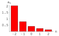
Figure 1: Optimal coefficients $\{a_{n}\}$ that provide through Eq. (32) the minimum-disturbing measurement for the estimation of a spin coherent state with $j=2$ and fixed estimation fidelity $G=1/2$, for which the maximum value of the operation fidelity $F\simeq 0.795$ is achieved.

We can introduce two normalized quantities that can be interpreted as the average information $I$ retrieved from the quantum measurement and the average disturbance $D$ affecting the original quantum state as follows:

$$I=\frac{G-G_{min}}{G_{max}-G_{min}}\;,$$ (33)

and

$$D=\frac{1-F}{1-F_{min}}\;.$$ (34)

Clearly, one has $0\leq I\leq 1$, and $0\leq D\leq 1$.

Figure 2: Optimal information-disturbance tradeoff in estimating an unknown spin coherent state for $j=1$ (solid line), and a harmonic oscillator coherent state (dotted line), where $I$ and $D$ are defined through Eqs. (33) and (34) in terms of the estimation and operation fidelities $G$ and $F$, respectively. For given value of the retrieved information $I$, the curve $D(I)$ are a lower bound for the disturbance of any measurement instrument.

In Fig. 2 (solid line) we plot the optimal information-disturbance tradeoff, for $j=1$. The curve $D(I)$ represents a lower bound for the disturbance of any measurement instrument that gathers information I. The bound is achieved by a covariant instrument as in Eq. (32). The optimal tradeoff $D(I)$ depends very slighly on the value of the spin $j$. In fact, it is known that for $j\to\infty$, spin coherent states approach the standard coherent states of harmonic oscillator spincoh . From Eq. (5) of Ref. cv , for harmonic oscillator coherent states one can obtain the following expression for the optimal information-disturbance tradeoff

$$D(I)=1-\sqrt{\frac{2(1-I)}{2-I}}\,,$$ (35)

which has been plotted in dotted line in Fig. 2.

We can consider the quantity $\hbox{Tr}[\xi]=\sum_{n=-j}^{j}a_{n}$ as a global quantity that characterizes the measurement instrument of Eq. (32) achieving the optimal tradeoff. In fact, using Jensen’s inequality, one has

$$\sqrt{2j+1}\leq\hbox{Tr}[\xi]\leq 2j+1\;,$$ (36)

where the lower and upper bound correspond to the optimal estimation map (28) and the identity map (with no information neither disturbance), respectively. Notice that $\hbox{Tr}[\xi]$ is related to the projection of the optimal bipartite vector $R_{0}$ on the maximally entangled vector $|\Phi\rangle=\sum_{n=-j}^{j}|n\rangle|n\rangle$ by the relation $\hbox{Tr}[\xi]=\sqrt{\langle\Phi|R_{0}|\Phi\rangle}$. In Fig. 3, we plot the value of $\hbox{Tr}[\xi]$ for the minimum-disturbing measurement versus the information, for spin $j=1$.

Figure 3: The quantity $\hbox{Tr}[\xi]$ for the measurement instrument of Eq. (32) that achieves the optimal information-disturbance tradeoff versus the information $I$, for spin $j=1$.

V Conclusions

In conclusion, we have shown how to derive the optimal tradeoff between the quality of estimation of an unknown spin coherent state and the degree the initial state has to be changed by this operation. The optimal tradeoff can be achieved by a covariant measurement instrument as in Eq. (32). By suitable normalization of the estimation and operation fidelities, the optimal tradeoff is shown to be almost independent of the value of the spin $j$.

In the case of estimation of an unknown pure state banaszek01.prl or maximally entangled state max , the minimum-disturbing measurement is simply the “coherent superposition” of the measurement instrument for optimal estimation and the identity map, namely the Kraus operators achieving the optimal information-disturbance tradeoff are just the sum of those corresponding to maximum information extraction and minimum disturbance. For spin coherent state, the solution is more complex. This is due to the fact that the derivation of the tradeoff in a covariant estimation problem involves the evaluation of group integrals as in $R_{F}$ and $R_{G}$. Generally, such integrals give a sum of $N$ operators, where $N$ is the number of invariant subspaces of the representation $U_{g}\otimes U_{g}^{*}$, and the optimal Kraus operators are the sum of $N$ corresponding terms. For pure states or maximally entangled states, $U_{g}\in SU(d)$ in dimension $d$, and $N=2$ (the symmetric and antisymmetric subspaces). For spin coherent states, $U_{g}$ is a unitary irreducible representation of $SU(2)$ in dimension $2j+1$, and the invariant subspaces of $U_{g}\otimes U_{g}^{*}$ are $N=2j+1$. Correspondingly, the Kraus operators of the minimum-disturbing measurement are given by a sum of $2j+1$ operators.

References

- (1) W. Heisenberg, Zeitsch. Phys. 43, 172 (1927).
- (2) K. Wódkiewicz, Phys. Lett. A 124, 207 (1987).
- (3) M. O. Scully, B.-G. Englert, and H. Walther, Nature 351, 111 (1991).
- (4) S. Stenholm, Ann. Phys. 218, 233 (1992).
- (5) B.-G. Englert, Phys. Rev. Lett. 77, 2154 (1996).
- (6) C. A. Fuchs and A. Peres, Phys. Rev. A 53, 2038 (1996).
- (7) K. Banaszek, Phys. Rev. Lett. 86, 1366 (2001).
- (8) C. A. Fuchs and K. Jacobs, Phys. Rev. A 63, 062305 (2001).
- (9) K. Banaszek and I. Devetak, Phys. Rev. A 64, 052307 (2001).
- (10) H. Barnum, quant-ph/0205155.
- (11) G. M. D’Ariano, Fortschr. Phys. 51, 318 (2003).
- (12) M. Ozawa, Ann. Phys. 311, 350 (2004).
- (13) L. Mišta Jr., J. Fiurášek, and R. Filip, Phys. Rev. A 72, 012311 (2005).
- (14) L. Mišta Jr. and J. Fiurášek, Phys. Rev. A 74, 022316 (2005).
- (15) F. Sciarrino, M. Ricci, F. De Martini, R. Filip, and L. Mišta Jr., Phys. Rev. Lett. 96, 020408 (2006).
- (16) L. Maccone, Phys. Rev. A 73, 042307 (2006).
- (17) U. L. Andersen, M. Sabuncu, R. Filip, and G. Leuchs, Phys. Rev. Lett. 96, 020409 (2006).
- (18) M. F. Sacchi, Phys. Rev. Lett. 96, 220502 (2006).
- (19) M. G. Genoni and M. G. A. Paris, Phys. Rev. A 74, 012301 (2006).
- (20) F. Buscemi and M. F. Sacchi, Phys. Rev. A 74, 052320 (2006).
- (21) C. H. Bennett and G. Brassard, in Proceedings of the IEEE International Conference on Computers, Systems, and Signal Processing, Bangalore, India (IEEE, New York, 1984), p. 175; C. H. Bennett, Phys. Rev. Lett. 68, 3121 (1992); N. Gisin, G. Ribordy, W. Tittel, and H. Zbinden, Rev. Mod. Phys. 74, 145 (2002).
- (22) A. K. Ekert, Phys. Rev. Lett. 67, 661 (1991); Nature 358, 14 (1992).
- (23) A. S. Holevo, Probabilistic and Statistical Aspects of Quantum Theory (North Holland, Amsterdam, 1982).
- (24) S. Massar and S. Popescu, Phys. Rev. Lett. 74, 1259 (1995); R. Derka, V. Buzek, and A. K. Ekert, Phys. Rev. Lett. 80, 1571 (1998); J. I. Latorre, P. Pascual, and R. Tarrach, Phys. Rev. Lett. 81, 1351 (1998); G. Vidal, J. I. Latorre, P. Pascual, and R. Tarrach, Phys. Rev. A 60, 126 (1999); A. Acín, J. I. Latorre, and P. Pascual, Phys. Rev. A 61, 022113 (2000); G. Chiribella, G. M. D’Ariano, P. Perinotti, and M. F. Sacchi, Phys. Rev. A 70, 062105 (2004); G. Chiribella, G. M. D’Ariano, P. Perinotti, and M. F. Sacchi, Phys. Rev. Lett. 93, 180503 (2004); G. Chiribella, G. M. D’Ariano, and M. F. Sacchi, Phys. Rev. A 72, 042338 (2005).
- (25) S. D. Bartlett, T. Rudolph, and R. W. Spekkens, Phys. Rev. A 70, 032307 (2004).
- (26) G. Chiribella, L. Maccone, and P. Perinotti, e-print quant-ph/0608042.
- (27) A. Perelomov, Generalized Coherent States and Their Applications (Springer-Verlag, Berlin, 1986).
- (28) F. T. Arecchi, E. Courtens, R. Gilmore, and H. Thomas, Phys. Rev. A 6, 2211 (1972).
- (29) More precisely, a spin coherent state corresponds to a point of the two-dimensional sphere , where the quotient group takes into account the stability group corresponding to the rotations around the -axis, which leave the state invariant, a part from irrelevant phase factor.
- (30) E. B. Davies and J. T Lewis, Commun. Math. Phys. 17, 239 (1970); K. Kraus, States, Effects, and Operations (Springer-Verlag, Berlin, 1983); M. Ozawa, J. Math. Phys. 25, 79 (1984).
- (31) A. Jamiołkowski, Rep. Math. Phys. 3, 275 (1972).
- (32) M. F. Sacchi, Phys. Rev. A 63, 054104 (2001).
- (33) D. P. Zhelobenko, Compact Lie Groups and Their Representations (American Mathematical Society, Providence, RI, 1973).
- (34) Such a result can be checked, for example, by means of the power method pm .
- (35) E. Isaacson and H. B Keller, Analysis of numerical methods (Dover, N. Y., 1994).