Quantum-limited force measurement with an optomechanical device

Abstract

We study the detection of weak coherent forces by means of an optomechanical device formed by a highly reflecting isolated mirror shined by an intense and highly monochromatic laser field. Radiation pressure excites a vibrational mode of the mirror, inducing sidebands of the incident field, which are then measured by heterodyne detection. We determine the sensitivity of such a scheme and show that the use of an entangled input state of the two sideband modes improves the detection, even in the presence of damping and noise acting on the mechanical mode.

I Introduction

Optomechanical systems play a crucial role in a variety of precision measurement like gravitational wave detection grav and atomic force microscopes afm . These systems are based on the interaction between a movable mirror, the probe experiencing the force to be measured, and a radiation field, the meter reading out the mirror’s position, which is due to the radiation pressure force acting on the mirror. The mechanical force exerts a momentum and position shift of a given vibrational mode of the mirror, which in turn induces a phase shift of the reflected optical field. A phase-sensitive measurement of the reflected light provides therefore a measurement of the force.

These optomechanical force detectors have a sensitivity which is limited by the thermal noise acting on the mirror mechanical degrees freedom, as well as by the more fundamental, unavoidable, quantum noise associated with the quantum nature of light, i.e., the phase fluctuations of the incident laser beam (shot noise) and the radiation pressure noise, inducing unwanted fluctuations of the mirror position. A compromise between these noises leads to the so-called standard quantum limit (SQL) for the sensitivity of the measurement caves ; BK92 . Analogous fundamental limitations affect also other similar detection devices, such as nano- and micro-electromechanical systems, which are also extensively studied for the realization of ultra-sensitive detection devices nems such as force detection on the atto-Newton level RUK and mass detection on the zepto-gram level SER .

Many proposals for the detection of weak forces involves high-finesse optical cavities with a movable mirror, in which the phase sensitivity is proportional to the cavity finesse qlock . However, recently Ref. FMT04 has proposed a new optomechanical detection scheme involving a single highly reflecting mirror, shined by an intense highly monochromatic laser pulse. A vibrational mode of the mirror induces two sidebands of the incident field, the Stokes and anti-Stokes sideband. This effect was recently observed in a micro-mechanical resonator as a consequence of the radiation pressure force acting on it VAHA . Under appropriate conditions on the duration of the laser pulse, the two sideband modes show significant two-mode squeezing, i.e., they are strongly entangled PM+03 . In particular the difference between the two amplitude quadratures and the sum of the phase quadratures of the sideband modes can be highly squeezed pirjmo , and this reduced noise properties are used in Ref. FMT04 to achieve high-sensitive detection of a force acting on the mirror. However Ref. FMT04 considered only partially the effect of the thermal environment of the mechanical mode. In fact, Ref. FMT04 considered the limiting case of a laser pulse duration much shorter than the mechanical relaxation time and neglected all the dynamical effects of damping and thermal noise. Here we drop this assumption and we take into account the effects of the thermal environment acting on the mechanical mode, by adopting a quantum Langevin equation treatment Gard91 . We shall see that, as expected, damping and thermal noise have a detrimental effect on the force detection sensitivity, but that one can still go below the SQL at achievable values of mechanical damping and temperatures, provided that the two sideband modes are appropriately entangled at the input.

The outline of the paper is as follows. In Sec. II we illustrate the model describing the force detection scheme, while in Sec. III we define and evaluate the minimum detectable force. In Sec. IV we consider experimentally achievable parameters and compare the performance of the scheme with the SQL for the detection of a force BK92 , while Sec. V is for concluding remarks.

II The Model

We consider the system schematically depicted in Fig. 1. It consists of a perfectly reflecting mirror shined by a pulsed quasi-monochromatic laser at main frequency $\omega_{0}$, linearly polarized in the mirror surface and focused in such a way as to excite the Gaussian acoustic modes of the mirror, in which only a small portion of the mirror around its center vibrates.

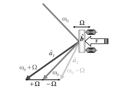
Figure 1: Schematics of the opto-mechanical device to detect a force F. A vibrational mode of the mirror (probe) related to the ladder operator $\hat{b}$ and oscillating at angular frequency $\Omega$ is excited by the radiation pressure of the incident laser field (angular frequency $\omega_{0}$). Light is scattered into the two first sideband modes, the anti-Stokes mode at $\omega_{0}+\Omega$ (operator $\hat{a}_{1}$) and the Stokes mode at $\omega_{0}-\Omega$ (operator $\hat{a}_{2}$). The force F to be detected acts on the mirror along the horizontal direction.

These modes describe elastic deformations of the mirror along the direction orthogonal to the surface, and are characterized by a small waist $w$, a large mechanical quality factor $Q$ and a small effective mass $M$. The motion of the mirror is actually determined by the excitation of several modes with different resonant frequencies. However, a single frequency mode can be considered when a bandpass filter in the detection scheme is used Pinard and mode-mode coupling is negligible. Therefore we will consider a single mechanical mode of the mirror only, which can be modeled as an harmonic oscillator with mass equal to the effective mass $M$ and angular frequency $\Omega$,

$$H_{0}=\frac{P_{b}^{2}}{2M}+\frac{1}{2}M\Omega^{2}X_{b}^{2},$$ (1)

where $X_{b}$ and $P_{b}$ are position and momentum operators of the chosen Gaussian vibrational mode, satisfying the commutation rule $[X_{b},P_{b}]=i\hbar$.

As demonstrated in Ref. PM+03 , in the case of an intense classical incident laser field and neglecting fast terms oscillating at $\pm\Omega$, the interaction between the chosen vibrational mode and the continuum of electromagnetic modes can be written, in the interaction picture (IP) with respect to the free Hamiltonian of the system, as a simple bilinear Hamiltonian involving the vibrational mode and the two first optical sideband modes

$$\tilde{H}_{int}=i\hbar\chi\left(\tilde{a}_{1}^{+}\tilde{b}^{+}-\tilde{a}_{1}\tilde{b}\right)+i\hbar\theta\left(\tilde{a}_{2}^{+}\tilde{b}-\tilde{a}_{2}\tilde{b}^{+}\right),$$ (2)

where $b$ is the annihilation operator of the vibrational mode given by $b=\left(iP_{b}+M\Omega X_{b}\right)/\sqrt{2\hbar M\Omega}$, $a_{k}$ are the annihilation operators of the optical sidebands Stokes ($k=1$, angular frequency $\omega_{0}-\Omega$) and anti-Stokes ($k=2$, angular frequency $\omega_{0}+\Omega$) modes, and the tilded operators are those in the IP. The coupling constants in Eq. (2) are given by PM+03

$$\chi = \cos\phi_{0}\sqrt{\frac{{\wp}\Delta\nu_{det}^{2}(\omega_{0}-\Omega)}{2M\Omega c^{2}\Delta\nu_{mode}}},$$ (3)

$$\theta = \chi\sqrt{\frac{\omega_{0}+\Omega}{\omega_{0}-\Omega}},$$ (4)

where $\phi_{0}$ is the angle of incidence of the driving beam, $\wp$ is the power of the incident beam and $\Delta\nu_{mode}$ is its bandwidth, while $\Delta\nu_{det}$ is the detection bandwidth.

II.1 Including damping and thermal noise on the vibrational motion

The performance of the three-mode optomechanical system described by Eq. (2) as a detector of a weak classical force acting on the mirror has been studied in Ref. FMT04 . In this latter paper, dynamical effects of the thermal environment of the mirror were ignored, because the dynamics have been studied only in the limit of interaction times much shorter than the mechanical damping time. Here we consider the more realistic situation of non-negligible mechanical damping, which, due to the fluctuation-dissipation theorem, implies also considering the effect of thermal noise on the mirror vibrational mode. These effects are described in terms of a quantum Langevin equation (QLE) for the vibrational mode which, in the first Markov approximation, can be written as Gard91

$$\overset{\cdot}{Y}=\frac{i}{\hbar}\left[H_{0}+H_{int},Y\right]-\frac{i}{2\hbar}\left\{\left[X_{b},Y\right],\xi(t)-\eta\overset{\cdot}{X}_{b}\right\},$$ (5)

where the brackets $\{,\}$ represent the anti-commutator, $Y$ is a generic Heisenberg-picture operator, $\eta$ is the damping coefficient of the mirror and $\xi(t)$ is the stochastic noise force, with correlation function Gard91 ; GV01

$$\left\langle\xi(t)\xi(t^{\prime})\right\rangle=\hbar\eta\int_{-\infty}^{\infty}\frac{d\omega}{2\pi}e^{-i\omega(t-t^{\prime})}\omega\left[\coth\left(\frac{\hbar\omega}{2k_{B}T}\right)+1\right],$$ (6)

where $k_{B}$ is the Boltzmann constant and $T$ is the equilibrium temperature. Applying Eq. (5) for the mirror position and momentum operators, we get

$$\overset{\cdot}{X_{b}} =\frac{P_{b}}{M}+i[H_{int},X_{b}]$$

$$\overset{\cdot}{P_{b}} =-M\Omega^{2}X_{b}+i[H_{int},P_{b}]-\overset{\cdot}{\eta X_{b}}+\xi(t),$$

implying the following evolution equation for $b$:

$$\overset{\cdot}{b} = -i\Omega b+\frac{i}{\hbar}[H_{int},b]-\frac{\eta}{2M}\left(b-b^{+}\right)$$ (7)

$$+i\sqrt{\frac{1}{2M\hbar\Omega}}\xi(t)+\frac{\eta}{2\hbar M\Omega}[H_{int},b+b^{+}].$$

If we now move to the IP we get

$$\overset{\cdot}{\tilde{b}} =\frac{i}{\hbar}[\tilde{H}_{int},\tilde{b}]-\frac{\eta}{2M}\left(\tilde{b}-\tilde{b}^{+}\right)$$

$$+i\sqrt{\frac{1}{2M\hbar\Omega}}e^{i\Omega t}\xi(t)+\frac{\eta}{2M\hbar\Omega}[\tilde{H}_{int},\tilde{b}+\tilde{b}^{+}].$$ (8)

By virtue of Eq. (2) we have:

$$\frac{\tilde{H}_{int}}{\hbar\Omega}\simeq\frac{\chi}{\Omega}\simeq\frac{\theta}{\Omega}.$$

This ratio is usually very low when realistic values are taken into account ($\chi\simeq\theta\sim 10^{5}$ s^-1, $\Omega\sim 10^{8}$ s^-1) PM+03 . Then the last term of Eq. (8) is much smaller than the second term, and can be neglected. Moreover, the term $\tilde{b}^{+}$ is counter-rotating and since we have already neglected fast oscillating terms at the frequency $\Omega$, we have to neglect it in Eq. (8) for consistency. In this way we arrive at the final quantum Langevin equation for the vibrational mode in the IP

$$\overset{\cdot}{\tilde{b}}=\frac{i}{\hbar}\left[\tilde{H}_{int},\tilde{b}\right]-2\gamma\tilde{b}+2\sqrt{\gamma}\tilde{b}_{in},$$ (9)

where we have defined the damping rate $\gamma$ and the scaled noise $\tilde{b}_{in}(t)$ as

$$\gamma = \frac{\eta}{4M},$$ (10)

$$\tilde{b}_{in}(t) = i\frac{e^{i\Omega t}\xi(t)}{\sqrt{2\eta\hbar\Omega}}.$$ (11)

In the limit of large $\Omega$ we are considering, the correlation functions of this latter noise term becomes simple. In fact, using Eq. (6) and the fact that the factor $e^{i\Omega t}$ is rapidly oscillating within the timescales of interest, it is possible to derive the following correlation properties of $\tilde{b}_{in}(t)$ Gard91-bis ,

$$\langle\tilde{b}_{in}(t)\tilde{b}_{in}(t^{\prime})\rangle = 0,$$ (12a)

$$\langle\tilde{b}_{in}(t)\tilde{b}_{in}^{\dagger}(t^{\prime})\rangle = (1+\overline{n})\delta(t-t^{\prime}),$$ (12b)

$$\langle\tilde{b}_{in}^{\dagger}(t)\tilde{b}_{in}(t^{\prime})\rangle = \overline{n}\delta(t-t^{\prime}),$$ (12c)

where $\overline{n}=1/(e^{\hbar\Omega/k_{B}T}-1)$ is the mean thermal vibrational number at the equilibrium temperature $T$. To state it in an equivalent way, in the limit of large $\Omega$, the properties of the Brownian noise acting on the vibrational mode become similar to those of the input noise of optical systems.

II.2 Exact solution of the dynamics

The Stokes and anti-Stokes modes are not directly sensitive to the damping and noise acting on the mirror. Moreover they do not undergo additional loss mechanisms since they are traveling waves. Therefore, the Heisenberg-Langevin equations describing the dynamics of the whole system, in the presence of an additional constant force acting on the mirror with dimensionless strength $f$, are

$$\dot{\tilde{a}}_{1} = \chi\tilde{b}^{\dagger}$$ (13a)

$$\dot{\tilde{b}} = \chi\tilde{a}_{1}^{\dagger}-\theta\tilde{a}_{2}-2\gamma\tilde{b}+2\sqrt{\gamma}\tilde{b}_{in}+i\Omega fe^{i\Omega t}$$ (13b)

$$\dot{\tilde{a}}_{2} = \theta\tilde{b}.$$ (13c)

From these we get the equation for $\tilde{b}$ alone

$$\ddot{\tilde{b}}(t)+2\gamma\dot{\tilde{b}}(t)+\Theta^{2}\tilde{b}(t)=g(t),$$ (14)

where

$$\Theta=\sqrt{\theta^{2}-\chi^{2}}$$ (15)

$$g(t)=-\Omega^{2}fe^{i\Omega t}+2\sqrt{\gamma}\overset{\cdot}{\tilde{b}}_{in}(t).$$ (16)

After a straightforward calculation the solution for $\tilde{b}$ reads:

$$\tilde{b}(t) =\frac{\chi}{\omega}S(t)a_{1}^{\dagger}(0)-\frac{\theta}{\omega}S(t)a_{2}(0)+\left(C(t)-\frac{\gamma}{\omega}S(t)\right)b(0)$$

$$+\Omega F_{+}\left[C(t)-\left(\frac{\gamma}{\omega}-i\frac{\Theta^{2}}{\omega\Omega}\right)S(t)-e^{i\Omega t}\right]$$

$$+\int_{0}^{t}dsK\left(t-s\right)\tilde{b}_{in}(s)$$ (17)

where

$$\omega =\sqrt{\Theta^{2}-\gamma^{2}}$$

$$S(t) =e^{-\gamma t}\sin\omega t$$

$$C(t) =e^{-\gamma t}\cos\omega t$$

$$F_{\pm} =\frac{\Omega f}{\Theta^{2}-\Omega^{2}\pm 2i\gamma\Omega}$$

$$K\left(t-s\right) =\frac{\sqrt{\gamma}}{\omega}\left[i\left(\gamma-i\omega\right)e^{\left(i\omega-\gamma\right)\left(t-s\right)}+c.c.\right]$$

We have assumed $\omega$ real, i.e., $\gamma<\Theta$, which is typically satisfied in the experimentally relevant limit of a high-Q vibrational mode. Notice that we reobtain the results of Ref. FMT04 in the limit $\gamma=0$. The exact expressions for the optical sidebands annihilation operators are instead given by

$$a_{1}(t) =\frac{1}{\Theta{}^{2}}\left[\theta^{2}-\chi^{2}\allowbreak\left(C(t)+\frac{\gamma}{\omega}S(t)\right)\right]a_{1}(0)+\frac{\chi}{\omega}S(t)b(0)^{\dagger}$$

$$+\frac{\chi\theta}{\Theta^{2}}\left[\allowbreak C(t)+\frac{\gamma}{\omega}S(t)-1\right]a_{2}^{\dagger}(0)$$

$$+i\chi F_{-}\left[C(t)+\left(\frac{\gamma}{\omega}-i\frac{\Omega}{\omega}\right)S(t)-e^{-i\Omega t}\right]$$

$$+\chi\int_{0}^{t}dt^{\prime}\int_{0}^{t^{\prime}}dsK\left(t^{\prime}-s\right)\tilde{b}_{in}^{\dagger}(s),$$ (18)

$$a_{2}(t) =\frac{\chi\theta}{\Theta{}^{2}}\left[1-\allowbreak C(t)-\frac{\gamma}{\omega}S(t)\right]a_{1}^{\dagger}(0)+\frac{\theta}{\omega}S(t)b(0)$$

$$+\frac{1}{\Theta{}^{2}}\left[\theta^{2}\left(C(t)+\frac{\gamma}{\omega}S(t)\right)-\chi^{2}\right]a_{2}(0)$$

$$-i\theta F_{+}\left[C(t)+\left(\frac{\gamma}{\omega}+i\frac{\Omega}{\omega}\right)S(t)-e^{i\Omega t}\right]$$

$$+\theta\int_{0}^{t}dt^{\prime}\int_{0}^{t^{\prime}}dsK\left(t^{\prime}-s\right)\tilde{b}_{in}(s).$$ (19)

III Force detection sensitivity

We now consider the real-time detection of the constant force $f$ applied to the mirror and determine the sensitivity of the considered optomechanical system, by evaluating the corresponding signal-to-noise ratio. In optomechanical devices based on radiation pressure effects, one typically performs phase-sensitive measurements on the reflected beam (the meter) because the force to be detected shifts the mechanical probe determining in this way a phase-shift of the field.

As suggested in FMT04 , we consider an appropriate heterodyne detection YS80 of the two sideband modes, corresponding to the measurement of the operator

$$Z_{\varphi} =e^{i\varphi}a_{1}-e^{-i\varphi}a_{2}^{\dagger}$$

$$=\cos\varphi\left(a_{1}-a_{2}^{\dagger}\right)+i\sin\varphi\left(a_{1}+a_{2}^{\dagger}\right),$$

where $\varphi$ is an experimentally adjustable phase. We choose $\varphi=\pi$ and consider in particular the imaginary part of $Z_{\pi}$,

$$Z_{\pi}^{I}=\frac{Z_{\pi}-Z_{\pi}^{\dagger}}{2i}=\frac{a_{1}^{\dagger}-a_{1}+a_{2}^{\dagger}-a_{2}}{2i}.$$ (20)

Using Eqs. (17)-(20) one gets

$$\frac{Z_{\pi}^{I}(t)}{\chi-\theta}=A_{1}\left(t\right)Y_{1}(0)+A_{2}\left(t\right)Y_{2}(0)+B\left(t\right)Y_{b}(0)$$

$$+G(t)+\int_{0}^{t}dt^{\prime}\int_{0}^{t^{\prime}}dsD\left(t^{\prime}-s\right)Y_{b_{in}}(s),$$ (21)

where $Y_{k}(0)=[a_{k}(0)-a_{k}^{\dagger}(0)]/2i$, $k=\{1,2,b\}$, $Y_{b_{in}}(s)=[b_{in}(s)-b_{in}^{\dagger}(s)]/2i$,

$$A_{1}\left(t\right) = \frac{\theta+\chi\Upsilon_{+}(t)}{\Theta^{2}},$$ (22a)

$$B\left(t\right) = \frac{S(t)}{\omega},$$ (22b)

$$A_{2}\left(t\right) = \frac{\chi+\theta\Upsilon_{+}(t)}{\Theta^{2}},$$ (22c)

$$G\left(t\right) = \frac{\left|F_{\pm}\right|^{2}}{\Omega f}\left\{\left[\Upsilon_{+}(t)-\cos\Omega t\right]\left(\Omega^{2}-\Theta^{2}\right)\right.$$ (22d)

$$- \left.2\gamma\Omega\left[\frac{\Omega}{\omega}S(t)-\sin\Omega t\right]\right\},$$

$$D(t) = 2\sqrt{\gamma}\Upsilon_{-}$$ (22e)

$$\Upsilon_{\pm}(t) = C(t)\pm\frac{\gamma}{\omega}S(t).$$ (22f)

The signal is given by the absolute value of the mean value of the observed quantity, i.e., $\mathcal{S}=\left|\left\langle Z_{\pi}^{I}(t)\right\rangle\right|$, while the noise corresponds to the square root of the variance of the same observable, $\mathcal{N}=\left\langle Z_{\pi}^{I}(t)^{2}\right\rangle-\left\langle Z_{\pi}^{I}(t)\right\rangle^{2}$. Since we are considering an open system, averaging means taking expectation values with respect to the initial state of the system and the environment. In the QLE treatment this means averaging over the initial state of our optomechanical system and over the noise $b_{in}(t)$.

The natural initial state of the optomechanical system is the product state $\rho_{tot}(0)=|0\rangle_{1}\langle 0|\otimes|0\rangle_{2}\langle 0|\otimes\rho_{th}^{b}$, where the two sideband modes are in the vacuum state and the vibrational mode is in thermal equilibrium with mean vibrational number $\overline{n}$,

$$\rho_{th}^{b}=\sum_{n}\frac{\overline{n}^{n}}{\left(1+\overline{n}\right)^{n+1}}\left|n\right\rangle\left\langle n\right|.$$ (23)

However, as suggested in FMT04 ; holl , the use of nonclassical states, and in particular entangled states of the optical modes, could improve force detection sensitivity. For this reason we consider the following class of pure initial states for the two sideband modes,

$$\left|\Psi\right\rangle_{12}=\sqrt{1-\tanh^{2}s}\sum_{n=0}^{\infty}\left(\tanh s\right)^{n}\left|n\right\rangle_{1}\left|n\right\rangle_{2},$$ (24)

with $s\in\mathbb{R}$, that is, a two-mode squeezed state, reproducing the usual vacuum state initial condition for $s=0$ and showing entanglement between the two optical sidebands whenever $s\neq 0$. Notice that when $s\neq 0$, a nonzero incident light power is present not only at the carrier frequency $\omega_{0}$ ($\wp_{0}$), but also at the two sideband frequencies $\omega_{0}\pm\Omega$ ($\wp_{1,2}$), because power is proportional to $\sinh^{2}s$ MW94 . Therefore, if $s$ is sufficiently large, one could have non-negligible scattered light at the additional sideband frequencies $\omega_{0}\pm 2\Omega$ and interference effects at $\omega_{0}$. This however happens only at unrealistically large values of two-mode squeezing $s$. Therefore, we consider not too large values of $s$, so that $\wp_{1,2}\ll\wp_{0}\sim\wp$ and neglect these additional effects.

Using the initial conditions (23) and (24), and the fact that $\langle b_{in}(t)\rangle=0$, one gets that the signal can be written as:

$$\mathcal{S}=\left|\left(\theta-\chi\right)G(t)\right|,$$ (25)

where $G(t)$ is given by Eq. (22d), while the noise is given by the square root of the following variance:

$$\mathcal{N}=\left(\theta-\chi\right)^{2}\left\{A_{1}^{2}(t)\langle Y_{1}(0)^{2}\rangle+B^{2}(t)\langle Y_{b}(0)^{2}\rangle\right.$$

$$\left.+A_{2}^{2}(t)\langle Y_{2}(0)^{2}\rangle+2A_{1}(t)A_{2}(t)\langle Y_{1}(0)Y_{2}(0)\rangle\right.$$

$$\left.+\left\langle\left(\int_{0}^{t}dt^{\prime}\int_{0}^{t^{\prime}}dsD(t^{\prime}-s)Y_{b_{in}}(s)\right)^{2}\right\rangle\right\}.$$ (26)

If we compare these results with the corresponding ones of Ref. FMT04 , which considered the same force detection scheme, but in the limit $\gamma\to 0$ (which means neglecting the dynamical effects of the environment), we see that the signal and noise have the same structure, with two important differences. First of all, the time-dependent coefficients $A_{1}(t)$, $A_{2}(t)$, $B(t)$, $G(t)$ have a modified expression due to the nonzero damping rate $\gamma$; moreover in the present case, the noise has an additional term, corresponding to the last line of Eq. (26). Using the definition of $Y_{b_{in}}(s)$ and the correlation functions of Eqs. (12), one gets $\langle Y_{b_{in}}(s)Y_{b_{in}}(s^{\prime})\rangle=(2\overline{n}+1)\delta(s-s^{\prime})/4$, so that the explicit expression of this additional noise term is:

$$\left\langle\left(\int_{0}^{t}dt^{\prime}\int_{0}^{t^{\prime}}dsD(t^{\prime}-s)Y_{b_{in}}(s)\right)^{2}\right\rangle=$$

$$=\frac{\left(2\overline{n}+1\right)}{4}\left[\frac{1}{\Theta^{2}}-\frac{1}{\omega^{2}}e^{-2\gamma t}+\frac{\gamma^{2}}{\omega^{2}\Theta^{2}}C(2t)-\frac{\gamma}{\omega\Theta^{2}}S(2t)\right]$$

$$=\frac{\left(2\overline{n}+1\right)}{4}~{}E^{2}(t),$$ (27)

which is a positive, non-decreasing function of time for any positive $t$. By using Eqs. (25)-(27) and the following initial mean values, stemming from Eqs. (23)-(24),

$$\langle Y_{1}(0)^{2}\rangle = \langle Y_{2}(0)^{2}\rangle=\frac{1+2\sinh^{2}s}{4},$$ (28a)

$$\langle Y_{b}(0)^{2}\rangle = \frac{2\overline{n}+1}{4},$$ (28b)

$$\langle Y_{1}(0)Y_{2}(0)\rangle = -\frac{\sinh 2s}{4},$$ (28c)

$$\langle Y_{1}(0)Y_{b}(0)\rangle = \langle Y_{2}(0)Y_{b}(0)\rangle=0,$$ (28d)

one can obtain the explicit expression of the signal-to-noise ratio $\mathcal{R}=\mathcal{S}/\sqrt{\mathcal{N}}$. In order to have significant results $\mathcal{R}$ must be greater than a certain confidence level $\alpha$. This parameter is fixed by the experimenter in accordance to his trust in the measuring device; for simplicity we set here $\alpha=1$. The sensitivity or minimum detectable input of the device is the minimum magnitude of the input signal required to produce an output with a specified signal-to-noise ratio. It is easy to see that in order to obtain $\mathcal{R}=1$ the sensitivity $f_{min}$ of the apparatus of Fig. 1 must be at least equal to $\sqrt{\mathcal{N}}/\mathcal{S}$. This provides the following explicit expression of the minimum force detectable with the apparatus at issue:

$$f_{\min}=\frac{\left(\Theta^{2}-\Omega^{2}\right)^{2}+4\gamma^{2}\Omega^{2}}{2\Omega\left|\Delta(t)\right|}$$

$$\times\left\{\left[A_{1}(t)\cosh s-A_{2}(t)\sinh s\right]^{2}\right.$$

$$\left.+\left[A_{1}(t)\sinh s-A_{2}(t)\cosh s\right]^{2}\right.$$

$$\left.+\left(2\overline{n}+1\right)\left[B^{2}\left(t\right)+E^{2}(t)\right]\right\}^{\frac{1}{2}},$$ (29)

where

$$\Delta(t) = \left(\Omega^{2}-\Theta^{2}\right)\left[C(t)+\frac{\gamma}{\omega}S(t)-\cos\Omega t\right]$$ (30)

$$- 2\gamma\Omega\left[\frac{\Omega}{\omega}S(t)-\sin\Omega t\right].$$

Let us note that $f$ and $f_{\min}$ are dimensionless quantities. The scaling factor to pass to a minimum detectable force with proper dimensions $F$ can be obtained from Eq. (13b) and the usual definition of the operator $\tilde{b}$, giving

$$\frac{F}{f_{min}}=\Omega\sqrt{2\hbar M\Omega}.$$ (31)

IV Minimum detectable force and standard quantum limit

In this section we study the performance of the force detection scheme presented here, characterized by the minimum detectable force, Eq. (29). In this respect a significative benchmark is provided by the so called standard quantum limit (SQL), defined in BK92 .

The SQL represents the optimal sensitivity pertaining to an ideal quantum harmonic oscillator when used to measure a force applied to it. One typically considers only the limitations due to quantum uncertainties, i.e., those associated with the oscillator’s quantum ground state, and assumes zero temperature and no damping (shot noise limit). Given an effective interaction time $\tau$ between the force and an oscillator of mass $M$ and angular frequency $\Omega$, the SQL for the detection of a constant force is given by BK92

$$F_{SQL}=\frac{\sqrt{\hbar\Omega M}}{\tau}.$$ (32)

This means that in principle $F_{SQL}$ can even become zero when $\tau$ tends to infinite. In practice however the interaction time $\tau$ cannot be too large. In a realistic setup the mechanical damping rate $\gamma$ is always nonzero and this fixes a first upper limit, $\tau\ll 1/\gamma$. Moreover, a perfectly constant force is just an idealization; usually one has some typical time scale $\tau_{F}$ over which the force appreciably changes. As a consequence, it is not convenient to take $\tau\gg\tau_{F}$ because in such a case the momentum change induced by the force may average to zero; this fixes a further upper bound for $\tau$. So while in Sec. II.2 we have assumed a constant force, this practically means that $f$ does not appreciably vary over the typical timescale of the system dynamics, which is essentially determined by $\Theta^{-1}$. Hence a reasonable choice for $\tau$ is $\tau\sim\Theta^{-1}$, and we shall set

$$\tau=2\pi/\Theta$$ (33)

in the expression for the SQL, Eq. (32). Since $\gamma\ll\Theta$, the above choice is consistent with the requirement $\tau\ll 1/\gamma$. Furthermore, we show below that this choice results optimal with respect to the final heterodyne measurement of the sideband modes.

In order to compare the sensitivity of Eq. (29), scaled with the factor of Eq. (31), with the SQL for the detection of a force, Eq. (32), we choose the parameter regime illustrated in Table 1 which, even though challenging to achieve, is within reach of current technology. This parameter choice gives $F_{SQL}=12.2\times 10^{-18}~{}\textrm{N}$.

Parameter	Value
$2\pi c/\omega_{0}$	$600$ nm
$\Omega$	$2\pi\times 10^{7}$ Hz
$P$	$50$ mW
$M$	$5\times 10^{-12}$ Kg
$\Delta\nu_{det}$	$10^{6}$ Hz
$\Delta\nu_{mode}$	$10^{2}$ Hz
$\gamma$	$1$ Hz

Table 1: Choice of parameters for the detection scheme of Fig. 1.

In Fig. 2 we plot $\textrm{Log}_{10}(\textrm{F}/\textrm{F}_{\textrm{SQL}})$ as a function of the interaction time $t$ (i.e., the duration of the driving laser pulse), for different values of the damping rate, $\gamma=\{0.01,0.1,1\}~{}\textrm{Hz}$, corresponding to increasingly darker grey curves. The temperature and the two-mode squeezing parameter $s$ are taken to be zero. We see that the minimum detectable force is a quasi-periodic function with period $2\pi/\omega\simeq 2\pi/\Theta$, presenting a series of minima at times $t=\left(2k+1\right)\pi/\omega$, with $k$ a positive integer. This is due to the entanglement dynamically produced by the interaction Hamiltonian of Eq. (2). In fact, the minima are obtained when the two reflected sideband modes are factorized from the vibrational mode and are in a two-mode squeezed state in which the variance of the difference of the amplitude quadratures of the two sideband modes, as well as the variance of the sum of their phase quadratures, are maximally squeezed below the shot noise limit  FMT04 ; pirjmo . Since the measured observable, $Z_{\pi}^{I}$ of Eq. (20), is just the sum of the phase quadratures of the two fields, the minima corresponds to the minimum noise, yielding the maximum sensitivity of the detection scheme.

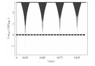
Figure 2: Plot of the envelope of $\textrm{Log}_{10}(\textrm{F}/\textrm{F}_{\textrm{SQL}})$ (rapidly oscillating at the angular frequency $\Omega$) versus the interaction time, at four different values of damping, $\gamma=\{0.01,0.1,1\}$ Hz, corresponding to increasingly darker grey curves. The other parameters are given by Table 1, while the mirror temperature is T = 0 and there is no initial entanglement between the sideband modes, $s$ = 0. The dashed line represents the SQL.

As the interaction time increases, the minimum detectable force at the local minima increases as well, because the effect of damping becomes more and more important at longer times. As a consequence, the first minimum at $t_{1}\simeq\pi/\Theta$, ($t_{1}\simeq 15$ ms with the parameter values of Table 1) corresponds to the best possible sensitivity attainable with the device at issue. In typical situations, the time of arrival of the slowly varying force to be detected is unknown (consider for example the case of the tidal force of a gravitational wave). In such a case, the best detection strategy corresponds to a pulsed regime, in which a precise temporal switch fixes a pulse duration exactly equal to $t_{1}$ for the impinging laser, with a repetition rate of the order of the damping frequency $\gamma$.

The dashed line in Fig. 2 represents the SQL, obtained when $\textrm{F}/\textrm{F}_{\textrm{SQL}}=1$. It is apparent that for sufficiently low values of $\gamma$ the sensitivity goes beyond the SQL. However, when $\gamma$ assumes the more realistic value of $1$ Hz (darkest grey in the figure) the entanglement created by the dynamics is no more sufficient to go below the SQL, in none of its minima. However, as shown by Ref. FMT04 , there is a further resource that can be exploited in order to beat the SQL, i.e., the two-mode squeezing of the initial state of Eq. (24). This factor represents a sort of “static” entanglement that can add its effect to that of the dynamically generated entanglement between the sidebands and is able to increase significantly the sensitivity of the apparatus.

Hereafter we concentrate on the first minimum of the minimum detectable force of Fig. 2, that is we fix $t_{1}\simeq\pi/\Theta$.

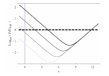
Figure 3: Plot of $\textrm{Log}_{10}(\textrm{F}/\textrm{F}_{\textrm{SQL}})$ versus the two-mode squeezing factor $s$, at four different values of damping, $\gamma=\{0.01,0.1,1,10\}$ Hz, corresponding to increasingly darker grey curves. The dashed line represents the SQL. The other parameters are given by Table 1, while the mirror temperature is T = 0.

In Fig. 3 the force sensitivity is plotted versus the two-mode squeezing factor $s$, for four different values of the damping rate, $\gamma=\{0.01,0.1,1,10\}$ Hz, and again at zero temperature. The dashed line is the SQL. As expected, the force detection sensitivity worsens for increasing damping. As shown by Fig. 2, when $s=0$ and $\gamma=1$ Hz the sensitivity is above the SQL. However it goes below the SQL in correspondence of a two-mode squeezing coefficient $s\simeq 1.5$ (a squeezing of about $13$ dB). Interestingly enough, at fixed $\gamma$, the minimum detectable force is not a monotonically decreasing function of $s$, but it has a minimum, meaning that for each $\gamma$ there is an optimal two-mode squeezing value maximizing the force detection sensitivity. This feature was lacking in Ref. FMT04 , in which the best possible squeezing was the highest one, and is a consequence of the inclusion of damping and noise in the model. From a physical point of view, this means that once that the interaction time $t_{1}$ is fixed, the input entanglement and the dynamically generated entanglement interfere in a nontrivial way, so that the optimal sensitivity is achieved at a finite value of two-mode squeezing $s$.

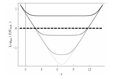
Figure 4: Plot of $\textrm{Log}_{10}(\textrm{F}/\textrm{F}_{\textrm{SQL}})$ versus the two-mode squeezing factor $s$, at four different values of temperature, $T=\{0,0.03,3,300\}$ K, corresponding to increasingly darker grey curves. The dashed line represents the SQL. The other parameters are given by Table 1.

Finally we study the temperature dependence of the sensitivity of the detection scheme. In Fig. 4 we show the behavior of the minimum detectable force versus $s$, at four different values of the temperature, $T=\{0,0.03,3,300\}$ K and at fixed damping, $\gamma=1$ Hz, while the other parameters are again those reported in Table 1. We see that up to mirror temperatures of the order of few Kelvin degrees, a nonzero value of the input two-mode squeezing is able to compensate the detrimental effects of damping and thermal noise acting on the mirror and one can achieve a detection sensitivity better than the SQL. This becomes impossible at room temperature, where the minimum detectable force becomes larger than the SQL, for any value of $s$.

V Conclusion

We have studied in detail the optomechanical scheme for the detection of weak forces proposed in Ref. FMT04 , based on the heterodyne measurement of a combination of two sideband modes of an intense driving laser, scattered by a vibrational mode of a highly reflecting mirror. In particular we have considered the dynamical effects of damping and thermal noise acting on the mirror vibrational mode, which were neglected in Ref. FMT04 . The dynamics of the system is characterized by a bilinear coupling of the two optical sidebands with the vibrational mode, which is able to generate significant entanglement between the two sidebands for an appropriate duration of the driving laser pulse PM+03 ; FMT04 . This condition corresponds to the highest signal-to-noise ratio for the detection of a slowly varying mechanical force acting on the mirror which, for extremely low values of the mirror damping and temperature, can be better than the SQL for the detection of a force BK92 . At more realistic values of damping and temperatures, the minimum detectable force becomes larger than the SQL and the dynamically generated entanglement is no more able to counteract the effects of damping and thermal noise. However, we show that the presence of additional entanglement in the input state of the two sidebands may improve the performance of the detection scheme and one can go significantly below the SQL, even in the presence of non-negligible mirror damping and not too low temperatures. For example the SQL can be beaten by adopting a vibrational mode with a mechanical quality factor $\Omega/\gamma\simeq 10^{7}$ and at temperatures around $3$ K.

This work has been supported by the European Commission through the Integrated Project ‘Scalable Quantum Computing with Light and Atoms’ (SCALA), Contract No 015714, ‘Qubit Applications’ (QAP), Contract No 015848, funded by the IST directorate, and the Ministero della Istruzione, dell’Università e della Ricerca (PRIN-2005024254 and FIRB-RBAU01L5AZ).

References

- (1) C. Bradaschia et al., Nucl. Instrum. Methods Phys. Res. A 289, 518 (1990); A. Abramovici et al., Science 256, 325 (1992).
- (2) J. Mertz et al., Appl. Phys. Lett. 62, 2344 (1993); T.D. Stowe et al., ibid. 71, 288 (1997).
- (3) C. M. Caves, Phys. Rev. D 23, 1693 (1981); M. T. Jaekel and S. Reynaud, Europhys. Lett. 13, 301 (1990).
- (4) V. B. Braginsky and F. Ya Khalili, Quantum Measurements (Cambridge University Press, Cambridge, England, 1992).
- (5) X. M. H. Huang et al., Nature (London) 421, 496 (2003); R. G. Knobel and A. N. Cleland, Nature (London) 424, 291 (2003); M. D. LaHaye et al., Science 304, 74 (2004).
- (6) J. L. Arlett, J. R. Maloney, B. Gudlewski, and M. L. Roukes, Nano Lett. 6, 1000 (2006).
- (7) R. F. Service, Science 312, 683 (2006).
- (8) D. Vitali, S. Mancini, and P. Tombesi, Phys. Rev. A 64, 051401(R) (2001); D. Vitali, S. Mancini, L. Ribichini, and P. Tombesi, Phys. Rev. A 65, 063803 (2001); J. M. Courty, A. Heidmann, and M. Pinard, Phys. Rev. Lett. 90, 083601 (2003); O. Arcizet, T. Briant, A. Heidmann, and M. Pinard, Phys. Rev. A 73, 033819 (2006).
- (9) R. Fermani, S. Mancini and P. Tombesi, Phys. Rev. A 70, 045801 (2004).
- (10) H. Rokhsari, T. J. Kippenberg, T. Carmon, and K. J. Vahala, Optics Express 13, 5293 (2005).
- (11) S. Pirandola, S. Mancini, D. Vitali and P. Tombesi, Phys. Rev. A 68, 062317 (2003).
- (12) S. Pirandola S. Mancini, D. Vitali and P. Tombesi, J. Mod. Opt. 51, 901 (2004).
- (13) C. W. Gardiner and P. Zoller, Quantum Noise, (Springer, Berlin, 2000).
- (14) M. Pinard et al., Eur. Phys. J. D 7, 107 (1999).
- (15) V. Giovannetti and D. Vitali, Phys. Rev. A 63, 023812 (2001).
- (16) C. W. Gardiner and P. Zoller, Quantum Noise, (Springer, Berlin, 2000), p. 71.
- (17) H. P. Yuen and J. H. Shapiro, IEEE Trans. Inf. Theory IT-26, 78 (1980).
- (18) J. N. Hollenhorst, Phys. Rev. D 19, 1669 (1979).
- (19) D. F. Walls and G. J. Milburn, Quantum Optics, (Springer, Berlin, 1994)