A minimum-disturbing quantum state discriminator

Abstract

We propose two experimental schemes for quantum state discrimination that achieve the optimal tradeoff between the probability of correct identification and the disturbance on the quantum state.

1. Introduction

Indistinguishability of nonorthogonal states is a basic feature of quantum mechanics that has deep implications in many areas, as quantum computation and communication, quantum entanglement, cloning, and cryptography. Since the pioneering work of Helstrom [1] on quantum hypothesis testing, the problem of discriminating nonorthogonal quantum states has received a lot of attention [2], with some experimental verifications as well [3]. The most popular scenarios are: $i)$ the minimum-error probability discrimination [1], where each measurement outcome selects one of the possible states and the error probability is minimized; $ii)$ the optimal unambiguous discrimination [4], where unambiguity is paid by the possibility of getting inconclusive results from the measurement; $iii)$ the minimax strategy [5] where the smallest of the probabilities of correct detection is maximized. Stimulated by the rapid developments in quantum information theory, the problem of discrimination has been addressed also for bipartite quantum states, along with the comparison of global strategies where unlimited kind of measurements is considered, with the scenario of LOCC scheme, where only local measurements and classical communication are allowed [6]. The concepts of nonorthogonality and distinguishability can be applied also to quantum operations, namely all physically allowed transformations of quantum states, and some work has been devoted to the problem of discriminating unitary transformations [7] and more general quantum operations [8].

The quantum indistinguishability principle is closely related to another very popular, yet often misunderstood, principle (formerly known as Heisenberg principle [9, 10, 11]): it is not possible to extract information from a quantum system without perturbing it somehow. In fact, if the experimenter could gather information about an unknown quantum state without disturbing it at all, even if such information is partial, by performing further non-disturbing measurements on the same system, he could finally determine the state, in contradiction with the indistinguishability principle [12].

Actually, there exists a precise tradeoff between the amount of information extracted from a quantum measurement and the amount of disturbance caused on the system, analogous to Heisenberg relations holding in the preparation procedure of a quantum state. Quantitative derivations of such a tradeoff have been obtained in the scenario of quantum state estimation [13, 14]. The optimal tradeoff has been derived in the following cases: in estimating a single copy of an unknown pure state [11], many copies of identically prepared pure qubits [15], a single copy of a pure state generated by independent phase-shifts [16], an unknown maximally entangled state [17], an unknown coherent state [18] and Gaussian state [19], and an unknown spin coherent state [20].

Experiment realization of minimal disturbance measurements has been also reported [18, 21].

In the present paper we review the characterization of the tradeoff relation in quantum state discrimination of Ref. [22], and suggest an experimental realization of the minimum-disturbing measurement. In this case, an unknown quantum state is chosen with equal a priori probability from a set of two non orthogonal pure states, and the error probability of the discrimination is allowed to be suboptimal (thus intuitively causing less disturbance with respect to the optimal discrimination). A measuring strategy that achieves the optimal tradeoff is shown to smoothly interpolate between the two limiting cases of maximal information extraction and no measurement at all. The issue of the information-disturbance tradeoff for state discrimination can become of practical relevance for posing general limits in information eavesdropping and for analyzing security of quantum cryptographic communications.

After briefly reviewing the optimal information-disturbance tradeoff in quantum state discrimination and the corresponding measurement instrument, we analyze two possible experimental realization of the minimum-disturbing measurement.

2. Information-disturbance tradeoff in quantum state discrimination

Typically, in quantum state discrimination we are given two (fixed) non orthogonal pure states $\psi_{1}$ and $\psi_{2}$, with a priori probabilities $p_{1}$ and $p_{2}=1-p_{1}$, and we want to construct a measurement discriminating between the two. We can describe a measurement by means of an instrument [23], namely, a collection of completely positive maps $\{\mathcal{E}_{i}\}$, labelled by the measurement outcomes $\{i\}$. Using the Kraus decomposition [24], one can always write $\mathcal{E}_{i}(\rho)=\sum_{k}E^{(i)}_{k}\rho E^{(i){\dagger}}_{k}$. In the case the sum comprises just one term, namely, $\mathcal{E}_{i}(\rho)=E_{i}\rho E^{\dagger}_{i}$, the map $\mathcal{E}_{i}$ is called pure, since it maps pure states into pure states. The trace $\operatorname{Tr}[\mathcal{E}_{i}(\rho)]=\operatorname{Tr}[\Pi_{i}\rho]$, where $\Pi_{i}=\sum_{k}E^{(i){\dagger}}_{k}E^{(i)}_{k}$ is a positive operator associated to the $i$-th outcome, provides the probability that the measurement performed on a quantum system described by the density matrix $\rho$ gives the $i$-th outcome. The posterior (or reduced) state after the measurement is given by $\rho_{i}=\mathcal{E}_{i}(\rho)/\operatorname{Tr}[\mathcal{E}_{i}(\rho)]$. The averaged reduced state—coming from ignoring the measurement outcome—is simply obtained using the trace-preserving map $\mathcal{E}=\sum_{i}\mathcal{E}_{i}$. The trace-preservation constraint for $\mathcal{E}$ implies that the set of positive operators $\{\Pi_{i}\}$ is actually a positive operator-valued measure (POVM), satisfying the completeness condition $\sum_{i}\Pi_{i}=I$.

Quantum state discrimination is then performed by a two-outcome instrument $\{\mathcal{E}_{1},\mathcal{E}_{2}\}$ whose capability of discriminating between $\psi_{1}$ and $\psi_{2}$ can be evaluated by the average success probability

$$P(\{\mathcal{E}_{1},\mathcal{E}_{2}\})=\sum_{i=1}^{2}p_{i}\operatorname{Tr}[\mathcal{E}_{i}(|\psi_{i}\rangle\langle\psi_{i}|)]=\sum_{i=1}^{2}p_{i}\operatorname{Tr}[\Pi_{i}|\psi_{i}\rangle\langle\psi_{i}|].$$ (1)

Notice that $P$ actually depends only on the POVM $\{\Pi_{i}\}$. The probability $P$ quantifies the amount of information that the instrument $\{\mathcal{E}_{1},\mathcal{E}_{2}\}$ is able to extract from the ensemble $\{p_{1},\psi_{1};p_{2},\psi_{2}\}$. Among all instruments achieving average success probability $\bar{P}$ (the bar over $P$ means that we fix the value of $P$), we are interested in those minimizing the average disturbance caused on the unknown state, that we evaluate in terms of the average fidelity, namely,

$$D(\{\mathcal{E}_{1},\mathcal{E}_{2}\},\bar{P})=1-\sum_{i=1}^{2}p_{i}\langle\psi_{i}|\mathcal{E}(|\psi_{i}\rangle\langle\psi_{i}|)|\psi_{i}\rangle.$$ (2)

Differently from $P$, the disturbance $D$ strongly depends on the particular form of the instrument $\{\mathcal{E}_{i}\}$. This means that there exist many different instruments achieving the same $P$, but giving different values of $D$. Let

$$\bar{D}(\bar{P})=\min_{\{\mathcal{E}_{1},\mathcal{E}_{2}\}}D(\{\mathcal{E}_{1},\mathcal{E}_{2}\},\bar{P})$$ (3)

be the disturbance produced by the least disturbing instrument that discriminates $\psi_{1}$ from $\psi_{2}$ with average success probability $\bar{P}$. Intuitive arguments suggest that the larger is $\bar{P}$, the larger must correspondingly be $\bar{D}$ (i. e., the larger is the amount of information extracted, the larger is the disturbance caused by the measurement). The precise derivation of the optimal tradeoff $\bar{D}(\bar{P})$ has been obtained in Ref. [22], along with the corresponding optimal measurement, for equal a priori probabilities, i. e. $p_{1}=p_{2}=1/2$. In the following we briefly review the main results.

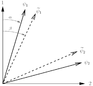
Let us start reviewing the case of the measurement maximizing $P$. Notice that, given two generally non orthogonal pure states $\psi_{1}$ and $\psi_{2}$, it is always possible to choose an orthonormal basis $\{|1\rangle,|2\rangle\}$, placed symmetrically around $\psi_{1}$ and $\psi_{2}$ (see Fig. 1), on which both states have real components, namely

$$\begin{split}&|\psi_{1}\rangle=\cos\alpha\;|1\rangle+\sin\alpha\;|2\rangle,\\ &|\psi_{2}\rangle=\sin\alpha\;|1\rangle+\cos\alpha\;|2\rangle,\end{split}$$ (4)

and fidelity $f=|\langle\psi_{1}|\psi_{2}\rangle|=\sin 2\alpha$. In this case, it is known [1] that the maximum achievable $P$ is given by

$$P_{\textrm{opt}}=\cos^{2}\alpha,$$ (5)

which is obtained by the orthogonal von Neumann measurement $\{|1\rangle\langle 1|,|2\rangle\langle 2|\}$.

Fig. 1: Helstrom’s scheme to optimally discriminate between to non orthogonal states $\psi_{1}$ and $\psi_{2}$. The orthogonal axes $1$ and $2$ correspond to the von Neumann measurement that achieves the optimal discrimination probability (5). According to the measurement outcome, $\widetilde{\psi}_{1}$ and $\widetilde{\psi}_{2}$ are the states to be prepared, in order to minimize the disturbance.

The instrument achieving $P_{\textrm{opt}}$, that minimizes the disturbance $D$ is given by

$$\mathcal{E}_{i}(\rho)=U_{i}|i\rangle\langle i|\rho|i\rangle\langle i|U^{\dagger}_{i},\qquad i=1,2,$$ (6)

where $U_{1}$ is the unitary operator

$$U_{1}=\begin{pmatrix}\cos\beta&\sin\beta\\ -\sin\beta&\cos\beta\end{pmatrix},$$ (7)

$U_{2}=U_{1}^{\dagger}$, and $\beta$ satisfies the equation [10, 22]

$$\tan 2\beta=\frac{\tan 2\alpha}{\cos 2\alpha}.$$ (8)

Equation (6) represents a measure-and-prepare realization: the observable $|i\rangle\langle i|$ is measured and, depending on the outcome, the quantum state $|\widetilde{\psi}_{i}\rangle=U_{i}|i\rangle$ is prepared. The states $|\widetilde{\psi}_{i}\rangle$ are symmetrically tilted with respect to the $|\psi_{i}\rangle$’s, see Fig. 1.

The presence of the tilt $\beta$ can be understood by noticing that minimum error discrimination can never be error-free for non orthogonal states. Even using the optimal Helstrom’s measurement, there is always a non zero error probability, and, the closer the input states are to each other, the smaller the success probability is. Hence, it is reasonable that, the closer the input states are, the less “trustworthy” the measurement outcome is, and the average disturbance is minimized by cautiously preparing a new state that actually is a coherent superpositions of both hypotheses $\psi_{1}$ and $\psi_{2}$. The minimum disturbance for Helstrom’s optimal measurement is given by

$$D_{\textrm{opt}}=\frac{4-\sqrt{14+2\cos 8\alpha}}{8}.$$ (9)

Notice that $D_{\textrm{opt}}$ reaches its maximum for $\alpha=\pi/8$, namely, when $\psi_{1}$ and $\psi_{2}$ are “unbiased” with respect to each other ($|\langle\psi_{1}|\psi_{2}\rangle|^{2}=1/2$).

By allowing a suboptmal discrimination, with success probability $P<P_{\textrm{opt}}$, one can cause less disturbance. In this case, by parametrizing the average success probability thorugh a control parameter $t$ as follows

$$P_{t}=tP_{\textrm{opt}}+\frac{1-t}{2}=t\cos^{2}\alpha+\frac{1-t}{2},$$ (10)

with $0\leq t\leq 1$, one can search, among all possible measurements achieving $P_{t}$, the one minimizing the disturbance $D(P_{t})$. It turns out that, for any value of $P_{t}$, the minimum disturbance $D_{t}$ is achieved by the pure instrument $\mathcal{E}_{i}^{(t)}(\rho)=E_{i}^{(t)}\rho E_{i}^{(t){\dagger}}$, where [22]

$$\begin{split}E_{1}^{(t)}&=U(t)\left(\frac{\sqrt{1-\gamma}}{2}\sigma_{z}+\frac{\sqrt{1+\gamma}}{2}I\right),\\ E_{2}^{(t)}&=U^{\dagger}(t)\left(-\frac{\sqrt{1-\gamma}}{2}\sigma_{z}+\frac{\sqrt{1+\gamma}}{2}I\right),\end{split}$$ (11)

with $\gamma=\sqrt{1-t^{2}}$. The unitary operator $U(t)$ in the above equation generalizes that in Eq. (7) as follows

$$U(t)=\begin{pmatrix}\cos\beta_{t}&\sin\beta_{t}\\ -\sin\beta_{t}&\cos\beta_{t}\end{pmatrix},$$ (12)

with

$$\tan 2\beta_{t}=\frac{t\sin 2\alpha}{\cos^{2}2\alpha+\gamma\sin^{2}2\alpha}.$$ (13)

It follows that every instrument that achieves average success probability $P_{t}$ must cause at least an average disturbance

$$D_{t}=\frac{1}{2}\left(1-t\sin 2\alpha\sin 2\beta_{t}\right)+\frac{\cos 2\beta_{t}}{4}\left[\gamma(\cos 4\alpha-1)-\cos 4\alpha-1\right].$$ (14)

Just by varying the control parameter $t$, it is possible to smoothly move between the limiting cases. For $t=0$, we obtain the identity map, that is, the no-measurement case. For $t=1$, we obtain Helstrom’s instrument in Eq. (6), and Eq. (13) reproduces the tilt given in Eq. (8). However, the crucial difference between Helstrom’s limit ($t=1$) and the intermediate cases is that, for $t<1$, the optimal instrument cannot be interpreted by means of a measure-and-prepare scheme, and the unitaries $U(t)$ and $U^{\dagger}(t)$ in Eq. (11) represent feedback rotations for outcomes $1$ and $2$.

By eliminating the parameter $t$ from Eqs. (10) and (14), one can obtain the optimal tradeoff between information and disturbance, for any value of $\alpha$ [10, 22].

3. Experimental schemes for the minimum-disturbing measurement

In this section we want to show two experimental schemes for the realization of the minimum-disturbing measurement. The two-level input system is encoded on photons degrees of freedom. Since we are interested not only in the success probability but also in the posterior state of the system after the measurement, we have to focus on indirect measurement schemes, in which the system is previously made interact with a probe, and, after such interaction, a projective measurement is performed on the probe. The mathematical parameter $t$ controlling the tradeoff in Eq. (10) can then be put in correspondence with a physical parameter controlling the strength of the interaction between the system and the probe. The case $t=0$ means that the interaction is actually factorized and that the subsequent measurement on the probe does not provide any information about the system and the latter is completely unaffected by the probe’s measurement. This is precisely the no-measurement case. On the contrary, $t=1$ identifies a completely entangling interaction, or, in other words, a situation in which a measurement on the probe gives the largest amount of information about the system, consequently causing the largest disturbance. In the following, two possible settings are discussed: the first one, which is deterministic and involves the dual-rail representation of qubits [25], and the second one which is probabilistic and involves the qubit encoding on the polarization state of a single photon.

3.1. Deterministic scheme ($t\ll 1$)

In Ref. [25] it is shown how to achieve a maximally entangling gate of the C-NOT type, i. e.

$$|i\rangle_{s}|1\rangle_{p}\mapsto|i\rangle_{s}|i\rangle_{p},\qquad i=1,2$$ (15)

by combining, in the dual-rail representation of qubits, two Hadamard gates with a non-linear interaction caused by a Kerr medium coupling the two modes $s$ (system) and $p$ (probe). More explicitly, by varying the interaction time (or length) between the system mode and the probe mode inside the Kerr medium, it is possible to achieve the following unitary evolution:

$$U(\phi)=\begin{pmatrix}1&0&0&0\\ 0&1&0&0\\ 0&0&\frac{1+e^{i\phi}}{2}&\frac{1-e^{i\phi}}{2}\\ 0&0&\frac{1-e^{i\phi}}{2}&\frac{1+e^{i\phi}}{2}\end{pmatrix}.$$ (16)

The two limiting cases correspond to $\phi=0$ for which $U(0)=I$, and $\phi=\pi$ for which $U(\pi)$ realizes a perfect C-NOT gate. Then, to measure the von Neumann observable $\{|1\rangle\langle 1|,|2\rangle\langle 2|\}$ on the probe is equivalent to apply the instrument in Eq. (11) onto the system, with $t=\sin^{2}(\phi/2)$. The feedback unitary rotation (12) can be subsequently applied conditional to the probe measurement outcome.

This scheme is deterministic, that is, no events have to be discarded. However, approaching the limiting value $\phi=\pi$ (or, equivalently, $t=1$) is quite hard, since too large nonlinearity is needed  [26]. Hence, such a setup can be useful only for regimes with $t\ll 1$.

3.2. Probabilistic scheme

The second proposal is a modification of the setup already used in Ref. [21] to experimentally realize a universal minimum-disturbing measurement. With respect to Ref. [21], only the feedback rotations are different. This setup has the great advantage of being completely achievable by linear optics. In order to entangle the system with the probe, it needs an entangling measurement to be performed on the joint system-probe–state. Such a measurement is in fact a parity check, namely a measurement of the observable

$$\{P_{y}=|1\rangle\langle 1|_{s}\otimes|1\rangle\langle 1|_{p}+|2\rangle\langle 2|_{s}\otimes|2\rangle\langle 2|_{p},\ \ P_{n}=I-P_{y}\}.$$ (17)

However, since the outcome “$n$” corresponds to a situation in which the input photon and the probe photon are indistinguishable, we are forced to post-select just one half of the events, discarding those corresponding to the outcome $n$. A part of this major drawback, limiting the actual usefulness of such a measuring instrument in practical application, using this setup it is possible to explore the whole range of the parameter values $t\in[0,1]$, contrarily to what happens using non-linear media.

References

- [1] C. W. Helstrom, Quantum Detection and Estimation Theory (Academic Press, New York, 1976).
- [2] For a recent review, see J. Bergou, U. Herzog, and M. Hillery, Quantum state estimation, Lecture Notes in Physics Vol. 649 (Springer, Berlin, 2004), p. 417; A. Chefles, ibid., p. 467.
- [3] B. Huttner, A. Muller, J. D. Gautier, H. Zbinden, and N. Gisin, Phys. Rev. A 54, 3783 (1996); S. M. Barnett and E. Riis, J. Mod. Opt. 44, 1061 (1997); R. B. M. Clarke, A. Chefles, S. M. Barnett, and E. Riis, Phys Rev A. 63, 040305(R) (2001); R. B. M. Clarke, V. M. Kendon, A. Chefles, S. M. Barnett, E. Riis, and M. Sasaki, Phys. Rev. A 64, 012303 (2001); M. Mohseni, A. M. Steinberg, and J. A. Bergou, Phys. Rev. Lett. 93, 200403 (2004).
- [4] I. D. Ivanovic, Phys. Lett. A 123, 257 (1987); D. Dieks, Phys. Lett. A 126, 303 (1988); A. Peres, Phys. Lett. A 128, 19 (1988); G. Jaeger and A. Shimony, Phys. Lett. A 197, 83 (1995); A. Chefles, Phys. Lett. A 239, 339 (1998).
- [5] G. M. D’Ariano, M. F. Sacchi, and J. Kahn, Phys. Rev A 72, 032310 (2005).
- [6] J. Walgate, A. J. Short, L. Hardy, and V. Vedral, Phys. Rev. Lett. 85, 4972 (2000); S. Virmani, M. F. Sacchi, M. B. Plenio, and D. Markham, Phys. Lett. A 288, 62 (2001); Y.-X. Chen and D. Yang, Phys. Rev. A 64, 064303 (2001); 65, 022320 (2002); Z. Ji, H. Cao, and M. Ying, Phys. Rev. A 71, 032323 (2005).
- [7] A. M. Childs, J. Preskill, and J. Renes, J. Mod. Opt. 47, 155 (2000); A. Acín, Phys. Rev. Lett. 87, 177901 (2001); G. M. D’Ariano, P. Lo Presti, and M. G. A. Paris, Phys. Rev. Lett. 87, 270404 (2001).
- [8] M. F. Sacchi, Phys. Rev. A 71, 062340 (2005).
- [9] W. Heisenberg, Zeitsch. Phys. 43, 172 (1927); M. O. Scully, B.-G. Englert, and H. Walther, Nature 351, 111 (1991); B.-G. Englert, Phys. Rev. Lett. 77, 2154 (1996); C. A. Fuchs and K. Jacobs, Phys. Rev. A 63, 062305 (2001); H. Barnum, e-print quant-ph/0205155; G. M. D’Ariano, Fortschr. Phys. 51, 318 (2003); M. Ozawa, Ann. Phys. 311, 350 (2004); L. Maccone, Phys. Rev. A 73, 042307 (2006).
- [10] C. A. Fuchs, Fortschr. Phys. 46, 535 (1998).
- [11] K. Banaszek, Phys. Rev. Lett. 86, 1366 (2001).
- [12] G. M. D’Ariano and H. P. Yuen, Phys. Rev. Lett. 76, 2832 (1996).
- [13] A. S. Holevo, Probabilistic and Statistical Aspects of Quantum Theory (North Holland, Amsterdam, 1982).
- [14] S. Massar and S. Popescu, Phys. Rev. Lett. 74, 1259 (1995); R. Derka, V. Buzek, and A. K. Ekert, Phys. Rev. Lett. 80, 1571 (1998); J. I. Latorre, P. Pascual, and R. Tarrach, Phys. Rev. Lett. 81, 1351 (1998); G. Vidal, J. I. Latorre, P. Pascual, and R. Tarrach, Phys. Rev. A 60, 126 (1999); A. Acín, J. I. Latorre, and P. Pascual, Phys. Rev. A 61, 022113 (2000); G. Chiribella, G. M. D’Ariano, P. Perinotti, and M. F. Sacchi, Phys. Rev. A 70, 062105 (2004); G. Chiribella, G. M. D’Ariano, and M. F. Sacchi, Phys. Rev. A 72, 042338 (2005).
- [15] K. Banaszek and I. Devetak, Phys. Rev. A 64, 052307 (2001).
- [16] L. Mišta Jr., J. Fiurášek, and R. Filip, Phys. Rev. A 72, 012311 (2005).
- [17] M. F. Sacchi, Phys. Rev. Lett. 96, 220502 (2006).
- [18] U. L. Andersen, M. Sabuncu, R. Filip, and G. Leuchs, Phys. Rev. Lett. 96, 020409 (2006).
- [19] M. G. Genoni and M. G. A. Paris, Phys. Rev. A 74, 012301 (2006).
- [20] M. F. Sacchi, unpublished.
- [21] F. Sciarrino, M. Ricci, F. De Martini, R. Filip, and L. Mišta Jr., Phys. Rev. Lett. 96, 020408 (2006).
- [22] F. Buscemi and M. F. Sacchi, quant-ph/0610196 (to appear on Phys. Rev. A).
- [23] E. B. Davies and J. T. Lewis, Commun. Math. Phys. 17, 239 (1970); M. Ozawa, J. Math. Phys. 5, 848 (1984).
- [24] K. Kraus, States, Effects, and Operations: Fundamental Notions in Quantum Theory, Lect. Notes Phys. 190 (Springer-Verlag, 1983).
- [25] M A Nielsen and I L Chuang, Quantum Information and Computation (Cambridge University Press, Cambridge, 2000). See in particular Section 7.4.2.
- [26] M. Fleischhauer, A. Imamoglu, and J. P. Marangos, Rev. Mod. Phys. 77, 633 (2005).