Dissipation Effects in Hybrid Systems

Abstract

The dissipation effect in a hybrid system is studied in this Letter. The hybrid system is a compound of a classical magnetic particle and a quantum single spin. Two cases are considered. In the first case, we investigate the effect of the dissipative quantum subsystem on the motion of its classical partner. Whereas in the second case we show how the dynamics of the quantum single spin are affected by the dissipation of the classical particle. Extension to general dissipative hybrid systems is discussed.

Quantum and classical theories are distinguished both in terms of their state spaces and their dynamics. Quantum states can predict measurement results that can not be reconciled with predictions by classical states, such as violations of Bell’s inequalitiesbell64 . Dynamically, although quantum and classical evolution agree on sufficiently short time scalessakurai93 , the mean values of observables diverge after some characteristic timeberry79 . When they go to dissipative systems, quantum open systems may be described by the master equation, while the dissipative force proportional to the momentum of the particle may be introduced to obtain the equations of motion for dissipative classical systems. Then a question arises, in a hybrid system composed of a quantum subsystem and a classical subsystem, how to treat the dissipation effects? And what are the effects? This question became more important in the last years because of remarkable progresskoppens05 ; yamamoto03 made in experiments in quantum information processing, where the qubits have to be coupled to the macroscopic world for initialization, gating and readout. For example, in a typical flux qubit gate, microwave pulses are applied onto specific qubit of the sample. This requires many classical systems coupling to the qubits, which is thus a compound of quantum and classical subsystems.

Besides its experimental interest, it is of central importance on the scientific side. For a closed hybrid system, the quantum subsystem may be treated classically slichter90 ; berman02 or quantum mechanicallyzhang06 , depending on specific issues addressed. The formulism requires that the hybrid system can be described by a Hamiltonian. This requirement, however, is not feasible for subsystems that include dissipation, in particular, for the quantum dissipative subsystem. The so-called system-plus-reservoir approach is to consider the classical subsystem as a reservoir, leading to decoherence in the quantum subsystem. This approach, however, ignore the backaction of the quantum subsystem, and hence is inadequate to address some issues, for instance, in single spin detection by the magnetic-resonance-force microscopyrugar04 .

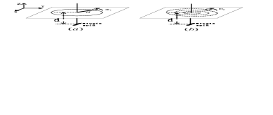
Figure 1: A schematic illustration of a single spin-$\frac{1}{2}$ particle interacting with a magnetic particle. ($a$) The magnetic particle is attached to a rigid cantilever and rotates in the $xy$ plane. The single spin placed beneath the plane with a distance of $d$ is dissipative due to coupling to its environment. ($b$) The magnetic particle moves dissipatively in the $xy$ plane, while the spin placed beneath the plane is decoherence free.

In this Letter, we present a method for dissipative hybrid systems. The hybrid system consists of a quantum subsystem, which is dynamically fast, and a slow classical subsystem. The presented representation is based on the fact that a quantum system possesses mathematically a canonical classical Hamiltonian structureheslot85 ; weinberg89 ; liu03 . In fact, this method was used in closed hybrid systems in zhang06 . To show the dissipation effects, we first consider the case where the quantum subsystem includes dissipation, while the classical subsystem does not dissipate. We examine the effect of the dissipative quantum system on the motion of the classical subsystem. The second case we consider is that only the classical subsystem in the hybrid system is dissipative. The dynamics as well as the adiabaticity of the quantum subsystem are examined. We find that large dissipation rates of the classical subsystem benefit the adiabatic evolution of the quantum subsystem, and the vector potential arised in the hybrid system tends to zero with the dissipation rate approaching infinity. On the other hand, the dissipative quantum subsystem produces a magnetic-like field in the slow classical subsystem. The strength of this field oscillates at intermediate values of the dissipation rate, and then approaches zero with large dissipation rates.

We shall use a simple hybrid system, which consists of a single spin coupling to a heavy magnetic particle, to show the idea. The assumption that the magnetic particle is dynamically slow with respect to the single spin is of relevance to the single spin detection by the magnetic-resonance-force microscopyrugar04 , where the cantilever plays the role of the slow classical subsystem. A schematic setup of the studied system was shown in figure 1. A magnetic particle with magnetic moment, ${\bf m}_{F}$, is attached to the cantilever tip (Fig. 1-(a)). The cantilever is rigid and rotates freely in the $xy$ plane. A single spin with magnetic moment $\vec{\mu}$ is placed beneath the plance with a distance of $d$. We shall show the effect of the dissipative quantum subsystem on the motion of the magnetic particle through this imagined setup. Whereas by the setup in Fig. 1-(b), we shall study the dissipation effect of the classical subsystem on the quantum subsystem. The difference of the two setups is that, in the setup in Fig. 1-(b), the magnetic particle may move freely in the $xy$ plane, i.e., there is not any rigid cantilever for the magnetic particle to be attached.

Consider the hybrid system sketched in Fig. 1-(a). The dynamics of the single spin-$\frac{1}{2}$ particle can be described by the master equation,

$$\dot{\rho}=-i[\hat{H}(\vec{q}_{b}),\rho]+\frac{\gamma}{2}\{2\sigma_{-}\rho\sigma_{+}-\rho\sigma_{+}\sigma_{-}-\sigma_{+}\sigma_{-}\rho\},$$ (1)

where $\hat{H}(\vec{q}_{b})=\mu\vec{B}(\vec{q}_{b})\cdot\vec{\sigma}$ denotes the system Hamiltonian of the quantum single spin, $\gamma$ stands for the spontaneous emission rate. $\sigma_{i},i=z,+,-$ are the Pauli matrices, and $\sigma_{z}=|e\rangle\langle e|-|g\rangle\langle g|$ ($|e\rangle$, denotes the state of spin-up, and $|g\rangle$ spin-down). We shall denote $H_{b}(\vec{p}_{b},\vec{q}_{b})$ the Hamiltonian of the heavy classical subsystem $b$ that is dynamically slow, and $\vec{p}_{b},\vec{q}_{b}$ are its momenta and coordinates, respectively. The dependence of $\hat{H}_{a}(\vec{q}_{b})$ on $\vec{q}_{b}$ indicates the coupling between the two subsystems. The magnetic field acting on the single spin from the classical magnetic particle is given by ($\vec{q}_{b}=\{x,y,d\}$) zhang06

$$\vec{B}(\vec{q}_{b})=\{B_{x},B_{y},B_{z}\}=-\frac{\mu_{0}m_{F}\{3dx,3dy,2d^{2}-a^{2}\}}{4\pi(d^{2}+a^{2})^{5/2}},$$ (2)

where $a=\sqrt{x^{2}+y^{2}}$ keeps fixed in this case. The key idea required to use the frameworkzhang06 ; heslot85 ; weinberg89 ; liu03 for the exact treatment of the hybrid system is to find an effective Hamiltonian for the quantum subsystem. The method for this purpose was first presented in yi01 , the idea is the following. The density matrix $\rho(t)$ of the open system can be mapped onto a pure state by introducing an ancilla. The dynamics of the open system is then described by a Schrödinger-like equation with an effective Hamiltonian that can be derived from the master equation. In this way the solution of the master equation can be obtained in terms of the evolution of the composite system by converting the pure state back to the density matrix. For the single spin particle under consideration, we may introduce the other spin-$\frac{1}{2}$ particle with energy levels labelled by $|e\rangle^{A}$ and $|g\rangle^{A}$ as the ancilla. In spirit of the effective Hamiltonian approach, a pure state for the composite system (the single spin plus the ancilla) may be constructed as

$$|\Psi_{\rho}(t)\rangle=\sum_{m,n=e,g}\rho_{mn}(t)|m\rangle|n\rangle^{A},$$ (3)

where $\rho_{mn}(t)$ are density matrix elements of the open system in the basis $\{|e\rangle,|g\rangle\}$, i.e., $\rho_{mn}(t)=\langle m|\rho(t)|n\rangle,m,n=e,g.$ With these notations, we may find an effective Hamiltonian ${\cal H}_{T}(\vec{q}_{b})$, such that the bipartite(the spin plus the ancilla) pure state $|\Psi_{\rho}(t)\rangle$ satisfies the following Schrödinger-like equation

$$i\frac{\partial}{\partial t}|\Psi_{\rho}(t)\rangle={\cal H}_{T}(\vec{q}_{b})|\Psi_{\rho}(t)\rangle.$$ (4)

To shorten the derivation, we write the master equation Eq.(1) as

$$i\frac{\partial}{\partial t}\rho(t)={\cal H}\rho(t)-\rho(t){\cal H}^{\dagger}+i\gamma\sigma_{-}\rho(t)\sigma_{+},$$ (5)

with ${\cal H}=\hat{H}_{a}(\vec{q}_{b})-i\frac{\gamma}{2}|e\rangle\langle e|.$ Substituting equation Eq.(3) together with Eq.(5) into Eq.(4), one finds after some algebra,

$${\cal H}_{T}(\vec{q}_{b})={\cal H}-{\cal H}^{A}+i\gamma\sigma_{-}^{A}\sigma_{-}.$$ (6)

Operators ${\cal H}$ and $\sigma_{-}$ are for the single spin, which take the same form as in Eq.(5), while ${\cal H}^{A}$ and $\sigma_{-}^{A}$ are operators for the ancilla defined by

$${}^{A}\langle m|\hat{O}^{A}|n\rangle^{A}=\langle n|\hat{O}^{\dagger}|m\rangle,m,n=e,g,$$ (7)

with $\hat{O}={\cal H},$ or $\sigma_{-}.$ This yields ${\cal H}^{A}(\vec{q}_{b})=\hat{H}^{A}(\vec{q}_{b})+\frac{i}{2}|e\rangle^{AA}\langle e|,$ $\hat{H}^{A}(\vec{q}_{b})=\mu\vec{B}(\vec{q}_{b})\cdot\vec{\sigma}^{A}$, and $\vec{\sigma}^{A}$ represents the Pauli matrix of the ancilla. The first two terms in the effective Hamiltonian ${\cal H}_{T}(\vec{q}_{b})$ describe the free evolution of the spin and ancilla, respectively, and the third term characterizes couplings between the spin and the ancilla.

When the quantum subsystem is dynamically fast and the classical subsystem is slow, a vector potential $\vec{A}$ is generated in the hybrid system zhang06 . This vector potential behaves like the familiar Berry phase in the quantum subsystem, while it enters the classical subsystem in terms of magnetic-like fields $\vec{b}=\nabla\times\vec{A}$. With these knowledge, the total Hamiltonian for the dissipative hybrid system can be expressed in a pure classical formulism,

$$\tilde{H}={\cal H}_{T}(\vec{I}_{a},\vec{q}_{b})+H_{b}(\vec{P}_{a}-\vec{A},\vec{q}_{b}),$$ (8)

where ${\cal H}_{T}(\vec{I}_{a},\vec{q}_{b})=\sum_{i=1}^{4}\lambda_{i}p_{i}$, $(\vec{I}_{b})_{i}=\hbar p_{i},$ $H_{b}(\vec{P}_{a}-\vec{A},\vec{q}_{b})$ stands for the Hamiltonian of the classical subsystem, $\lambda_{i}$ $(i=1,2,3,4)$ are the eigenvalues of the effective Hamiltonian ${\cal H}_{T}$, and $p_{j}$ is the probability of finding the bipartite system (the single spin plus the ancilla) on state yi06 ,

$$|\psi_{j}\rangle=\frac{1}{\sqrt{M_{j}}}(a_{j}|e\rangle|e\rangle^{A}+b_{j}|e\rangle|g\rangle^{A}+c_{j}|g\rangle|e\rangle^{A}+d_{j}|g\rangle|g\rangle^{A}).$$ (9)

Tedious but standard calculations show that under the adiabatic evolution in open systemssarandy05 (see also yi06 ) the vector potential and magnetic-like field are $\vec{A}=\{A_{x},A_{y},0\}$ and $\vec{b}=\{0,0,b_{z}\}$, with ($\lambda_{4}=0$)

$$A_{x} = -\hbar\sum_{j=1}^{3}\frac{p_{j}}{M_{j}}(C_{j}c_{j}-B_{j}b_{j})\frac{y}{a^{2}},$$

$$A_{y} = \hbar\sum_{j=1}^{3}\frac{p_{j}}{M_{j}}(C_{j}c_{j}-B_{j}b_{j})\frac{x}{a^{2}},$$

$$b_{z} = 2\hbar\sum_{j=1,2,3}\frac{p_{j}}{a^{2}M_{j}}(C_{j}c_{j}-B_{j}b_{j}),$$ (10)

where

$$M_{j} = A_{j}a_{j}+B_{j}b_{j}+C_{j}c_{j}+D_{j}d_{j},$$

$$a_{j} = -(2\cos\theta+\frac{1}{2}i\gamma+\lambda_{j}),$$

$$b_{j} = 2\sin\theta e^{i\phi},$$

$$c_{j} = \frac{2\sin\theta(2\cos\theta+\frac{1}{2}i\gamma+\lambda_{j})e^{-i\phi}}{2\cos\theta-\frac{1}{2}i\gamma-\lambda_{j}},$$

$$d_{j} = -a_{j},$$

$$A_{j} = -(2\cos\theta-\frac{1}{2}i\gamma+\lambda_{j}),$$

$$D_{j} = \frac{i\gamma-\lambda_{j}}{i\gamma+\lambda_{j}}A_{j},$$

$$B_{j} = \frac{\sin\theta e^{-i\phi}(D_{j}-A_{j})}{2\cos\theta+\frac{1}{2}i\gamma+\lambda_{j}},$$

$$C_{j} = \frac{\sin\theta e^{i\phi}(D_{j}-A_{j})}{2\cos\theta-\frac{1}{2}i\gamma-\lambda_{j}},$$

$$\cos\theta = \frac{B_{z}}{|\vec{B}|},\ \ \tan\phi=\frac{B_{y}}{B_{x}},$$ (11)

and $\lambda_{j}$ is given by,

$$(\lambda_{j} + \frac{i}{2}\gamma)^{3}+\frac{i}{2}\gamma(\lambda_{j}+\frac{i}{2}\gamma)^{2}-4(\lambda_{j}+\frac{i}{2}\gamma)$$ (12)

$$= 2i\gamma^{2}\cos^{2}\theta.$$

We choose $p_{1}=p_{2}=p_{3}=\frac{1}{3}$ to show the dependence of $Re(b_{z})$ (the real part of $b_{z}$) on the dissipation rate $\gamma$ and the distance $d$. The numerical results were presented in figure 2. We find from figure 2 that $Re(b_{z})$ decays with $d$ increasing. This is easy to understand, since $d$ represents the distance between the magnetic particle and the single spin. One can also see from figure 2 that the dependence of $Re(b_{z})$ on $\gamma$ is a oscillating function. It arrives at its maximum with a nonzero $\gamma$, and then tends to zero with $\gamma\gg\mu|\vec{B}|.$

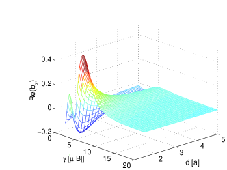
Figure 2: Real part of the magnetic-like field $Re(b_{z})$ versus the distance $d$ and the dissipation rate $\gamma.$ $p_{1}=p_{2}=p_{3}$ were chosen for this plot, and $Re(b_{z})$ was calculated in units of $\sqrt{m\mu|\vec{B}|}/a$.

Note that the dependence of the vector potential $\vec{A}$ on $\gamma$ and $d$ is similar to that of the magnetic-like field $\vec{b}$, hence $\vec{A}$ has the same feature as we presented above for $\vec{b}$. With this observation, the equation of motion for the magnetic particle (mass $m$) takes,

$$m\ddot{\bar{q}}_{b}=-\sum_{j}\frac{\partial\lambda_{j}}{\partial\vec{q}_{b}}p_{j}-m\Omega^{2}\vec{q}_{b}+\dot{\vec{q}}_{b}\times\vec{b},$$ (13)

where $\Omega$ is the frequency with that the classical particle circles. The first term on the right-hand side in Eq.(13) may be set to zero by properly choosing $p_{j}$. In this situation, the dissipation effect enters the classical particle through the magnetic-like field, and causes damping in the classical particle’s motion.

Now, we turn to study the second case illustrated in Fig.1-(b). In this case, the quantum subsystem is decoherence free and described by $\hat{H}_{a}(\vec{q}_{b})=\mu\vec{B}(\vec{q}_{b})\cdot\vec{\sigma},$ but the classical particle is subject to dissipations. We introduce a dissipative force $2\Gamma\dot{\vec{q}_{b}}$ to obtain the equations of motion in the form

$$\dot{\vec{p}_{b}} = -m\Omega^{2}\vec{q}_{b}-2\Gamma\frac{\vec{p}_{b}}{m},$$

$$\dot{\vec{q}_{b}} = \frac{\vec{p}_{b}}{m}.$$ (14)

This yields the well known damped solution

$$\vec{q}_{b}=e^{-\frac{\Gamma}{m}t}(\vec{A}\cos(\Omega_{0}t)+\vec{B}\sin(\Omega_{0}t)),$$ (15)

where $\Omega_{0}=\sqrt{\Omega^{2}-(\Gamma/m)^{2}}$, $\vec{A}$ and $\vec{B}$ depend on the initial condition of the magnetic particle. We are interested in the dynamics of the quantum subsystem under the influence of the damped magnetic particle. First, we study the effect of dissipation on the adiabaticity of the single spin. Assuming that $\vec{q}_{b}$ are just some fixed parameters, we obtain the instantaneous eigenstates for the quantum subsystem, $|+\rangle=\sin(\theta/2)e^{i\phi}|g\rangle+\cos(\theta/2)|e\rangle,$ and $|-\rangle=\cos(\theta/2)e^{i\phi}|g\rangle-\sin(\theta/2)|e\rangle,$ with $\cos\theta=B_{z}/|\vec{B}|,$ and $\tan\phi=B_{y}/B_{x}.$ The corresponding eigenenergies are $E_{+}=\mu|\vec{B}|,$ $E_{-}=-\mu|\vec{B}|,$ respectively. The adiabatic evolution of the single spin requires that

$$\kappa(\Gamma,t)=\frac{1}{4}|\dot{\theta}+i\Omega_{0}\sin\theta|\ll 1.$$ (16)

For $\Gamma=0,$ i.e., the magnetic particle is not dissipative, $\kappa(\Gamma,t)$ reduces to $\kappa(\Gamma,t)=\frac{1}{4}\Omega|\sin\theta|$, it depends on the frequency $\Omega$ and radius with that the magnetic particle circles. The dependence of $\kappa(\Gamma,t)$ on the damping rate $\Gamma$ and time $t$ was presented in figure 3.

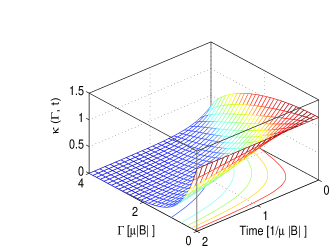
Figure 3: $\kappa(\Gamma,t)$ as a function of dissipation rate and time $t$. $\kappa(\Gamma,t)$ can be used to characterize the adiabaticity of the quantum subsystem. The parameters chosen are the same as in figure 2.

One can see from figure 3 that large dissipation rate $\Gamma$ would benefit the adiabatic evolution of the single spin. This can be understood by examining the effective frequency $\Omega_{0}$. Clearly, the larger the $\Gamma$, the smaller the $\Omega_{0}.$ From figure 3 we can also find that with time evolution, the adiabatic condition becomes easier to meet, this can be interpreted as the slowdown of the moving magnetic particle. Next, we study numerically the dissipation effect on the time evolution of the single spin, by calculating numerically the population on the state $|e\rangle.$ Extensive numerical simulations with the Hamiltonian $H_{a}(\vec{q}_{2})$ and the solution Eq. (15) have been performed, we find that for some fixed time points the population is a decay function of $\Gamma$, but for the other time points, the population increases first then decays (see figure 4). Note that the populations in the flat region in figure 4 are not zero. This damping effect revealed here is somewhat reminiscent of the quench effect in Landau-Zener like problems reported recently in damski .

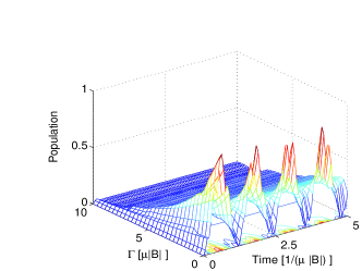
Figure 4: Population of the quantum subsystem on state $|e\rangle$. We have chosen $|g\rangle$ as the initial state for this plot.

The presented representation for the simple hybrid system can be easily extended to general hybrid systems. For an general open quantum subsystem, the dynamics may be described by the master equation,

$$i\frac{\partial}{\partial t}\rho(t) = [H^{\prime}(\vec{q}_{b}),\rho(t)]-\frac{i}{2}\sum_{k}\{L_{k}^{\dagger}(\vec{q}_{b})L_{k}(\vec{q}_{b})\rho(t)$$

$$+ \rho(t)L_{k}^{\dagger}(\vec{q}_{b})L_{k}(\vec{q}_{b})-2L_{k}(\vec{q}_{b})\rho(t)L_{k}^{\dagger}(\vec{q}_{b})\},$$

where $H^{\prime}(\vec{q}_{b})$ is a Hermitian Hamiltonian and $L_{k}(\vec{q}_{b})$ may be $\vec{q}_{b}$-dependent operators describing the system-environment interaction. The same procedure yields the effective Hamiltonian for the open quantum subsystem,

$${\cal H}_{T}^{\prime}(\vec{q}_{b})={\cal H}^{\prime}(\vec{q}_{b})-{\cal H}^{\prime,A}(\vec{q}_{b})+i\sum_{k}L_{k}^{A}(\vec{q}_{b})L_{k}(\vec{q}_{b}),$$ (18)

Where the operators with index $A$ are for the ancilla, which have the same definition as given above. In this way, we can discuss the dissipation effects in this hybrid system as we did in this Letter.

In conclusion, we have presented a first attempt at studying the dissipation effect in hybrid systems. The main results have been shown through a simple hybrid system, i.e., a compound of a classical magnetic particle and a quantum single spin. On one hand, the dissipative quantum subsystem affects the motion of its classical partner via magnetic-like fields. On the other hand, the damped classical particle changes the adiabaticity and the dynamics of the quantum single spin. The method presented here can be extended to general hybrid systems readily.

We thank Biao Wu for helpful discussions. This work was supported by EYTP of M.O.E, NSF of China (10305002 and 60578014).

References

- (1) J. S. Bell, Physics 1, 195 (1964).
- (2) J. J. Sakurai, Modern Quantum Mechanics ( Addison-Wesley, 1993).
- (3) M. V. Berry and N. L. Balazs, J. Phys. A: Math. Gen. 12, 625(1979).
- (4) F. H. L. Koppens et al., Science 309, 1346(2005); R. Hanson et al., Phys. Rev. Lett. 94, 196802(2005).
- (5) T. Yamamoto, Y. A. Pashkin, O. Astafiev, Y. Nakamura, J. S. Tsai, Nature (London) 425, 941(2003); I. Chiorescu, P. Bertet, K. Semba, Y. Nakamura, C. J. P. M. Harmans, J. E. Mooij, Nature (London) 431, 159(2004).
- (6) C. P. Slichter, Principles of magnetic resonance(Springer, Berlin 1990).
- (7) G. P. Berman, D. I. Kamener, and V. I. Tsifrinovich, Phys. Rev. A 66, 023405(2002).
- (8) Q. Zhang and B. Wu, e-print:quant-ph/0603073.
- (9) D. Rugar, R. Budakian, H. J. Mamin, and B. W. Chui, Nature 430, 329(2004).
- (10) A. Heslot, Phys. Rev. D 31, 1341(1985).
- (11) S. Weinberg, Ann. Phys. (N.Y.) 194, 336( 1989).
- (12) J. Liu, B. Wu, and Q. Niu, Phys. Rev. Lett. 90, 170404(2003).
- (13) X. X. Yi and S. X. Yu, J. Opt. B: Quantum Semiclass. 3, 272(2001).
- (14) X. X. Yi, D. M. Tong, L. C. Kwek, and C. H. Oh, e-print: quant-ph/0606203.
- (15) M. S. Sarandy, D. S. Lidar, Phys. Rev. A 71, 012331(2005); Phys. Rev. Lett. 95, 250503(1995).
- (16) B. Damski, W. H. Zurek, Phys. Rev. A 73, 063045(2006); W. H. Zurek, Nature (London) 317, 505(1985).