Entanglement in the above-threshold optical parametric oscillator

Abstract

We investigate entanglement in the above-threshold Optical Parametric Oscillator, both theoretically and experimentally, and discuss its potential applications to quantum information. The fluctuations measured in the subtraction of signal and idler amplitude quadratures are $\Delta^{2}\hat{p}_{-}=0.50(1)$, or $-3.01(9)$ dB, and in the sum of phase quadratures are $\Delta^{2}\hat{q}_{+}=0.73(1)$, or $-1.37(6)$ dB. A detailed experimental study of the noise behavior as a function of pump power is presented, and discrepancies with theory are discussed.

I Introduction

The Optical Parametric Oscillator (OPO) has been studied since the 1960’skingston62 ; grahamhaken68 . Already in the 1980’s it was recognized as an important tool in quantum optics, for the generation of squeezed states of light kimble ; heidmann . It was also recognized as a suitable system for the demonstration of continuous variable (CV) entanglement, by Reid and Drummond, in 1988 reiddrummprl88 , where above-threshold operation was considered. In the early 1990’s, CV entanglement was indeed demonstrated for the first time in an OPO, although operating below threshold kimbleepr . The OPO has since been used in several applications in CV quantum information vanloockbraunrmp05 ; bowen03 ; schori02 ; kimbleteleport ; entangswap04 . Entanglement in the above-threshold OPO, on the other hand, remained an experimental challenge until 2005, when it was first observed by Villar et al. prlentangtwinopo , and subsequently by two other groups optlettpeng ; pfisterentang .

Bipartite continuous variable entanglement can be demonstrated by a violation of the following inequality, obtained independently by Duan et al. dgcz and Simon simon :

$$\Delta^{2}\hat{p}_{-}+\Delta^{2}\hat{q}_{+}\geq 2\,,$$ (1)

where $\hat{p}_{-}=(\hat{p}_{1}-\hat{p}_{2})/\sqrt{2}$ and $\hat{q}_{+}=(\hat{q}_{1}+\hat{q}_{2})/\sqrt{2}$ are EPR-like operators constructed by combining operators of each subsystem. We choose $\hat{p}_{j}$ and $\hat{q}_{j}$, $j\in\{0,1,2\}$, as the amplitude and phase quadrature operators of the pump, signal and idler fields, respectively, which obey the commutation relations $[\hat{p}_{j},\hat{q}_{k}]=2i\delta_{jk}$. Any separable system must satisfy Eq. (1): violation is an unequivocal signature of entanglement.

Entanglement between the intense signal and idler beams generated by an above-threshold OPO can be physically understood as a consequence of energy conservation in the parametric process. On one hand, pump photons are converted into pairs of signal and idler photons, leading to strong intensity correlations; on the other hand, the sum of frequencies of signal and idler photons is fixed to the value of pump frequency, leading to phase anti-correlations. The difficulty of measuring phase fluctuations was largely responsible for the long time between the prediction and the first observation of entanglement in the above-threshold OPO. The technique we used to measure phase fluctuations consists of reflecting each field off an empty optical cavity, as explained in Ref optcomm04 .

The value of Eq. (1) obtained in the first demonstration of entanglement was 1.41(2), with squeezing observed in both EPR-like operators, $\Delta^{2}\hat{p}_{-}=0.59(1)$ and $\Delta^{2}\hat{q}_{+}=0.82(2)$ prlentangtwinopo . Nevertheless, such a result could only be achieved very close to threshold, otherwise the phase sum $\Delta^{2}\hat{q}_{+}$ would present excess noise, increasing with pump power relative to threshold $\sigma=P_{0}/P_{\mbox{\scriptsize th}}$. This strange behavior, also observed by other groups claude10db , is not predicted by the standard linearized OPO theory, for a shot noise limited pump beam. According to this model, entanglement should exist for all values of $\sigma$, although the degree of entanglement should decrease for increasing $\sigma$. This presented an additional complication for the first demonstration of entanglement in the above-threshold OPO.

In this paper, we present new improved results of entanglement in the above-threshold OPO, together with a theoretical and experimental study of this unexpected excess phase sum noise. The paper is organized as follows. We begin by describing the linearized model for the OPO and its predictions for a shot noise limited pump beam. This model includes losses and also allows for nonvanishing detunings of pump, signal, and idler modes with respect to the OPO cavity. We then present a full-quantum treatment, neglecting losses and for zero detunings. Even after eliminating the linearization approximation, the theory does not predict the observed excess noise. The experiment is described next, and we present measurements of sum and difference of quadratures’ fluctuations, as a function of $\sigma$. The excess noise in the phase sum can be related to pump noise generated inside the OPO cavity, as we will see. We finally present our currently best measurement of two-color squeezed-state entanglement. We conclude by mentioning applications of this entanglement in quantum information.

II Theoretical description of the OPO

The optical parametric oscillator consists of three modes of the electromagnetic field coupled by a nonlinear crystal, which is held inside an optical cavity. The OPO is driven by an incident pump field at frequency $\omega_{0}$. Following the usual terminology, the downconverted fields are called signal and idler, of frequencies $\omega_{1}$ and $\omega_{2}$, where, by energy conservation, $\omega_{0}=\omega_{1}+\omega_{2}$. We will treat here the case of a cavity which is triply resonant for $\omega_{0}$, $\omega_{1}$, and $\omega_{2}$. Each field is damped via the cavity output mirror, thereby interacting with reservoir fields. The effective second-order nonlinearity of the crystal is represented by the constant $\chi$.

Reid and Drummond investigated the correlations in the nondegenerate OPO (NOPO) both above MDacima and below threshold PDbaixo . In the above threshold case, they studied the effects of phase diffusion in the signal and idler modes, beginning with the positive P-representation equations of motion for the interacting fields +P1 ; +P2 . Changing to intensity and phase variables, they were able to show that output quadratures could be chosen which exhibited fluctuations below the coherent state level and also Einstein-Podolsky-Rosen (EPR) type correlations. In the below threshold case, a standard linearized calculation was sufficient to obtain similar correlations. In the limit of a rapidly decaying pump mode, Kheruntsyan and Petrosyan were able to calculate exactly the steady-state Wigner function for the NOPO, showing clearly the threshold behavior and the phase diffusion above this level of pumping barbudos .

We begin by describing the linearized model, and then proceed to calculate noise spectra beyond linearization.

II.1 The linearized model

The equations describing the evolution of signal, idler, and pump amplitudes, $\alpha_{j}$, inside the triply resonant OPO cavity are given below optcomm04 . They are obtained by writing the density operator equation of motion in the Wigner representation, and then searching for a set of equivalent Langevin equations.

$$\tau\frac{d}{dt}\alpha_{0} = -\gamma^{\prime}_{0}(1-i\Delta_{0})\,\alpha_{0}-2\chi^{*}\alpha_{1}\alpha_{2}+\sqrt{2\gamma_{0}}\,\alpha_{0}^{in}+\sqrt{2\mu_{0}}\,\delta v_{0}$$

$$\tau\frac{d}{dt}\alpha_{1} = -\gamma^{\prime}(1-i\Delta)\,\alpha_{1}+2\chi\,\alpha_{0}\alpha_{2}^{*}+\sqrt{2\gamma}\,\delta u_{1}+\sqrt{2\mu}\,\delta v_{1}$$ (2)

$$\tau\frac{d}{dt}\alpha_{2} = -\gamma^{\prime}(1-i\Delta)\,\alpha_{2}+2\chi\,\alpha_{0}\alpha_{1}^{*}+\sqrt{2\gamma}\,\delta u_{2}+\sqrt{2\mu}\,\delta v_{2}\;,$$

where $\gamma$ and $\gamma_{0}$ are half the transmissions of the mirrors, $\gamma^{\prime}$ and $\gamma^{\prime}_{0}$ are the total intracavity losses, $\mu=\gamma^{\prime}-\gamma$ and $\mu_{0}=\gamma^{\prime}_{0}-\gamma_{0}$ are the spurious intracavity losses, $\Delta$ and $\Delta_{0}$ are the detunings of the OPO cavity relative to the fields’ central frequencies, and $\tau$ is the cavity roundtrip time. We have considered here that $\gamma_{1}=\gamma_{2}=\gamma$ and $\gamma^{\prime}_{1}=\gamma^{\prime}_{2}=\gamma^{\prime}$. The parameter $\chi$ is the effective second-order nonlinearity. The terms $\delta u_{j}$ and $\delta v_{j}$ are vacuum fluctuations associated to the losses from the mirrors’ transmissions and from spurious sources, respectively. In the case of the intracavity pump mode, the fluctuations that come from the mirror transmission are due to the quantum fluctuations of the input pump laser beam, $\delta\alpha_{0}^{in}=\delta p_{0}^{in}+i\,\delta q_{0}^{in}$.

Linearization consists in writing $\alpha_{j}(t)=e^{i\phi_{j}}(p_{j}+\delta p_{j}(t)+i\delta q_{j}(t))$ and ignoring terms that involve products of fluctuations in the equations. Here $\langle\alpha_{j}\rangle=p_{j}e^{i\phi_{j}}$ is each field’s mean amplitude, with $p_{1}=p_{2}\equiv p$ for equal overall intracavity losses in signal and idler, $\delta p_{j}(t)$ is the amplitude fluctuation, and $\delta q_{j}(t)$ is the phase fluctuation. Taking the average of the resulting equations gives information on the mean values of the fields. We may then separate the fluctuating part in real and imaginary contributions in order to obtain the equations of evolution for the quadratures of the fields. Defining $\delta q_{\pm}=(\delta q_{1}\pm\delta q_{2})/\sqrt{2}$ and $\delta p_{\pm}=(\delta p_{1}\pm\delta p_{2})/\sqrt{2}$ as the normalized sum/subtraction of signal and idler amplitude and phase quadratures, we write the above equations in terms of the EPR variables:

$$\tau\frac{d}{dt}\,\delta p_{-} = -2\gamma^{\prime}\,\delta p_{-}+\sqrt{2\gamma}\,\delta u_{p-}+\sqrt{2\mu}\,\delta v_{p-}$$

$$\tau\frac{d}{dt}\,\delta q_{-} = 2\Delta\gamma^{\prime}\,\delta p_{-}+\sqrt{2\gamma}\,\delta u_{q-}+\sqrt{2\mu}\,\delta v_{q-}$$

$$\tau\frac{d}{dt}\,\delta p_{+} = -2\Delta\gamma^{\prime}\,\delta q_{+}+\sqrt{2}\gamma^{\prime}\beta\,\delta p_{0}+\sqrt{2}\Delta\gamma^{\prime}\beta\,\delta q_{0}+\sqrt{2\gamma}\,\delta u_{p+}+\sqrt{2\mu}\,\delta v_{p+}$$ (3)

$$\tau\frac{d}{dt}\,\delta q_{+} = -2\gamma^{\prime}\,\delta q_{+}-\sqrt{2}\Delta\gamma^{\prime}\beta\,\delta p_{0}+\sqrt{2}\gamma^{\prime}\beta\,\delta q_{0}+\sqrt{2\gamma}\,\delta u_{q+}+\sqrt{2\mu}\,\delta v_{q+}$$

$$\tau\frac{d}{dt}\,\delta p_{0} = -\sqrt{2}\gamma^{\prime}\beta\,\delta p_{+}+\sqrt{2}\Delta\gamma^{\prime}\beta\,\delta q_{+}-\gamma^{\prime}_{0}\,\delta p_{0}-\Delta_{0}\gamma^{\prime}_{0}\,\delta q_{0}+\sqrt{2\gamma_{0}}\,\delta p_{0}^{in}+\sqrt{2\mu_{0}}\,\delta v_{p0}$$

$$\tau\frac{d}{dt}\,\delta q_{0} = -\sqrt{2}\Delta\gamma^{\prime}\beta\,\delta p_{+}-\sqrt{2}\gamma^{\prime}\beta\,\delta q_{+}+\Delta_{0}\gamma^{\prime}_{0}\,\delta p_{0}-\gamma^{\prime}_{0}\,\delta q_{0}+\sqrt{2\gamma_{0}}\,\delta q_{0}^{in}+\sqrt{2\mu_{0}}\,\delta v_{q0}\;,$$

where $\beta=p/p_{0}$ is the ratio between the intracavity amplitudes of downconverted and pump fields. Noise spectra of the transmitted fields are calculated by solving the above equations in Fourier space. We define $S_{p\pm}$ and $S_{q\pm}$ as the noise spectra of the operators $\hat{p}_{\pm}$ and $\hat{q}_{\pm}$, respectively.

It is clear from Eq. (3) that the subtraction of quadratures’ subspace decouples from the others, so that $S_{q-}$ and $S_{p-}$ depend only on the ratio of losses through the output cavity mirror to the total intracavity losses, and on the analysis frequency $\Omega$. These fluctuations do not depend on pump power, and are in a minimum uncertainty state, $S_{p-}\times S_{q-}=1$, if $\gamma=\gamma^{\prime}$.

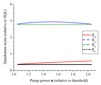
Figure 1: Prediction of the linearized theory for fluctuations in the sum/subtraction of field quadratures as a function of $\sigma$ for a shot noise limited pump beam. Full line: $S_{q+}$; dashed line: $S_{p+}$; line + crosses: $S_{p-}$; line + circles: $S_{q-}$

On the other hand, the sum of quadratures and pump fields’ subspaces are connected. This directly implies that excess noise in the pump beam degrades signal-idler entanglement, and can even destroy it optcomm04 . The behavior of the twin beams’ fluctuations as functions of pump power relative to threshold $\sigma$, for a shot noise limited pump, is presented in Fig. 1. The maximum squeezing of $S_{q+}$ occurs at threshold, and approaches shot noise for higher pump powers.

These behaviors change in the presence of excess noise in the pump. In this case, both $S_{q+}$ and $S_{p+}$ increase from their values at threshold. In particular, $S_{q+}$ goes from squeezing to excess noise. The point where it crosses the shot noise value solely depends on the amount of excess phase noise present in the pump beam. For this reason, it was necessary to filter the pump field in the experiment, in order to observe entanglement.

II.2 Noise spectra beyond the linearized model

We present here a comparison between the linearized approach to the quantum noise in the OPO and the numerical integration of the quantum stochastic equations in the positive P-representation. This will help us to eliminate the linearization procedure as the reason for the discrepancy between the theoretical prediction of squeezing and the experimentally observed excess phase noise for $\sigma>1.2$. We shall follow the procedure used in Ref. nos Although exact Heisenberg equations of motion can be found for this system, it is, at the very least, extremely difficult to solve nonlinear operator equations. We therefore develop stochastic equations of motion in the positive P-representation, which in principle give access to any normally-ordered operator expectation values we may wish to calculate. To find the appropriate equations, we proceed via the master and Fokker-Planck equations. Using the standard techniques for elimination of the baths hjc , we find the zero-temperature master equation for the reduced density operator. The master equation may be mapped onto a Fokker-Planck equation Crispin for the positive-P pseudoprobability distribution. The cavity damping rates at each frequency are $\gamma^{D}_{j}=2\gamma_{j}/\tau$, with $\gamma_{1}=\gamma_{2}=\gamma$. We further define $\gamma_{r}=\gamma_{0}/\gamma$. In order to apply perturbation theory, we introduce a normalized coupling constant,

$$g=\frac{\chi}{\gamma^{D}\sqrt{2\gamma_{r}}}\;,$$ (4)

which will be a power expansion parameter. Moreover, it will be useful to work with the scaled quadratures

$$x_{0}=g\sqrt{2\gamma_{r}}\,p_{0}\quad,\qquad q_{0}=g\sqrt{2\gamma_{r}}\,q_{0},$$

$$x_{+}=g\,p_{+}\quad,\;\qquad\qquad y_{+}=g\,q_{+},$$

$$x_{-}=g\,p_{-}\quad,\;\qquad\qquad y_{-}=g\,q_{-}\quad,$$ (5)

in order to render the stochastic equations amenable to perturbation. The stochastic equations for the scaled EPR variables become

$$\frac{dx_{0}}{dT} = -\gamma_{r}\left[x_{0}-2\sqrt{\sigma}+\frac{1}{2}\left(x_{+}^{2}-x_{-}^{2}-y_{+}^{2}+y_{-}^{2}\right)\right]\;,$$

$$\frac{dy_{0}}{dT} = -\gamma_{r}\left[y_{0}+x_{+}y_{+}-x_{-}y_{-}\right]\;,$$

$$\frac{dx_{-}}{dT} = -x_{-}-\frac{1}{2}\left[x_{0}x_{-}+y_{0}y_{-}\right]+\frac{g}{\sqrt{2}}\left[\sqrt{x_{0}+iy_{0}}\;\xi_{-}+\sqrt{x_{0}-iy_{0}}\;\xi_{-}^{+}\right]\;,$$ (6)

$$\frac{dy_{+}}{dT} = -y_{+}+\frac{1}{2}\left[y_{0}x_{+}-x_{0}y_{+}\right]-i\frac{g}{\sqrt{2}}\left[\sqrt{x_{0}+iy_{0}}\;\xi_{+}-\sqrt{x_{0}-iy_{0}}\;\xi_{+}^{+}\right]\;,$$

$$\frac{dx_{+}}{dT} = -x_{+}+\frac{1}{2}\left[x_{0}x_{+}+y_{0}y_{+}\right]+\frac{g}{\sqrt{2}}\left[\sqrt{x_{0}+iy_{0}}\;\xi_{+}+\sqrt{x_{0}-iy_{0}}\;\xi_{+}^{+}\right]\;,$$

$$\frac{dy_{-}}{dT} = -y_{-}+\frac{1}{2}\left[x_{0}y_{-}-y_{0}x_{-}\right]-i\frac{g}{\sqrt{2}}\left[\sqrt{x_{0}+iy_{0}}\;\xi_{-}-\sqrt{x_{0}-iy_{0}}\;\xi_{-}^{+}\right]\;,$$

where $T=\gamma^{D}\,t$ is time in units of the cavity lifetime for the down-converted fields. The functions $\xi_{\pm}(T)$ and $\xi_{\pm}^{+}(T)$ are independent Langevin forces with the following nonvanishing correlation functions:

$$\langle\xi_{+}(T)\xi_{+}(T^{\prime})\rangle = \langle\xi_{+}^{+}(T)\xi_{+}^{+}(T^{\prime})\rangle=\delta(T-T^{\prime})\;,$$

$$\langle\xi_{-}(T)\xi_{-}(T^{\prime})\rangle = \langle\xi_{-}^{+}(T)\xi_{-}^{+}(T^{\prime}T)\rangle=-\delta(T-T^{\prime})\;.$$ (7)

We notice the symmetry properties of the stochastic equations (6). In fact, it is easy to verify that the equations of motion are unchanged by the transformation $x_{-}\leftrightarrow y_{+}\,$ and $x_{+}\leftrightarrow-\,y_{-}\,$. Of course, all noise terms appearing in Eqs. (6) are statistically equivalent. Therefore, these equations should not change the symmetries of the initial values chosen for $x_{+}$ and $y_{-}$. In order to provide a comparison between the linearized model and the full stochastic integration, we will use a perturbation expansion of the positive P-representation of the dynamical equations. This allows us to include quantum effects in a systematic fashion ndturco . We first introduce a formal perturbation expansion in powers of the parameter $g$,

$$x_{k}=\sum_{n=0}^{\infty}g^{n}x_{k}^{(n)},$$

$$y_{k}=\sum_{n=0}^{\infty}g^{n}y_{k}^{(n)}.$$ (8)

The series expansion written in this way has the property that the zeroth order term corresponds to the classical field of order $1$ in the unscaled quadrature, while the first order term is related to quantum fluctuations of order $g$, and the higher order terms correspond to nonlinear corrections to the quantum fluctuations of order $g^{2}$ and greater. The stochastic equations are then solved by the technique of matching powers of $g$ in the corresponding time evolution equations. The steady state solutions $x_{js}$ of the zeroth order give the operation point of the OPO and describe its macroscopic behavior. For triply resonant operation, the expressions for the steady state are quite simple:

$$x_{0s} = 2\;,$$

$$x_{+s} = 2\,\left(\sqrt{\sigma}-1\right)^{1/2}\;,$$

$$x_{-s} = 0\;,$$ (9)

$$y_{0s} = y_{+s}=y_{-s}=0\;.$$

The first order equations are often used to predict squeezing in a linearized fluctuation analysis. They are non-classical in the sense that they can describe states without a positive-definite Glauber-Sudarshan P-distribution Roy ; Sudarshan , but correspond to a simple form of linear fluctuation which has a Gaussian quasi-probability distribution. A full quantum description of the OPO dynamics can be obtained by numerical integration of the stochastic equations (6), and can be compared to analytical expressions obtained from the linearized approach. Taking the first order terms and using the steady state solutions given by Eqs. (9), we can write the following equations for the linear quantum fluctuations,

$$\frac{dx_{0}^{(1)}}{dT} = -\gamma_{r}\left[x_{0}^{(1)}+2\,\left(\sqrt{\sigma}-1\right)^{1/2}x_{+}^{(1)}\right]\;,$$

$$\frac{dy_{0}^{(1)}}{dT} = -\gamma_{r}\left[y_{0}^{(1)}+2\,\left(\sqrt{\sigma}-1\right)^{1/2}y_{+}^{(1)}\right]\;,$$

$$\frac{dx_{+}^{(1)}}{dT} = -\left(\sqrt{\sigma}-1\right)^{1/2}\,x_{0}^{(1)}+\left(\xi_{+}+\xi_{+}^{+}\right)\;,$$ (10)

$$\frac{dx_{-}^{(1)}}{dT} = -2\,x_{-}^{(1)}+\left(\xi_{-}+\xi_{-}^{+}\right)\;,$$

$$\frac{dy_{+}^{(1)}}{dT} = -2\,y_{+}^{(1)}+\left(\sqrt{\sigma}-1\right)^{1/2}y_{0}^{(1)}-i\left(\xi_{+}-\xi_{+}^{+}\right)\;,$$

$$\frac{dy_{-}^{(1)}}{dT} = -i\left(\xi_{-}-\xi_{-}^{+}\right)\;.$$

The linear coupled stochastic equations obtained agree with Eqs. (3), for zero detunings and no spurious losses. From them, we may readily calculate the steady state averages of the first-order corrections and use that to compute the linearized fluctuations. Notice that under the linear approximation $y_{-}$ becomes a purely diffusive variable (phase diffusion). In an experimental situation, the noise spectra outside the cavity are generally the quantities of interest. We will therefore proceed to analyze the problem in frequency space, via Fourier decomposition of the fields. The first order stochastic equations may be rewritten in the frequency domain so that we may calculate the spectra of the squeezed and anti-squeezed field quadratures. The solutions for the noise of the squeezed operators, $\hat{p}_{-}$ and $\hat{q}_{+}$, are:

$$S_{p-}(\Omega^{\prime})=1-\frac{1}{\Omega^{\prime 2}+1}$$ (11)

and

$$S_{q+}(\Omega^{\prime})=1-\frac{(4\,\Omega^{\prime 2}+\gamma_{r}^{2})^{2}}{\Omega^{\prime 2}\left[4\,\Omega^{\prime 2}+\gamma_{r}^{2}-2\,\gamma_{r}\,\left(\sqrt{\sigma}-1\right)\right]^{2}+\left[4\,\Omega^{\prime 2}+\gamma_{r}^{2}\,\sqrt{\sigma}\right]^{2}}\;,$$ (12)

where $\Omega^{\prime}=\Omega/\gamma^{D}$ is the analysis frequency in units of the cavity bandwidth. Under the limits of the linearized approach, the results of the noise spectra are independent of the phase space representation employed. Therefore, these results coincide with the usual ones obtained with the Wigner representation. The spectra given by Eqs. (11) and (12) can now be compared with those found via stochastic integration of the full equations of motion (6) in the positive P-representation. The nonlinear spectra are calculated by Fourier transform of the stochastic integration, which must be performed numerically. A somewhat subtle point arises here: the nonlinear Eqs. (6) have more than one possible steady-state solution. Thus, for a fair comparison with the linearized spectra, it is necessary to choose the same steady-state. By doing this, we verified that both predictions, in the above-threshold OPO, agree within a good numerical precision. Therefore, we conclude that possible limitations of the linearized model for dealing with the OPO dynamics under phase diffusion do not account for the experimentally observed excess noise of $\hat{q}_{+}$.

III Experiment

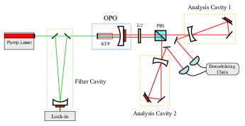
Figure 2: Sketch of the experimental setup.

Our system is a triply resonant type-II OPO operating above threshold. The experimental setup is depicted in Fig. 2. The pump beam is a diode-pumped doubled Nd:YAG laser (Innolight Diabolo) with 900 mW output power at 532 nm. A secondary output at 1064 nm is used for alignment purposes. Since the pump beam presents excess noise for frequencies as high as 20 MHz, a filter cavity is necessary. Our filter cavity has a bandwidth of 2.4 MHz and assures that the pump laser is shot noise limited for analysis frequencies higher than 15 MHz (see Fig. 3). We measured the laser phase noise by reflecting the beam off an empty cavity, in the same way we measure phase noise of the downconverted beams. The phase noise equals the intensity noise, except at a frequency of 12 MHz, where there is very big phase noise, owing to a frequency modulation inside the Diabolo laser, for stabilization purposes. This excess noise saturates our electronics and prevents measurements for analysis frequencies close to 12 MHz and also to its second harmonic, 24 MHz, as can be seen in Fig.  3. The OPO cavity is a linear semi-monolithic cavity composed of a flat input mirror, directly deposited on one face of the nonlinear crystal, with 93% reflectivity at 532 nm and high reflectivity ($>99.8$%) at 1064 nm, and a spherical output mirror (50 mm curvature radius) with high reflectivity at 532 nm ($>99.8$%) and 96% reflectivity at 1064 nm. The nonlinear crystal is a 10 mm-long Potassium Titanyl Phosphate (KTP) from Litton. Threshold power is 12 mW.

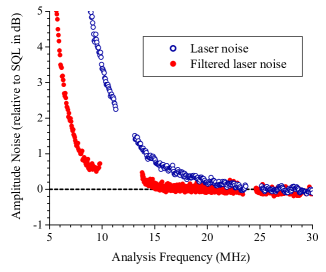
Figure 3: Measurement of the pump noise, as a function of the analysis frequency. Open circles: unfiltered laser noise; full circles: laser noise at the output of the filter cavity. In view of the large excess noise at 12 MHz and its second harmonic, we suppressed those frequencies from the data.

Signal and idler beams are separated by a polarizing beam splitter (PBS) and sent to detection, which consists of a ring cavity and a photodetector (Epitaxx ETX 300) for each beam. Overall detection efficiency is $\eta=80(2)\%$. Both analysis cavities have bandwidths of 14 MHz, allowing for a complete conversion of phase to amplitude noise for analysis frequencies higher than 20 MHz. Measurements are taken at analysis frequency equal to 27 MHz. In order to access the same quadrature for both beams, the two cavities must be detuned by the same amount at the same time. By scanning the detunings synchronously, we can measure all quadratures of the twin beams. In particular, we can easily select the amplitude (off resonance) or phase (detuning equal to half the bandwidth) quadraturesgalatola .

Data acquisition is carried out by a demodulating chain, which mixes the photocurrents from each detector with a sinusoidal electronic reference at the analysis frequency and filters the resulting low frequency signal. The demodulated photocurrent fluctuations are sampled at 600 kHz repetition rate by an A/D card connected to a personal computer. The variances of these fluctuations are then computed taking groups of 1000 points, resulting in something proportional to the photocurrents’ power spectrum at the analysis frequency. At the end, measured variances are normalized to the shot noise standard quantum level (SQL).

III.1 Fluctuations as a function of $\sigma$

The input pump field is guaranteed to be shot noise limited for frequencies above 15 MHz after being transmitted through the filter cavity. Even before being filtered, pump field is shot noise limited above 25 MHz, as shown in Fig. 3. Nevertheless, we observed excess noise in the sum of phases of signal and idler beams, preventing the violation of the inequality given in Eq. 1, except for pump powers very close to thresholdprlentangtwinopo .

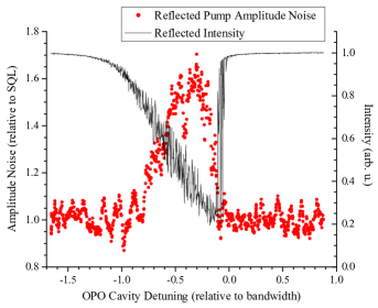
Figure 4: Intensity noise of the reflected pump beam, as a function of the detuning of the OPO cavity. The excess noise observed is peaked for $\Delta_{0}$ close to half the OPO cavity bandwidth. The asymmetry in the mean field signal is due to thermal bistability. The analysis frequency is 27 MHz. Circles: reflected pump noise; full line: reflected average intensity

As seen in section II, from the theoretical description of the OPO, excess noise in the pump beam would generate excess noise in the phase sum of the twin beams. Yet, how could that be the case if we carefully measured the input pump to be shot noise limited? By following this single lead, it is natural to examine the noise properties of the pump beam reflected from the OPO cavity. This was done by scanning the OPO cavity, for crystal temperatures such that there was no parametric oscillation (triple resonance depends sharply on crystal temperature and can be easily avoided). Since the incident beam is shot noise limited, could there be excess noise generated inside the cavity containing the KTP crystal? We did indeed find excess noise in the reflected pump’s amplitude (Fig. 4) and phase quadratures. The maximum values, for $\sigma=1$, were $S^{\mathrm{R}}_{p0}=1.8(1)$ and $S^{\mathrm{R}}_{q0}=4.5(3)$.

At present, we can still not claim to fully understand the origin of this excess noise. We verified, of course, that no such noise is generated in an empty cavity (which would also invalidate the measurements we perform with the analysis cavities for the twin beams). We also checked whether this effect depended on $\chi$ and would thus be directly related to the parametric process. For a polarization of the incident beam orthogonal to the usual polarization, phase matching can not be fulfilled, and no downconversion can occur. The noise in the reflected beam did not show any significant dependence on the incident polarization. It does, however, increase for increasing power of the incident beam. We can speculate that this can be a result of photon absorption by the crystal at 532 nm (which is at the origin of the thermal bistability observed in Fig. 4), with subsequent relaxation by spontaneous emission or non-radiative processes. This may give rise to an intensity-dependent refractive index, yielding phase and amplitude modulation at 532 nm. We are currently investigating these possibilities.

As a first approximation, in order to see whether this would account for the behavior of $\Delta^{2}\hat{p}_{-}$, $\Delta^{2}\hat{q}_{-}$, $\Delta^{2}\hat{p}_{+}$, and $\Delta^{2}\hat{q}_{+}$, as a function of $\sigma$, we simply added excess noise to the input pump beam in the linearized OPO theory. In Fig. 5, we compare the results from the model, with incident $S_{p0}=1.5$ and $S_{q0}=5.5$, to the measured data. Signal and idler powers varied from 0.4mW up to 5.5mW each during the experiment, corresponding to pump powers between 13mW and 26mW, or $1.06<\sigma<2.2$. As expected, noises corresponding to the subtraction subspace, $\Delta^{2}\hat{p}_{-}$ and $\Delta^{2}\hat{q}_{-}$, are independent of pump power. But $\Delta^{2}\hat{q}_{+}$ is very sensitive to $\sigma$, as well as $\Delta^{2}\hat{p}_{+}$ to a smaller degree. The agreement with the theoretical model is surprisingly good. This is a strong indication that the intracavity pump excess noise is the main responsible for the excess noise in $\Delta^{2}\hat{q}_{+}$.

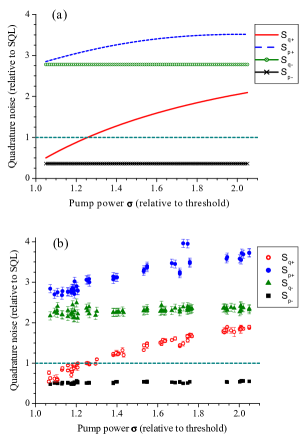
Figure 5: Noise behavior as a function of $\sigma$. In part (a), we present the predictions of the linearized model, for an input pump beam with $S_{p0}=1.5$ and $S_{q0}=5.5$; dashed line: $S_{p+}$; full line + open circles: $S_{q-}$; full line: $S_{q+}$; full line + crosses: $S_{p-}$; SQL = 1.0 is indicated by a dashed line. In part (b), experimental results are shown for $\sigma$ ranging from 1.06 to 2.2. full circles: $S_{p+}$; triangles: $S_{q-}$; open circles: $S_{q+}$; squares: $S_{p-}$; SQL = 1.0 is indicated by a dashed line.

III.2 Two-color entanglement

The sum of phases’ noise is squeezed very close to threshold, and squeezing is degraded with increasing pump power. $\Delta^{2}\hat{q}_{+}$ crosses the shot noise level approximately at $\sigma=1.20$, from squeezing to anti-squeezing, although only below $\sigma=1.15$ can squeezing be observed with certainty.

Fig. 6 shows the recorded noise in sum and subtraction of photocurrent fluctuations of signal and idler beams as functions of analysis cavities’ detuning, for $\sigma=1.06$. Off resonance, quantum correlations are observed in the subtraction of amplitudes, $\Delta^{2}\hat{p}_{-}=0.50(1)$, or $-3.01(9)$ dB. For analysis cavities’ detuning equal to half the bandwidth, squeezing is present in the sum of phases, $\Delta^{2}\hat{q}_{+}=0.73(1)$, or $-1.37(6)$ dB. The Duan et al. and Simon criterion, Eq.(1), is then clearly violated,

$$\Delta^{2}\hat{p}_{-}+\Delta^{2}\hat{q}_{+}=1.23(2)<2\;,$$ (13)

attesting the entanglement. This value, together with the one reported by Jing et al.pfisterentang , is the lowest achieved for twin beams produced by an above-threshold OPO.

Figure 6: Sum (full circles) and difference (open circles) of quadratures’ noise, measured as a function of the analysis cavities’ detuning. Squeezed-state entanglement can be directly observed, with $\Delta^{2}\hat{p}_{-}=0.50(1)$, or $-3.01(9)$ dB, and $\Delta^{2}\hat{q}_{+}=0.73(1)$, or $-1.37(6)$ dB

We also point out that, in this experiment, the twin beams have very different frequencies (wavelengths differ by $\approx 1$ nm), an unusual situation. Such two-color entanglement can be very interesting for the transfer of quantum information between different parts of the electromagnetic spectrum.

IV Conclusion

We presented a theoretical and experimental investigation of phase noise and entanglement in the above-threshold OPO. Excess noise in the phase sum of the twin beams was measured as a function of pump power relative to threshold and we found that it decreases as pump power is lowered. We finally discovered that excess pump noise is generated inside the OPO cavity containing the nonlinear crystal, even for a shot noise limited pump beam and without parametric oscillation. The ultimate physical origin of this phenomenon still requires further investigation. Another important question to address is how one can eliminate this effect. Su et al.optlettpeng were able to observe entanglement for $\sigma$ of the order of two. The difference between their setup and others is a lower cavity finesse for the pump field. If the assumption of an intensity dependent index of refraction is correct, this makes sense. For a lower finesse, phase shifts accumulated inside the cavity should be smaller, hence the excess noise generated should also be smaller.

In spite of these unexpected phenomena, two-color entanglement was measured in the above-threshold OPO. There are interesting avenues to pursue for applications in quantum information. First of all, we should mention that the strongest squeezing measured to date, $-9.7$ dB, was generated in an above-threshold OPOclaude10db . Thus, entanglement in the above-threshold OPO may be the strongest ever achieved for continuous variables. The bright twin beams can have very different frequencies, and one can envisage CV quantum teleportationkimbleteleport to transfer quantum information from one frequency to another (in other words, to “tune” quantum information). For example, this system could be used to communicate quantum information between quantum memories or quantum computers based on “hardwares” which have different resonance frequencies. Finally, a quantum key distribution protocol proposed by Silberhorn et al.qkdleuchs can be readily implemented, with the advantage that the measurement with analysis cavities does not require sending a local oscillator together with the quantum channel to the distant receiver.

The above-threshold OPO, which was the first system proposed to observe continuous variable entanglement, has finally been added to the optical quantum information toolbox. We expect new and exciting applications to come in the near future.

References

- (1) R. H. Kingston, “Parametric amplification and oscillation of optical frequencies”, Proc. IRE 50, 472–474 (1962).
- (2) R. Graham and H. Haken, “The quantum fluctuations of the optical parametric oscillator,” Z. Phys. 210, 276–302 (1968).
- (3) L.-A. Wu, H. J. Kimble, J. L. Hall, and H. Wu, “Generation of Squeezed States by Parametric Down Conversion”, Phys. Rev. Lett. 57, 2520–2523 (1986).
- (4) A. Heidmann, R. J. Horowicz, S. Reynaud, E. Giacobino, C. Fabre, and G. Camy, “Observation of Quantum Noise Reduction on Twin Laser Beams”, Phys. Rev. Lett. 59, 2555–2557 (1987).
- (5) M. D. Reid and P. D. Drummond, “Quantum Correlations of Phase in Nondegenerate Parametric Oscillation”, Phys. Rev. Lett. 60, 2731–2733 (1988).
- (6) Z. Y. Ou, S. F. Pereira, H. J. Kimble, and K. C. Peng, “Realization of the Einstein-Podolsky-Rosen Paradox for Continuous Variables”, Phys. Rev. Lett. 68, 3663–3666 (1992).
- (7) S. L. Braunstein and P. van Loock, “Quantum information with continuous variables”, Rev. Mod. Phys. 77, 513–577 (2005).
- (8) W. P. Bowen, R. Schnabel, P. K. Lam, and T. C. Ralph, “Experimental Investigation of Criteria for Continuous Variable Entanglement”, Phys. Rev. Lett. 90, 043601 (2003).
- (9) C. Schori, J. L. Sorensen, and E. S. Polzik, “Narrow-band frequency tunable light source of continuous quadrature entanglement”, Phys. Rev. A 66, 033802 (2002).
- (10) A. Furusawa, J. L. Sorensen, S. L. Braunstein, C. A. Fuchs, H. J. Kimble, and E. S. Polzik, “Unconditional Quantum Teleportation”, Science 282, 706–709 (1998).
- (11) X. J. Jia, X. L. Su, Q. Pan, J. G. Gao, C. D. Xie, and K. C. Peng, “Experimental Demonstration of Unconditional Entanglement Swapping for Continuous Variables”, Phys. Rev. Lett. 93, 250503 (2004).
- (12) A. S. Villar, L. S. Cruz, K. N. Cassemiro, M. Martinelli, and P. Nussenzveig, “Generation of Bright Two-Color Continuous Variable Entanglement”, Phys. Rev. Lett. 95 243603 (2005).
- (13) X. L. Su, A. Tan, X. J. Jia, Q. Pan, C. D. Xie, and K. C. Peng, “Experimental demonstration of quantum entanglement between frequency-nondegenerate optical twin beams”, Opt. Lett. 31, 1133–1135 (2006).
- (14) J. Jing, S. Feng, R. Bloomer, and O. Pfister, “Experimental continuous-variable entanglement of phase-locked bright optical beams”, e-print arXiv:quant-ph/0604134.
- (15) Lu-Ming Duan, G. Giedke, J. I. Cirac, and P. Zoller, “Inseparability Criterion for Continuous Variable Systems”, Phys. Rev. Lett. 84, 2722–2725 (2000).
- (16) R. Simon, “Peres-Horodecki Separability Criterion for Continuous Variable Systems”, Phys. Rev. Lett. 84, 2726–2729 (2000).
- (17) A. S. Villar, M. Martinelli, and P. Nussenzveig, “Testing the entanglement of intense beams produced by a non-degenerate Optical Parametric Oscillator”, Opt. Commun. 242, 551–563 (2004).
- (18) J. Laurat, L. Longchambon, C. Fabre, and T. Coudreau, “Experimental investigation of amplitude and phase quantum correlations in a type II optical parametric oscillator above threshold: from nondegenerate to degenerate operation”, Opt. Lett. 30, 1177–1179 (2005).
- (19) M. D. Reid and P. D. Drummond, “Correlations in nondegenerate parametric oscillation - squeezing in the presence of phase diffusion”, Phys. Rev. A40, 4493–4506 (1989).
- (20) P. D. Drummond and M. D. Reid, “Correlations in nondegenerate parametric oscillation. 2. Below threshold results”, Phys. Rev. A41, 3930–3949 (1990).
- (21) S. Chaturvedi, P. D. Drummond and D. F. Walls, “2 Photon absorption with coherent and partially coherent driving fields ”, J. Phys. A 10, L187–L192 (1977).
- (22) P. D. Drummond and C. W. Gardiner, “Generalized P-Representations in quantum optics”, J. Phys. A 13, 2353–2368 (1980).
- (23) K. V. Kheruntsyan and K. G. Petrosyan, “Exact steady-state Wigner function for a nondegenerate parametric oscillator”, Phys. Rev. A62, 015801 (2000).
- (24) B. Coutinho dos Santos, K. Dechoum, A. Z. Khoury, L. F. da Silva, and M. K. Olsen, “Quantum analysis of the nondegenerate optical parametric oscillator with injected signal”, Phys. Rev. A72, 033820, (2005).
- (25) H. J. Carmichael, Statistical Methods in Quantum Optics 1: Master Equations and Fokker-Planck Equations, (Springer, Berlin, 1999).
- (26) C. W. Gardiner, Quantum Noise, Springer-Verlag, Berlin, (1991).
- (27) K. Dechoum, P. D. Drummond, S. Chaturvedi, and M. D. Reid, “Critical fluctuations and entanglement in the nondegenerate parametric oscillator” Phys. Rev. A70, 053807 (2004).
- (28) R. J. Glauber, “Coherent and incoherent states of the radiation field” Phys. Rev. 131, 2766–2788 (1963).
- (29) E. C. G. Sudarshan, “Equivalence of Semiclassical and Quantum Mechanical Descriptions of Statistical Light Beams”, Phys. Rev. Lett. 10, 277–279 (1963).
- (30) P. Galatola, L. A. Lugiato, M. G. Porreca, P. Tombesi, and G. Leuchs, “System control by variation of the squeezing phase”, Opt. Commun. 85, 95–103 (1991).
- (31) Ch. Silberhorn, N. Korolkova, and G. Leuchs, “Quantum Key Distribution with Bright Entangled Beams”, Phys. Rev. Lett. 88, 167902 (2002).