Information-Disturbance Tradeoff in Quantum State Discrimination

Abstract

When discriminating between two pure quantum states, there exists a quantitative tradeoff between the information retrieved by the measurement and the disturbance caused on the unknown state. We derive the optimal tradeoff and provide the corresponding quantum measurement. Such an optimal measurement smoothly interpolates between the two limiting cases of maximal information extraction and no measurement at all.

I Introduction

The problem of discriminating between two different quantum states reveals two main features that make Quantum Theory so much different from the classical intuition. First, quantum state discrimination involves in-principle indistinguishability of quantum states: it is well known that it is not possible to perfectly infer (by means of a one-shot experiment) which state we eventually picked at random from a set of non orthogonal quantum states. Of course, it is nonetheless possible to perform such a decision in an optimal way, e. g., by minimizing the error probability of discrimination helstrom , by a minimax strategy where the smallest of the probabilities of correct detection is maximized mmax , or looking for optimal unambiguous discrimination unambiguous , where unambiguity is paid by the possibility of getting inconclusive results from the measurement. Second, quantum indistinguishability principle is closely related to another very popular—yet often misunderstood—principle (formerly known as Heisenberg principle heisenberg ; fuco ; banaszek01.prl ): it is not possible to extract information from a quantum system without perturbing it somehow. In fact, if the experimenter could gather information about an unknown quantum state without disturbing it at all, even if such information is partial, by performing further non-disturbing measurements on the same system, he could finally determine the state, in contradiction with the indistinguishability principle gdm-yuen .

Actually, there exists a precise tradeoff between the amount of information extracted from a quantum measurement and the amount of disturbance caused on the system, analogous to Heisenberg relations holding in the preparation procedure of a quantum state. Quantitative derivations of such a tradeoff have been obtained in the scenario of quantum state estimation hol ; qse . The optimal tradeoff has been derived in the following cases: in estimating a single copy of an unknown pure state banaszek01.prl , many copies of identically prepared pure qubits banaszek01.pra and qudits mf , a single copy of a pure state generated by independent phase-shifts mista05.pra , an unknown maximally entangled state max , an unknown coherent state cv and Gaussian state paris . Experiment realization of minimal disturbance measurements has been also reported dema ; cv .

The present paper aims at fully characterize such a tradeoff relation in quantum state discrimination, in the case in which the unknown quantum state is chosen with equal a priori probability from a set of two non orthogonal pure states, and the error probability of the discrimination is allowed to be suboptimal (thus intuitively causing less disturbance with respect to the optimal discrimination). We explicitly provide a measuring strategy—both in terms of outcome probabilities and state-reduction—that achieves the optimal tradeoff, which smoothly interpolates between the two limiting cases of maximal information extraction and no measurement at all. As a byproduct, we also recover in a simpler way some of the results of Ref. fuco . Our explicit derivation of the quantum measurement should allow to carry out a feasibility study for the experimental realization of minimal-disturbing measurements. The issue of the information-disturbance tradeoff for state discrimination can become of practical relevance for posing general limits in information eavesdropping and for analyzing security of quantum cryptographic communications.

The paper is organized as follows. In Sec. II, we briefly review the problem of minimum-error state discrimination, and obtain the minimum disturbance for the minimum-error measurement. In Sec. III, we provide the general solution of the optimal information-disturbance tradeoff, along with the corresponding measurement instrument. In Sec. IV, we suggest an experimental realization of the minimum-disturbing measurement and conclude the paper with closing remarks.

II Minimum disturbance for minimum-error state discrimination

Typically, in quantum state discrimination we are given two (fixed) non orthogonal pure states $\psi_{1}$ and $\psi_{2}$, with a priori probabilities $p_{1}$ and $p_{2}=1-p_{1}$, and we want to construct a measurement discriminating between the two. In the following, in order to work in full generality, we will describe a measurement by means of the quantum instruments formalism davies-lewis , namely, a collection of completely positive maps $\{\mathcal{E}_{i}\}$, labelled by the measurement outcomes $\{i\}$. By exploiting the well known Kraus decomposition kraus , one can always write $\mathcal{E}_{i}(\rho)=\sum_{k}E^{(i)}_{k}\rho E^{(i){\dagger}}_{k}$. In the case the sum comprises just one term, namely, $\mathcal{E}_{i}(\rho)=E_{i}\rho E^{\dagger}_{i}$, the map $\mathcal{E}_{i}$ is called pure, since it maps pure states into pure states. The trace $\operatorname{Tr}[\mathcal{E}_{i}(\rho)]=\operatorname{Tr}[\Pi_{i}\rho]$, where $\Pi_{i}=\sum_{k}E^{(i){\dagger}}_{k}E^{(i)}_{k}$ is a positive operator associated to the $i$-th outcome, provides the probability that the measurement performed on a quantum system described by the density matrix $\rho$ gives the $i$-th outcome. The posterior (or reduced) state after the measurement is given by $\rho_{i}=\mathcal{E}_{i}(\rho)/\operatorname{Tr}[\mathcal{E}_{i}(\rho)]$. The averaged reduced state—coming from ignoring the measurement outcome—is simply obtained using the trace-preserving map $\mathcal{E}=\sum_{i}\mathcal{E}_{i}$. The trace-preservation constraint for $\mathcal{E}$ implies that the set of positive operators $\{\Pi_{i}\}$ is actually a positive operator-valued measure (POVM), satisfying the completeness condition $\sum_{i}\Pi_{i}=\openone$.

Quantum state discrimination is then performed by a two-outcome instrument $\{\mathcal{E}_{1},\mathcal{E}_{2}\}$ whose capability of discriminating between $\psi_{1}$ and $\psi_{2}$ can be evaluated by the average success probability

$$\begin{split}P(\{\mathcal{E}_{1},\mathcal{E}_{2}\})&=\sum_{i=1}^{2}p_{i}\operatorname{Tr}[\mathcal{E}_{i}(|\psi_{i}\rangle\langle\psi_{i}|)]\\ &=\sum_{i=1}^{2}p_{i}\operatorname{Tr}[\Pi_{i}|\psi_{i}\rangle\langle\psi_{i}|].\end{split}$$ (1)

Notice that $P$ actually depends only on the POVM $\{\Pi_{i}\}$. The probability $P$ quantifies the amount of information that the instrument $\{\mathcal{E}_{1},\mathcal{E}_{2}\}$ is able to extract from the ensemble $\{p_{1},\psi_{1};p_{2},\psi_{2}\}$. Among all instruments achieving average success probability $\bar{P}$ (the bar over $P$ means that we fix the value of $P$), we are interested in those minimizing the average disturbance caused on the unknown state, that we evaluate in terms of average fidelity, namely,

$$D(\{\mathcal{E}_{1},\mathcal{E}_{2}\},\bar{P})=1-\sum_{i=1}^{2}p_{i}\langle\psi_{i}|\mathcal{E}(|\psi_{i}\rangle\langle\psi_{i}|)|\psi_{i}\rangle.$$ (2)

Differently from $P$, the disturbance $D$ strongly depends on the particular form of the instrument $\{\mathcal{E}_{i}\}$. This means that there exist many different instruments achieving the same $P$, but giving different values of $D$. Let

$$\bar{D}(\bar{P})=\min_{\{\mathcal{E}_{1},\mathcal{E}_{2}\}}D(\{\mathcal{E}_{1},\mathcal{E}_{2}\},\bar{P})$$ (3)

be the disturbance produced by the least disturbing instrument that discriminates $\psi_{1}$ from $\psi_{2}$ with average success probability $\bar{P}$. Intuitive arguments suggest that the larger is $\bar{P}$, the larger must correspondingly be $\bar{D}$ (i. e., the larger is the amount of information extracted, the larger is the disturbance caused by the measurement). Our aim is to quantitatively derive such a tradeoff, along with the corresponding measurement instrument. From now on we will restrict to the case of equal a priori probabilities, i. e. $p_{1}=p_{2}=1/2$.

Let us start reviewing the case of the measurement maximizing $P$. First of all notice that, given two generally non orthogonal pure states $\psi_{1}$ and $\psi_{2}$, it is always possible to choose an orthonormal basis $\{|1\rangle,|2\rangle\}$, placed symmetrically around $\psi_{1}$ and $\psi_{2}$ (see Fig. 1), on which both states have real components, namely

$$\begin{split}&|\psi_{1}\rangle=\cos\alpha\;|1\rangle+\sin\alpha\;|2\rangle,\\ &|\psi_{2}\rangle=\sin\alpha\;|1\rangle+\cos\alpha\;|2\rangle,\end{split}$$ (4)

and fidelity $f=|\langle\psi_{1}|\psi_{2}\rangle|=\sin 2\alpha$. In this case, it is known helstrom that the maximum achievable $P$ is

$$P_{\textrm{opt}}=\cos^{2}\alpha,$$ (5)

which is obtained by the orthogonal von Neumann measurement $\{|1\rangle\langle 1|,|2\rangle\langle 2|\}$.

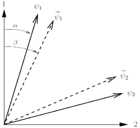
Figure 1: Helstrom’s scheme to optimally discriminate between to non orthogonal states $\psi_{1}$ and $\psi_{2}$. The orthogonal axes $1$ and $2$ correspond to the von Neumann measurement that achieves the optimal discrimination probability (5). According to the measurement outcome, $\widetilde{\psi}_{1}$ and $\widetilde{\psi}_{2}$ are the states to be prepared, in order to minimize the disturbance, see Eq. (9).

Which is the instrument, among all instruments achieving $P_{\textrm{opt}}$, that minimizes the disturbance $D$? Let us assume for the moment (the optimality of this assumption will be proved in full generality in the second part of the paper) that such an instrument is pure. Intuitively, this means that we are excluding a classical shuffling of outcomes. Then, since $P_{\textrm{opt}}$ is reached by a rank-one von Neumann measurement, we can write

$$\mathcal{E}_{i}(\rho)=U_{i}|i\rangle\langle i|\rho|i\rangle\langle i|U^{\dagger}_{i},\qquad i=1,2,$$ (6)

where $U_{i}$ is a unitary operator. Letting $U_{i}|i\rangle=|\widetilde{\psi}_{i}\rangle$, one recognizes in Eq. (6) a measure-and-prepare realization: the observable $|i\rangle\langle i|$ is measured and, depending on the outcome, the quantum state $\widetilde{\psi}_{i}$ is prepared, i. e. one has $\mathcal{E}_{i}(\rho)=|\widetilde{\psi}_{i}\rangle\langle\widetilde{\psi}_{i}|\operatorname{Tr}[\rho|i\rangle\langle i|]$. By symmetry arguments (under the label exchange “$1$” $\leftrightarrow$ “$2$”), $U_{1}=U_{2}^{\dagger}$, namely, the $\widetilde{\psi}_{i}$’s are symmetrically tilted with respect to the $\psi_{i}$’s, see Fig. 1. With this notation, $D$ can be rewritten as

$$D(P_{\textrm{opt}})=1-\frac{1}{2}\sum_{i,j=1}^{2}|\langle j|\psi_{i}\rangle|^{2}|\langle\psi_{i}|\widetilde{\psi}_{j}\rangle|^{2}.$$ (7)

Since $|\langle i|\psi_{i}\rangle|^{2}=\cos^{2}\alpha$, $|\langle\psi_{i}|\widetilde{\psi}_{i}\rangle|^{2}=\cos^{2}(\beta-\alpha)$, and, for $i\neq j$, $|\langle j|\psi_{i}\rangle|^{2}=\sin^{2}\alpha$, and $|\langle\psi_{i}|\widetilde{\psi}_{j}\rangle|^{2}=\sin^{2}(\alpha+\beta)$, minimizing the disturbance (7) resorts to minimizing the following function $D(\beta)$ of the tilt $\beta$

$$D(\beta)=1-\cos^{2}\alpha\cos^{2}(\beta-\alpha)-\sin^{2}\alpha\sin^{2}(\alpha+\beta),$$ (8)

where $\alpha$ is a parameter, fixed along with the input states. Solving the equation $\operatorname{d}D(\beta)/\operatorname{d}\beta=0$, it turns out that the tilt $\beta$ minimizing the disturbance is related to the angle $\alpha$ by

$$\tan 2\beta=\frac{\tan 2\alpha}{\cos 2\alpha},$$ (9)

in agreement with Ref. fuco . From the above equation, $\beta\geq\alpha$. The presence of the tilt $\beta$ can be geometrically explained starting from the observation that, for non orthogonal states, minimum error discrimination can never be error-free. In other words, even using the optimal Helstrom’s measurement, there is always a non zero error probability, and, the closer the input states are to each other, the smaller the success probability is. Hence it is reasonable that, the closer the input states are, the less “trustworthy” the measurement outcome is, and the average disturbance is minimized by cautiously preparing a new state that actually is a coherent superpositions of both hypotheses $\psi_{1}$ and $\psi_{2}$. Using Eq. (9), from Eq. (8) one obtains the minimum disturbance for Helstrom’s optimal measurement

$$D_{\textrm{opt}}=\frac{4-\sqrt{14+2\cos 8\alpha}}{8}.$$ (10)

Notice that $D_{\textrm{opt}}$ reaches its maximum for $\alpha=\pi/8$, namely, when $\psi_{1}$ and $\psi_{2}$ are “unbiased” with respect to each other ($|\langle\psi_{1}|\psi_{2}\rangle|^{2}=1/2$).

III The general solution

We analysed the limiting case in which the information extraction is maximized—i. e. the average success probability is maximized. The opposite limiting case is when we do not perform any measurement at all, without disturbing the states. The main result of the paper is to provide the optimal tradeoff for all intermediate situations, along with the corresponding quantum instrument. In order to do this, it is useful to exploit the Choi-Jamiołkowski isomorphism choi-jam between completely positive maps $\mathcal{M}$ on states on $\mathcal{H}$ and positive operators $R_{\mathcal{M}}$ on $\mathcal{H}\otimes\mathcal{H}$

$$\mathcal{M}\longleftrightarrow R_{\mathcal{M}}=(\mathcal{M}\otimes\mathcal{I})|\Omega\rangle\langle\Omega|$$ (11)

where $|\Omega\rangle=\sum_{k=1}^{d}|k\rangle\otimes|k\rangle$ is the (non normalized) maximally entangled vector in the $d^{2}$-dimensional Hilbert space $\mathcal{H}\otimes\mathcal{H}$ (in our case, $\mathcal{H}$ is two-dimensional). The correspondence (11) is one-to-one, the inverse formula being

$$\mathcal{M}(\rho)=\operatorname{Tr}_{2}[(\openone\otimes\rho^{*})\ R_{\mathcal{M}}],$$ (12)

where $\operatorname{Tr}_{2}$ denotes the trace over the second Hilbert space, and $\rho^{*}$ is the complex conjugated of $\rho$, with respect to the basis fixed by $|\Omega\rangle$ in Eq. (11). In terms of Choi-Jamiołkowski operator, trace-preservation condition is given by $\operatorname{Tr}_{1}[R_{\mathcal{M}}]=\openone$.

An instrument $\{\mathcal{E}_{1},\mathcal{E}_{2}\}$ can then be put in correspondence with a set of positive operators $\{R_{1},R_{2}\}$. Clearly, $0<\operatorname{Tr}_{1}[R_{1}]<\openone$ and $0<\operatorname{Tr}_{1}[R_{2}]<\openone$, while $\operatorname{Tr}_{1}[R_{1}+R_{2}]=\openone$, since the total operator $R=R_{1}+R_{2}$ corresponds to the trace-preserving map $\mathcal{E}=\mathcal{E}_{1}+\mathcal{E}_{2}$. The average success probability (1) and the average disturbance (2) can be rewritten as

$$P=\frac{1}{2}\sum_{i=1}^{2}\operatorname{Tr}[(\openone\otimes|\psi_{i}\rangle\langle\psi_{i}|^{*})\ R_{i}],$$ (13)

$$D=1-\frac{1}{2}\sum_{i=1}^{2}\operatorname{Tr}[(|\psi_{i}\rangle\langle\psi_{i}|\otimes|\psi_{i}\rangle\langle\psi_{i}|^{*})\ R],$$ (14)

respectively. (In the following, we will drop the star, since $\psi_{1}$ and $\psi_{2}$ have real components over the basis $\{|1\rangle,|2\rangle\}$.) Our strategy is to fix the average success probability $1/2\leq P_{t}\leq P_{\textrm{opt}}$ by fixing the value of a control parameter $t$, i. e.

$$P_{t}=tP_{\textrm{opt}}+\frac{1-t}{2}=t\cos^{2}\alpha+\frac{1-t}{2},$$ (15)

with $0\leq t\leq 1$, and then to search, among all possible measurements achieving $P_{t}$, for the one minimizing the disturbance $D(P_{t})$. In the symmetric case, $p_{1}=p_{2}=1/2$, the minimization problem can be strikingly simplified by exploiting the exchange symmetry $|\psi_{1}\rangle=\sigma_{x}|\psi_{2}\rangle$, where $\sigma_{x}=\begin{pmatrix}0&1\\ 1&0\end{pmatrix}$, in the $\{|1\rangle,|2\rangle\}$ basis. It is then simple to check that, given an instrument $\{R_{1},R_{2}\}$ achieving average success probability $P$ and disturbance $D$, the instrument $\{R^{\prime}_{1},R^{\prime}_{2}\}$ constructed as

$$R^{\prime}_{i}=\frac{1}{2}(R_{i}+\sigma_{x}^{\otimes 2}R_{j}\sigma_{x}^{\otimes 2}),\qquad i\neq j,$$ (16)

achieves the same values of $P$ and $D$ as well. Hence, without loss of generality, we can restrict ourselves to instruments satisfying $R_{2}=\sigma_{x}^{\otimes 2}R_{1}\sigma_{x}^{\otimes 2}$. Then, the average disturbance (14) can be rewritten as $D=1-\operatorname{Tr}[\Sigma\ R_{1}]$, where $\Sigma=\sum_{i}|\psi_{i}\rangle\langle\psi_{i}|^{\otimes 2}$, and the optimization problem (3) over a two-outcome instrument resorts to the following—much simpler—optimization over a single positive operator $R_{1}$

$$D_{t}=\min_{\{\mathcal{E}_{1},\mathcal{E}_{2}\}}D(P_{t})=1-\max_{R_{1}}\operatorname{Tr}[\Sigma\ R_{1}],$$ (17)

with the trace-preservation constraint $\operatorname{Tr}_{1}[R_{1}+\sigma_{x}^{\otimes 2}R_{1}\sigma_{x}^{\otimes 2}]=\openone$, and the constraint of average success probability equal to $P_{t}$, namely $\operatorname{Tr}[(\openone\otimes|\psi_{1}\rangle\langle\psi_{1}|)\ R_{1}]=P_{t}$. These constraints can be recast as four linear conditions:

$$R_{1}\geq 0,\quad \operatorname{Tr}[R_{1}]=1,$$

$$\operatorname{Tr}[(\openone\otimes\sigma_{x})\ R_{1}]=0,\quad \operatorname{Tr}[(\openone\otimes\sigma_{z})\ R_{1}]=\frac{2P_{t}-1}{\cos 2\alpha},$$

where $\sigma_{z}=\begin{pmatrix}1&0\\ 0&-1\end{pmatrix}$. Basic linear programming methods, along with the reconstruction formula (12), show that, for every value of $P_{t}$, the minimum disturbance $D_{t}$ is achieved by the pure instrument $\mathcal{E}_{i}^{(t)}(\rho)=E_{i}^{(t)}\rho E_{i}^{(t){\dagger}}$, where

$$\begin{split}E_{1}^{(t)}&=U(t)\left(\frac{\sqrt{1-\gamma}}{2}\sigma_{z}+\frac{\sqrt{1+\gamma}}{2}\openone\right),\\ E_{2}^{(t)}&=U^{\dagger}(t)\left(-\frac{\sqrt{1-\gamma}}{2}\sigma_{z}+\frac{\sqrt{1+\gamma}}{2}\openone\right),\end{split}$$ (19)

with $\gamma=\sqrt{1-t^{2}}$. The unitary operator $U(t)$ in the above equation generalizes that in Eq. (6) as follows

$$U(t)=\begin{pmatrix}\cos\beta_{t}&\sin\beta_{t}\\ -\sin\beta_{t}&\cos\beta_{t}\end{pmatrix},$$ (20)

where notafuco

$$\tan 2\beta_{t}=\frac{t\sin 2\alpha}{\cos^{2}2\alpha+\gamma\sin^{2}2\alpha}.$$ (21)

It follows that every instrument that achieves average success probability $P_{t}$ must cause at least an average disturbance

$$\begin{split}D_{t}&=\frac{1}{2}\left(1-t\sin 2\alpha\sin 2\beta_{t}\right)\\ &+\frac{\cos 2\beta_{t}}{4}\left[\gamma(\cos 4\alpha-1)-\cos 4\alpha-1\right].\end{split}$$ (22)

It is also simple to check that

$$\Pi_{i}^{(t)}=E_{i}^{(t){\dagger}}E_{i}^{(t)}=t|i\rangle\langle i|+\frac{1-t}{2}\openone,$$ (23)

namely, the POVM of the measurement is the convex mixture of the optimal one $\{|1\rangle\langle 1|,|2\rangle\langle 2|\}$ and a completely random one. On the contrary, the instrument operators (19) represents a coherent superposition of Helstrom’s (see Eq. (6)) and the identity map.

Just by varying the control parameter $t$, it is possible to smoothly move between the limiting cases. For $t=0$, we obtain the identity map, that is, the no-measurement case. For $t=1$, we obtain Helstrom’s instrument in Eq. (6), thus proving that assuming pure instruments is in fact the optimal choice. In particular, Eq. (21) provides the tilt given in Eq. (9). However, the crucial difference between Helstrom’s limit ($t=1$) and the intermediate cases is that, for $t<1$, the optimal instrument cannot be interpreted by means of a measure-and-prepare scheme, and the unitaries $U(t)$ and $U^{\dagger}(t)$ in Eq. (19) represent feedback rotations for outcomes $1$ and $2$.

By eliminating the parameter $t$ from Eqs. (15) and (22), we obtain the optimal tradeoff $D(P)$ between information and disturbance, for any value of $\alpha$, namely for any couple of states with fidelity $f=\sin 2\alpha$. We plot $D(P)$ in Fig. 2, for three different values of $f$, i.e. $f^{2}=\frac{3}{4},\frac{1}{2},\frac{1}{4}$.

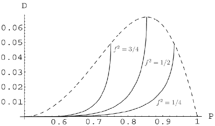
Figure 2: Optimal tradeoff between disturbance and discrimination probability of two pure states $\psi_{1}$ and $\psi_{2}$ for three different values of the fidelity $f=|\langle\psi_{1}|\psi_{2}\rangle|$, i.e. $f^{2}=\frac{3}{4},\frac{1}{2},\frac{1}{4}$. The convolution of ending points (the dashed curve) provides the minimal disturbance for Helstrom’s optimal measurement, namely $D_{\textrm{opt}}$ of Eq. (10), with $P=\cos^{2}\alpha$.

The expression of $D(P)$ is rather involved, however it can be simplified upon introducing the renormalized quantities $\mathscr{I}$ and $\mathscr{D}$ as follows

$$\mathscr{I}=\frac{P-1/2}{P_{\textrm{opt}}-1/2},\qquad\mathscr{D}=\frac{D}{D_{\textrm{opt}}},$$ (24)

where $P_{\textrm{opt}}$ and $D_{\textrm{opt}}$ are given in Eqs. (5) and (10), respectively. Clearly, one has $0\leq\mathscr{I,D}\leq 1$. After some lengthy algebra, we recover the following result of Ref. fuco without any assumption: the optimal tradeoff between the amount of information $\mathscr{I}$ retrieved from the measurement and the disturbance $\mathscr{D}$ caused on the state is given by

$$\sqrt{D_{\textrm{opt}}\mathscr{D}(1-D_{\textrm{opt}}\mathscr{D})}=\frac{\sin(4\alpha)}{4}\left(1-\sqrt{1-\mathscr{I}^{2}}\right).$$ (25)

For an optimal instrument, equality (25) holds for any value of $\alpha$, whereas for any suboptimal instrument the l.h.s is strictly larger than the r.h.s.

IV Conclusion

In conclusion, a tight bound between the probability of discriminating two pure quantum states and the degree the initial state has to be changed by a quantum measurement has been derived. Such a bound can be achieved by a noisy measurement instrument, where the noise continuously controls the tradeoff between the information retrieved by the measurement and the disturbance on the original state. More precisely, the optimal POVM is given by the convex combination of the minimum-error POVM and the completely uninformative one, whereas the measurement instrument is given by the coherent superposition of the minimum-disturbing instrument for the optimal discrimination and the identity map.

We finally suggest two possible experimental realizations of the minimum-disturbing measurement, whose details will be published elsewhere else . Since we are interested not only in the success probability but also in the posterior state of the system after the measurement, we have to focus on a possible indirect measurement scheme, in which the system is made interact with a probe, in such a way they get entangled. After such interaction takes place, a projective measurement is performed on the probe. The mathematical parameter $t$ controlling the tradeoff in Eq. (15) can then be put in correspondence with a physical parameter controlling the strength of the interaction between the system and the probe: $t=0$ means that the interaction is actually factorized in such a way that the following measurement on the probe does not provide any information about the system and the system is completely unaffected by the probe’s measurement, that is, the no-measurement case. On the contrary, $t=1$ identifies a completely entangling interaction, or, in other words, a situation in which a measurement on the probe gives the largest amount of information about the system, consequently causing the largest disturbance. Two possible schemes for two-level systems encoded on photons satisfy our requirements, that is, an entangling interaction produced by means of a non-linear Kerr medium ima , or an entangling measurement realized as a parity check dema . The first approach, even if deterministic—i. e. no events have to be discarded in principle—has serious drawbacks in reaching the value $t=1$, since too large Kerr nonlinearity is needed ima . On the other hand, the second approach is probabilistic—one half of the events are discarded—but it is based just on linear optics and it has been already implemented and successfully tested dema .

References

- (1) C. W. Helstrom, Quantum Detection and Estimation Theory (Academic Press, 1976).
- (2) G. M. D’Ariano, M. F. Sacchi, and J. Kahn, Phys. Rev A 72, 032310 (2005).
- (3) I. D. Ivanovic, Phys. Lett. A 123, 257 (1987); D. Dieks, Phys. Lett. A 126, 303 (1988); A. Peres, Phys. Lett. A 128, 19 (1987); A. Chefles, Phys. Lett. A 239, 339 (1998).
- (4) W. Heisenberg, Zeitsch. Phys. 43, 172 (1927); M. O. Scully, B.-G. Englert, and H. Walther, Nature 351, 111 (1991); B.-G. Englert, Phys. Rev. Lett. 77, 2154 (1996); C. A. Fuchs and K. Jacobs, Phys. Rev. A 63, 062305 (2001); H. Barnum, e-print quant-ph/0205155; G. M. D’Ariano, Fortschr. Phys. 51, 318 (2003); M. Ozawa, Ann. Phys. 311, 350 (2004); L. Maccone, Phys. Rev. A 73, 042307 (2006).
- (5) C. A. Fuchs, Fortschr. Phys. 46, 535 (1998).
- (6) K. Banaszek, Phys. Rev. Lett. 86, 1366 (2001).
- (7) G. M. D’Ariano and H. P. Yuen, Phys. Rev. Lett. 76, 2832 (1996).
- (8) A. S. Holevo, Probabilistic and Statistical Aspects of Quantum Theory (North Holland, Amsterdam, 1982).
- (9) S. Massar and S. Popescu, Phys. Rev. Lett. 74, 1259 (1995); R. Derka, V. Buzek, and A. K. Ekert, Phys. Rev. Lett. 80, 1571 (1998); J. I. Latorre, P. Pascual, and R. Tarrach, Phys. Rev. Lett. 81, 1351 (1998); G. Vidal, J. I. Latorre, P. Pascual, and R. Tarrach, Phys. Rev. A 60, 126 (1999); A. Acín, J. I. Latorre, and P. Pascual, Phys. Rev. A 61, 022113 (2000); G. Chiribella, G. M. D’Ariano, P. Perinotti, and M. F. Sacchi, Phys. Rev. A 70, 062105 (2004); G. Chiribella, G. M. D’Ariano, and M. F. Sacchi, Phys. Rev. A 72, 042338 (2005).
- (10) K. Banaszek and I. Devetak, Phys. Rev. A 64, 052307 (2001).
- (11) L. Mišta Jr. and J. Fiurášek, Phys. Rev. A 74, 022316 (2005).
- (12) L. Mišta Jr., J. Fiurášek, and R. Filip, Phys. Rev. A 72, 012311 (2005).
- (13) M. F. Sacchi, Phys. Rev. Lett. 96, 220502 (2006).
- (14) U. L. Andersen, M. Sabuncu, R. Filip, and G. Leuchs, Phys. Rev. Lett. 96, 020409 (2006).
- (15) M. G. Genoni and M. G. A. Paris, Phys. Rev. A 74, 012301 (2006).
- (16) F. Sciarrino, M. Ricci, F. De Martini, R. Filip, and L. Mišta Jr., Phys. Rev. Lett. 96, 020408 (2006).
- (17) E. B. Davies and J. T. Lewis, Commun. Math. Phys. 17, 239 (1970); M. Ozawa, J. Math. Phys. 5, 848 (1984).
- (18) K. Kraus, States, Effects, and Operations: Fundamental Notions in Quantum Theory, Lect. Notes Phys. 190 (Springer-Verlag, 1983).
- (19) A. Jamiołkowski, Rep. Math. Phys. 3, 275 (1972); M.-D. Choi, Lin. Alg. Appl. 10, 285 (1975).
- (20) Equation (21) recovers a result of Ref. fuco , where appears there in the expression of the disturbance. Here, it is shown where such a parameter comes from, namely it is explicitly related to the measurement instrument that we provide in Eqs. (19)-(20).
- (21) F. Buscemi and M. F. Sacchi, in preparation.
- (22) M. Fleischhauer, A. Imamoglu, and J. P. Marangos, Rev. Mod. Phys. 77, 633 (2005).