Indirect control with quantum accessor (I):
coherent control of multi-level system via qubit chain

Abstract

Indirect controllability of an arbitrary finite dimensional quantum system ($N$-dimensional qudit) through a quantum accessor is investigated. Here, The qudit is coupled to a quantum accessor which is modeled as a fully controllable spin chain with nearest neighbor (anisotropic) XY-coupling. The complete controllability of such indirect control system is investigated in detail. The general approach is applied to the indirect controllability of two and three dimensional quantum systems. For two and three dimensional systems, a simpler indirect control scheme is also presented.

I Introduction

Quantum control is essentially understood as a coherence preserving manipulation of a quantum system, which enables a time evolution from an arbitrary initial state to an arbitrarily given target state book1 ; book2 ; book3 ; lloyd . Recently quantum control has attracted much attention due to its intrinsic relation to quantum information processing algorithms Tarn . It has been demonstrated that the universality of quantum logic gates can be well understood from the viewpoint of quantum controllability book-qin , and the tools of quantum coherent control may be used to design protocols of quantum computing qc-qi .

In connection with the fundamental limit of quantum information processing in physics, we have developed an indirect scheme for quantum control xue where the controller is a quantum system and the operations of quantum control are determined by the initial state of the quantum controller. This scheme has a built-in feedback mechanism impliedly, which enables the quantum controller to probe the status of the controlled system and then to manipulate its instantaneous time evolution in coherent process. However, due to the quantum decoherence induced by the quantum control itself, the quantum controllability is limited by some uncertainty relations in the designed quantum control process. The key point in this approach is that the controller itself needs to be well controlled for the exact preparation of a proper initial state. Now, this approach motivates us to generally investigate indirect control in which the ”quantized controller” (or quantum accessor) interacts with the controlled system coherently, and a classical external field couples with the quantum accessor only to fully control the quantum accessor. From physical point of view the indirect control is undoubtedly meaningful. Actually, in many physical situations it is very difficult to control the state of quantum system directly, but it is easy to manipulate the state of quantum accessor and thus the state of the system via their fixed interaction.

Quantum controllability has been well defined Tarn and extensively studied Tarn-infinite . For finite-dimensional quantum system the complete controllability is well established when the coupling between the controlled system and external classical fields is under dipole approximation fu1 ; fu2 . From these results we observe that it is not difficult to design a quantum accessor which can be well controlled to arrive at an expected initial state. In fact, for the simple case where both the controlled system and the quantum accessor are spin-$1/2$ particles, the controllability problem has been investigated most recently ind1 ; ind2 in the spirit of Refs. vile ; mandi , which consider quantum controllability in connection with quantum measurement. We consider the problem of indirect controllability of an arbitrary finite dimensional quantum system by coupling it to a quantum accessor, a fully controllable spin chain with nearest neighbor (anisotropic) XY-coupling (see Fig.2).

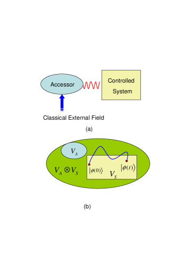
Figure 1: Illustration of indirect quantum control: (a) An external field classically manipulates the quantum accessor and then indirectly controls the quantum system coupling to the accessor with a fixed interaction. (b) When each state in the total Hilbert space $V_{S}\otimes V_{A}$ is reachable under the control via the external classical field acting on the accessor only, each state in the Hilbert space $V_{S}$ must be reachable. This enables a complete controllability for the indirect control of the controlled system

In this paper we utilize the Lie algebra method to systematically study the controllability of the total system formed by the controlled quantum system $\mathcal{S}$ and the quantum accessor $\mathcal{A}$ with Hamiltonian $H_{0}=H_{S}$ $+H_{A}+H_{SA}$. In the theoretic framework of quantum control, it is assumed that the time evolution of the total system can be externally controlled by a family of additional steering fields $\{u_{j}(t)\}$ in a suitable parameter space through the control Hamiltonian

$$H_{c}=\sum_{j}u_{j}(t)W_{j}(a,s).$$ (1)

Here $H_{S}=H_{S}(s)$ ($H_{A}=H_{A}(a)$) is the free Hamiltonian of $\mathcal{S}$ ($\mathcal{A}$) of variable $s$ ($a$) defined on the Hilbert space $V_{S}$ ($V_{A}$) and the coupling Hamiltonian $H_{SA}=H_{SA}(s,a)$ between the system $\mathcal{S}$ and the accessor $\mathcal{A}$ is generally defined on the space $V_{S}\otimes V_{A}$. The control operators $W_{j}(a,s)$ are usually defined also on $V_{S}\otimes V_{A}.$

Obviously it is rather trivial to consider the controllability of the total system of $\mathcal{S}$ and $\mathcal{A}$ when $W_{j}(a,s)$ depends on both $s$ and $a$ since this is essentially the conventional classical control problem of the composite quantum system of $\mathcal{S}$ and $\mathcal{A}$. But it is equally obvious that an important situation will arise if $W_{j}(a,s)$ is constrained to the space of accessor, namely, $\partial_{s}W_{j}(a,s)=0$ or $W_{j}(a,s)=W_{j}(a)$. This case is not at all trivial: it suggests the possibility of controlling the quantum system $\mathcal{S}$ through the control of the variables of the quantum accessor. In fact, this situation is exactly what we will probe in this paper.

We will prove that under some general conditions the control of $\mathcal{A}$ variables can indeed result in a complete quantum control of the whole system and thus lead to an ideal control of its subsystem, the original controlled quantum system $\mathcal{S}$. From mathematical point of view, if the whole system is ergodic in the whole Hilbert space $V_{S}\otimes V_{A}$, then each state in the subspace $V_{S}$ must be reachable by the subsystem $\mathcal{S}$ in the same control process. Here we should point out that a broad dynamical-algebraic framework has been presented, from different motivations and approaches, for analyzing the quantum control properties in terms of the group representation theory z1 ; z2 .

In this paper, the first one of our series papers on indirect quantum control, we shall consider the indirect controllability of arbitrary $N$-energy level quantum system (the qubit) $\mathcal{S}$ through an accessor $\mathcal{A}$ modeled as the spin chain of XY type with nearest neighbor coupling. The controlled system $\mathcal{S}$ and the accessor $\mathcal{A}$ are coupled constantly. We control the system $\mathcal{S}$ by controlling each individual spin of the accessor through a family of external classical fields. To the end of indirect control of quantum system through accessor we also apply a constant classical field to excite the system to be controlled. However, as we will discuss for the case of the 2-dimensional system (see Eq. (34)), such constant excitation can be removed by rotating the controlled system. In the terminology of group theory, this quantum control problem is cased to the Lie group structure hum ; Helgason

$$U(N)_{S}\otimes G_{A}=U(N)_{S}\otimes U(2)_{1}\otimes...\otimes U(2)_{M}.$$ (2)

The remaining part of this paper is organized as follows. In section II, we model the controlled system $\mathcal{S}$ and the accessor $\mathcal{A}$, and formulate the indirect control system. In Section III, we systematically investigate the conditions concerning the complete controllability of the indirect control system, including the coupling between the system and the accessor. In Sections IV and V, we apply the general approach to two and three dimensional cases, respectively. Besides, for the two and three dimensional systems, we will discuss more economical indirect control. Finally, we make a short summary and some remarks in Section VI.

II Indirect quantum control with multi-qubit encoding

First of all, let us point out that throughout this paper the symbol $i$ stands for the complex number $\sqrt{-1}$.

Let $\mathcal{S}$ be the $N$- level quantum system (or qudit) with energy levels $|j\rangle$ ($j=1,2,...,n$), described by the Hamiltonian

$$H_{S}=\sum_{j=1}^{N}E_{j}e_{jj}.$$ (3)

Here $E_{j}$ is the eigen energy and the projection operator $e_{jk}=|j\rangle\langle k|$ stands for the $N\times N$ matrix with the entries $(e_{jk})_{lm}=\delta_{jl}\delta_{km}$. Without losing generality, we suppose that the Hamiltonian $H_{S}$ is traceless, namely tr$H_{S}=0$ or $\sum_{j=1}^{N}E_{j}=0$. Our aim is to answer the question: can we steer the system $\mathcal{S}$ from an initial state to a target state through an intermediate quantum system, the accessor $\mathcal{A}$ and a family of classical fields which control the accessor $\mathcal{A}$ only?

Intuitively, we need a high dimensional accessor $\mathcal{A}$ to control a high dimensional controlled system. We will use a qubit chain to implement this high dimensional accessor $\mathcal{A}$. Suppose that $\mathcal{A}$ consists of $M$ qubits coupled through nearest neighbor interaction with the Hamiltonian $H_{A}=H_{A}^{0}+H_{A}^{\prime}:$

$$H_{A}^{0}=\sum_{j=1}^{M}\hbar\omega_{j}\sigma_{z}^{j},\ \ H_{A}^{\prime}=\sum_{j=1}^{M-1}c_{j}\sigma_{x}^{j}\sigma_{x}^{j+1},$$ (4)

where $c_{j}\neq 0$ is the coupling constant of the nearest neighbor interaction of qubits, $2\hbar\omega_{j}$ is the level spacing of the $j$-th qubit, and $\sigma_{\alpha}^{j}$ ($\alpha=x,y,z$; $j=1,2,\cdots,M$) is the Pauli’s matrix $\sigma_{\alpha}$ of the $j$-th qubit

$$\sigma_{\alpha}^{j}=1\otimes\cdots\otimes 1\otimes\sigma_{\alpha}\otimes 1\otimes\cdots\otimes 1.$$ (5)

The Hamiltonian (4) describes the well known Heisenberg model with nearest neighbor XY-coupling and can be used to simulate a quantum computer by appropriate coding isc . The setup of control system is schematically illustrated in Fig.2.

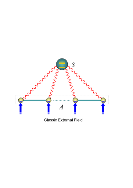
Figure 2: The indirect control system consists of a quantum accessor $\mathcal{A}$ and a $N$-level controlled system $\mathcal{S}$. Here $M$ qubits coupled through nearest neighbor interaction work as the accessor $\mathcal{A}$. We indirectly control the system $\mathcal{S}$ by manipulating the accessor $\mathcal{A}$ with the classic external field.

To control the system $\mathcal{S}$ through $\mathcal{A}$, $\mathcal{S}$ has to be coupled to $\mathcal{A}$. We first excite the system $\mathcal{S}$ by applying a constant classical field on the system $\mathcal{S}$ via the dipole interaction

$$H_{S}^{\prime}=\sum_{j=1}^{N-1}d_{j}x_{j}\otimes 1_{A},$$ (6)

where $d_{j}$’s are time-independent real coupling constants, and $x_{j}$’s are the Hermitian operators defined as $x_{j}=e_{j,j+1}+e_{j+1,j}$. For later use we define $x_{jk}$, $y_{jk}$ ($1\leq j<k\leq N$)and $h_{j}$ as follows:

$$x_{jk}=e_{jk}+e_{kj},$$

$$y_{jk}=i(e_{jk}-e_{kj}),$$

$$h_{j}=e_{j,j}-e_{j+1,j+1}.$$ (7)

Notice that $x_{j}=x_{j,j+1}$ by definition. For this reason, let us define $y_{j}=y_{j,j+1}$. We remark here that with the fixed couplings of $\mathcal{S}$ to an external field, the Hamiltonian of $\mathcal{S}$ can still be diagonalized to take the same form as that of $H_{S}$, but the interaction (4) between $\mathcal{S}$ and $\mathcal{A}$ will then have a complicated form. The skew-Hermitian operators $ix_{jk}$, $iy_{jk}$ and $ih_{j}$ ($1\leq j<k\leq N$)constitute the well-known Chevalley basis of the Lie algebra su($N$) hum . Hereafter we use $1_{S}$ and $1_{A}$ to denote the identity operator on the Hilbert spaces of the system and the accessor respectively.

We note that, different from the conventional control problem, here the interaction $H_{S}^{\prime}$ is time-independent. It seems that the control scenario considered here is not strictly indirect, since there requires a constant control field directly coupling all adjacent transitions of the $N$-level system. However, the excitation by $d_{j}x_{j}\otimes 1_{A}$ can be removed by a transformation of the controlled system, which, in effect, will introduce effective coupling terms to the interaction Hamiltonian $H_{A}^{\prime}$. The explicit proof of this point can be found in Section IV where spin 1/2 is used as an example of the controlled system. We also remark that this constant control field is introduced only for the convenience of the presentations of the lemmas and theorems.

In the following discussion, for convenience for $\alpha_{j}\in\{x,y,z,0\},\,j=1,2,\cdots,M$, we use the abbreviation

$$[\alpha]=(\alpha_{1},\alpha_{2},\cdots,\alpha_{M}),$$

and define

$$\sigma_{[\alpha]}=\prod_{j=1}^{M}\sigma_{\alpha_{j}}^{j},\,\sigma_{0}=1.$$

The coupling between the system $\mathcal{S}$ and the accessor $\mathcal{A}$ is generally given as

$$H_{SA}=\sum_{j=1}^{N-1}\sum_{k=1}^{2}\sum_{[\alpha]}g_{[\alpha]}^{j(k)}s_{j}^{(k)}\otimes\sigma_{[\alpha]},$$ (8)

where in the summation over $[\alpha]$ each $\alpha_{j}$ is restricted to the set $\{x,y\}$, $s_{j}^{(k)}$ ($1\leq j\leq N-1$, $k=1,2$) denotes either $x_{j}$ or $y_{j}$ defined in Eq. (7):

$$s_{j}^{(k)}=\left\{\begin{array}[]{ll}x_{j},&\text{when }k=1,\\ y_{j},&\text{when }k=2,\end{array}\right.$$ (9)

and $g_{[\alpha]}^{j(k)}$ is the coupling constant. The above coupling is general for spin-large spin interaction and reduces to the Heisenberg type coupling when $N=2$.

Then the total system of $\mathcal{S}$ and $\mathcal{A}$ is described by the Hamiltonian $H_{0}$

$$H_{0}=H_{S}\otimes 1_{A}+H_{S}^{\prime}+1_{S}\otimes H_{A}+H_{SA}.$$ (10)

The central point of our protocol is to control the system $\mathcal{S}$ indirectly by controlling the accessor $\mathcal{A}$ using classical fields. Suppose we can completely control every qubit using two independent external fields $f_{j}(t)$ and $f_{j}^{\prime}(t)$, $j=1,2,\cdots,M$, which couple to a qubit in the following way fu1 ; fu2 :

$$H_{x}^{j}=1_{S}\otimes\sigma_{x}^{j},$$ (11)

$$H_{y}^{j}=1_{S}\otimes\sigma_{y}^{j}.$$ (12)

Then the total Hamiltonian for the indirect control is obtained as

$$H=H_{0}+\sum_{j=1}^{M}\left(f_{j}(t)H_{x}^{j}+f_{j}^{\prime}(t)H_{y}^{j}\right).$$ (13)

In this paper we shall examine under what conditions the control system (13) is completely controllable.

III Complete controllability of indirect control

In this section we consider the complete controllability of the system $\mathcal{S}$: whether the system $\mathcal{S}$ can be controlled completely by controlling the accessor $\mathcal{A}$. For this purpose, it is enough to investigate whether the Lie algebra $\mathcal{L}$ generated by $iH_{0}$, $iH_{x}^{j}$ and $iH_{y}^{j}$ is $su$($2^{M}N$), which generates the Lie group of all the unitary operations on $V_{S}\otimes V_{A}$ through the single parameter subgroups. If $\mathcal{L}$ is equal to $su$($2^{M}N$), the system is completely controllable. Otherwise, the system is partly controllable.

For the skew-hermitian operators

$$iH_{0},\ \ \ \ iH_{x}^{j},\ \ \ \ iH_{y}^{j},\ \ j=1,2,...,M$$ (14)

to generate the Lie algebra $su(2^{M}N)$ some conditions should be satisfied. This section is mainly devoted to the investigation of such conditions when $M$ is greater than $2$, the cases with $M=1,2$ being left to the subsequent sections.

For convenience, we introduce the following notions about conditions on the system $\mathcal{S}$:

Condition 1. $c_{j}\neq 0$ for $j=1,2,\cdots,M-1$;

Condition 2. There exist $2(N-1)\equiv N^{\prime}$ elements $[\beta]_{1},[\beta]_{2},\cdots,[\beta]_{N^{\prime}}$ of the set $\{x,y\}^{M}$ such that the matrix

$$G=\left[\begin{array}[]{cccccc}g_{[\beta]_{1}}^{1(1)}&\cdots&g_{[\beta]_{1}}^{(N-1)(1)}&g_{[\beta]_{1}}^{1(2)}&\cdots&g_{[\beta]_{1}}^{(N-1)(2)}\\ g_{[\beta]_{2}}^{1(1)}&\cdots&g_{[\beta]_{2}}^{(N-1)(1)}&g_{[\beta]_{2}}^{1(2)}&\cdots&g_{[\beta]_{2}}^{(N-1)(2)}\\ \cdots&\cdots&\cdots&\cdots&\cdots&\cdots\\ g_{[\beta]_{N^{\prime}}}^{1(1)}&\cdots&g_{[\beta]_{N^{\prime}}}^{(N-1)(1)}&g_{[\beta]_{N^{\prime}}}^{1(2)}&\cdots&g_{[\beta]_{N^{\prime}}}^{(N-1)(2)}\end{array}\right]$$ (15)

is not singular, namely, the determinant of $G$ is nonzero;

Condition 3. The complete controllability conditions on the coupling constants and the eigen-energy $E_{j}$, presented in Ref.[10,11].

Notice that Condition 2 implies the restriction $2^{M}\geq 2(N-1)$.

Lemma 1

Given an arbitrary $[\beta]=(\beta_{1},\beta_{2},\cdots,\beta_{M})\in\{x,y\}^{M}$, we have

$$i^{M}\left[1_{S}\otimes\sigma_{\beta_{M}}^{M},\left[1_{S}\otimes\sigma_{\beta_{M-1}}^{M-1},\left[\cdots,\left[1_{S}\otimes\sigma_{\beta_{1}}^{1},\right.\right.\right.\right.$$

$$\left.\left.i(1_{S}\otimes H_{A}^{\prime})\right]\cdots\right]$$

$$=\left\{\begin{array}[]{ll}4ic_{1}\delta_{\beta_{1}y}\delta_{\beta_{2}y}(1_{S}\otimes\sigma_{z}^{1}\sigma_{z}^{2}),&\text{when }M=2;\\ 0&\text{when }M>2.\end{array}\right.$$ (18)

This lemma can be verified directly. We would rather omit the proof.

Lemma 2

If $i(1_{S}\otimes\sigma_{x}^{j}\sigma_{x}^{j+1})\in\mathcal{L}$ ($j=1,2,\cdots,M-1$), then for an arbitrary $[\alpha]\in\{x,y,z,0\}^{M}$ except $[\alpha]=(0,0,\cdots,0)$ we have $i(1_{S}\otimes\sigma_{[\alpha]})\in\mathcal{L}$.

Proof. We first consider the element $i(1_{S}\otimes\sigma_{[\alpha]})$ with $\alpha_{1}=\alpha_{2}=\cdots=\alpha_{M}=x$. From (11) and (12) we have $1_{S}\otimes\sigma_{y}^{j}\in\mathcal{L}$ and

$$-2^{-1}\left[iH_{x}^{j},iH_{y}^{j}\right]=i(1_{S}\otimes\sigma_{z}^{j})\in\mathcal{L}.$$ (19)

As a result,

$$2^{-1}[i(1_{S}\otimes\sigma_{x}^{2}\sigma_{x}^{3}),\ i(1_{S}\otimes\sigma_{z}^{2})]=i(1_{S}\otimes\sigma_{y}^{2}\sigma_{x}^{3})\in\mathcal{L},$$

$$-2^{-1}[i(1_{S}\otimes\sigma_{x}^{1}\sigma_{x}^{2}),\ i(1_{S}\otimes\sigma_{y}^{2}\sigma_{x}^{3})]=$$

$$\ \ \ \ \ \ i(1_{S}\otimes\sigma_{x}^{1}\sigma_{z}^{2}\sigma_{x}^{3})\in\mathcal{L},$$

$$2^{-1}[i(1_{S}\otimes\sigma_{x}^{1}\sigma_{z}^{2}\sigma_{x}^{3}),i(1_{S}\otimes\sigma_{y}^{2})]=i(1_{S}\otimes\sigma_{x}^{1}\sigma_{x}^{2}\sigma_{x}^{3})\in\mathcal{L}.$$

In the same way we can obtain $i(1_{S}\otimes\sigma_{x}^{1}\sigma_{x}^{2}\sigma_{x}^{3}\sigma_{x}^{4})\in\mathcal{L}$. Now we easily observe that by repeating this procedure we can prove that

$$i(1_{S}\otimes\sigma_{x}^{1}\sigma_{x}^{2}\cdots\sigma_{x}^{M})\in\mathcal{L}.$$ (20)

Next, we consider the elements $i(1_{S}\otimes\sigma_{[\alpha]})$ with $\alpha_{j}\in\{x,y,z\}$. It is easy to see that such elements lie in the Lie algebra generated by $\{i(1_{S}\otimes\sigma_{x}^{1}\sigma_{x}^{2}\cdots\sigma_{x}^{M}),iH_{x}^{j},iH_{y}^{j}|j=1,2,\cdots,M\}$, which is a subset of $\mathcal{L}$. It then follows that $i(1_{S}\otimes\sigma_{[\alpha]})\in\mathcal{L}$ for $\alpha_{j}=x,y,z$.

Finally, we deal with the general element $i(1_{S}\otimes\sigma_{[\alpha]})$ It remains to prove that $i(1_{S}\otimes\sigma_{[\alpha]})\in\mathcal{L}$ for the $\alpha$ with some $\alpha_{j}^{\prime}s$ being zero. To this end, we observe that

$$2^{-1}[i(1_{S}\otimes\sigma_{x}^{1}\sigma_{x}^{2}),\ i(1_{S}\otimes\sigma_{z}^{2})]=i(1_{S}\otimes\sigma_{x}^{1}\sigma_{y}^{2})\in\mathcal{L},$$

so it follows that

$$-2^{-1}\left[i(1_{S}\otimes\sigma_{x}^{1}\sigma_{x}^{2}\cdots\sigma_{x}^{M}),i(1_{S}\otimes\sigma_{x}^{1}\sigma_{y}^{2})\right]$$

$$=i(1_{S}\otimes\sigma_{0}^{1}\sigma_{z}^{2}\sigma_{x}^{3}\cdots\sigma_{x}^{M})\in\mathcal{L}.$$

Now having this element at our disposal, with the help of $iH_{x}^{j}$ and $iH_{y}^{j}$ we can generate in $\mathcal{L}$ all the elements $i(1_{S}\otimes\sigma_{[\alpha]})$ with $\alpha_{1}=0$ and $\alpha_{j}\in\{x,y,z\}$, $j\neq 1$. After a moment’s thought, one can see that using this trick we can actually prove that $i(1_{S}\otimes\sigma_{[\alpha]})\in\mathcal{L}$ for the $\alpha$ with one $\alpha_{j}$, not necessarily $\alpha_{1}$, being zero. Finally, along the same way we can proceed further to show that $i(1_{S}\otimes\sigma_{[\alpha]})\in\mathcal{L}$ for the $\alpha$ with $n$ $\alpha_{j}$’s ($1\leq n<M$) being zero. The lemma is thus proved.

Lemma 3

When $M>2$, if Condition 2 is satisfied, then for $j=1,2,\cdots,N-1$ and $[\alpha]\neq(0,0,\cdots,0)$ the elements $ix_{j}\otimes\sigma_{[\alpha]},iy_{j}\otimes\sigma_{[\alpha]},ih_{j}\otimes 1_{A}$ lie in $\mathcal{L}$.

Proof. We have already known that the elements $i(1_{S}\otimes\sigma_{z}^{j})$($j=1,2,\cdots,M$)are contained in $\mathcal{L}$. So $i(1_{S}\otimes H_{I}^{0})$, which is a linear combination of these elements, is also contained in $\mathcal{L}$. It then follows that $iH_{0}-i(1_{S}\otimes H_{I}^{0})\in\mathcal{L}$, namely,

$$iH_{0}^{\prime}\equiv iH_{S}\otimes 1_{A}+iH_{S}^{\prime}+i(1_{S}\otimes H_{A}^{\prime})+iH_{SA}\in\mathcal{L}.$$ (21)

Now for $\beta_{j}\in\{x,y\}$, let us consider the element

$$i^{M}\left[1_{S}\otimes\sigma_{\beta_{M}}^{M},\left[1_{S}\otimes\sigma_{\beta_{M-1}}^{M-1},\left[\cdots,\left[1_{S}\otimes\sigma_{\beta_{1}}^{1},iH_{0}^{\prime}\right]\cdots\right.\right.\right],$$ (22)

which belongs to $\mathcal{L}$ as $i(1_{S}\otimes\sigma_{\beta_{j}}^{j})$ belongs to $\mathcal{L}$ by definition.

Clearly, the term $i(H_{S}\otimes 1_{A})+iH_{S}^{\prime}$ in $iH_{0}^{\prime}$ has no nonzero contribution to this element. Moreover, since $M>2$ Lemma 1 tells us that the term $i(1_{S}\otimes H_{A}^{\prime})$ has no nonzero contribution either.

By straightforward calculation it then follows that

$$i^{M}\left[1\otimes\sigma_{\beta_{M}}^{M},\left[1\otimes\sigma_{\beta_{M-1}}^{M-1},\left[\cdots,\left[1\otimes\sigma_{\beta_{1}}^{1},iH_{SA}\right]\cdots\right.\right.\right]$$

$$=i(-1)^{M+\Delta}2^{M}\left[\sum_{j=1}^{N-1}\sum_{k=1}^{2}g_{[\bar{\beta}]}^{j(k)}s_{j}^{(k)}\right]\otimes\sigma_{z}^{1}\cdots\ \sigma_{z}^{M}\in\mathcal{L},$$

where $\bar{\beta}$ is defined as

$$\bar{\beta_{j}}=\left\{\begin{array}[]{ll}x,&\text{{if }}\beta_{j}=y,\\ y,&\text{{if }}\beta_{j}=x,\end{array}\right.$$ (23)

and $\Delta$ is the number of $y$ in $\{\beta_{j}|j=1,2,\cdots,M\}$. Consequently, for each $[\beta]\in\{x,y\}^{M}$ we have

$$i\left[\sum_{j=1}^{N-1}\sum_{k=1}^{2}g_{[\bar{\beta}]}^{j(k)}s_{j}^{(k)}\right]\otimes(\sigma_{z}^{1}\cdots\sigma_{z}^{M})\in\mathcal{L}.$$ (24)

There are altogether $2^{M}$ such elements. Now Condition 2 guarantees that from these elements we can choose $2(N-1)$ linearly independent ones. Then from these linearly independent elements in $\mathcal{L}$ we can derive

$$is_{j}^{(k)}\otimes(\sigma_{z}^{1}\cdots\sigma_{z}^{M})\in\mathcal{L},\,j=1,2,\cdots,N-1,\,k=1,2$$ (25)

by the standard method of linear algebra. Using the same method as that in the proof of Lemma 2, we can go further to prove that $is_{j}^{(k)}\otimes\sigma_{[\alpha]}\in\mathcal{L}$, namely, $ix_{j}\otimes\sigma_{[\alpha]},iy_{j}\otimes\sigma_{[\alpha]}\in\mathcal{L}$, for $[\alpha]\neq(0,0,\cdots,0)$. Then the lemma follows directly because we have

$$(-2)^{-1}\left[ix_{j}\otimes\sigma_{[\alpha]},iy_{j}\otimes\sigma_{[\alpha]}\right]=ih_{j}\otimes 1_{A}.$$

Lemma 4

When $M>2$, if Condition 1 and Condition 2 are satisfied, then for $[\alpha]\neq(0,0,\cdots,0)$ we have $i1_{S}\otimes\sigma_{[\alpha]}\in\mathcal{L}$.

Proof. We observe that it follows from Lemma 2 that $iH_{SA}\in\mathcal{L}$ and $iH_{S}\otimes 1_{A}\in\mathcal{L}$. The former is obvious and the latter is due to the fact

$$iH_{S}=i\sum_{j=1}^{N-1}\left(E_{1}+E_{2}+\cdots+E_{j}\right)h_{j},$$ (26)

Recalling that we also have $iH_{A}^{0}\in\mathcal{L}$, we obtain

$$iH_{0}^{\prime\prime}\equiv i\left(H_{0}-H_{S}\otimes 1_{A}-H_{A}-H_{SA}\right)$$ (27)

$$=i1_{S}\otimes\sum_{j=1}^{M-1}c_{j}\sigma_{x}^{j}\sigma_{x}^{j+1}+i\sum_{j=1}^{N-1}d_{j}x_{j}\otimes 1_{A}\in\mathcal{L}.$$

It then follows that

$$\left[\left[iH_{0}^{\prime\prime},iH_{y}^{1}\right],iH_{y}^{1}\right]=-i4c_{1}\left(1_{S}\otimes\sigma_{x}^{1}\sigma_{x}^{2}\right)\in\mathcal{L},$$ (28)

yielding $i\left(1_{S}\otimes\sigma_{x}^{1}\sigma_{x}^{2}\right)\in\mathcal{L}$ thanks to the condition $c_{1}\neq 0$. This leads to the result

$$\left[\left[iH_{0}^{\prime\prime}-ic_{1}1_{S}\otimes\sigma_{x}^{1}\sigma_{x}^{2},\,iH_{y}^{2}\right],\,iH_{y}^{2}\right]$$

$$=-i4c_{2}\left(1_{S}\otimes\sigma_{x}^{2}\sigma_{x}^{3}\right)\in\mathcal{L},$$

namely, $i\left(1\otimes\sigma_{x}^{2}\sigma_{x}^{3}\right)\in\mathcal{L}$ since $c_{2}\neq 0$. Repeating this process we can finally prove

$$i\left(1_{S}\otimes\sigma_{x}^{j}\sigma_{x}^{j+1}\right)\in\mathcal{L},\ \ j=1,2,\cdots,M-1.$$ (29)

Then the lemma follows from Lemma 2.

Theorem 1

When $M>2$, if Condition 1, Condition 2 and Condition 3 are satisfied, then we have $\mathcal{L}=su(2^{M}N)$.

Proof. First we claim that under the conditions of the theorem, for $j=1,2,\cdots,N-1$

$$i\left(x_{j}\otimes 1_{A}\right),i\left(y_{j}\otimes 1_{A}\right)\in\mathcal{L}.$$ (30)

Recall that $iH_{S}\otimes 1_{A}\in\mathcal{L}$ and notice that Eq.(29) implies $iH_{A}^{\prime}\in\mathcal{L}$, and hence

$$iH_{S}^{\prime}=iH_{0}^{\prime\prime}-iH_{A}^{\prime}\in\mathcal{L}.$$

Then according to the result of Ref.[10,11], if Condition 3 is satisfied the elements $i\left(x_{j}\otimes 1_{A}\right)$ and $i\left(y_{j}\otimes 1_{A}\right)$ are contained in the subalgebra of $\mathcal{L}$ generated by $iH_{S}\otimes 1_{A}$ and $iH_{S}^{\prime}$. This proves the claim.

Since the elements of the set $\{ix_{jk},iy_{jk},ih_{j}|1\leq j<k\leq N\}$ can be generated from the set $\{ix_{j},iy_{j}|j=1,2,\cdots,N-1\}$ it follows from Lemma 3, Lemma 4 and (30) that the following elements are in the Lie algebra $\mathcal{L}$

$$ix_{jk}\otimes 1_{A},\ \ y_{jk}\otimes 1_{A},\ \ h_{j}\otimes 1_{A},$$

$$x_{jk}\otimes\sigma_{[\alpha]},\ \ y_{jk}\otimes\sigma_{[\alpha]},\ \ h_{j}\otimes\sigma_{[\alpha]},$$

$$1_{S}\otimes\sigma_{[\alpha]},$$

where $[\alpha]\neq(0,0,\cdots,0)$, and $1\leq j<k\leq N$. It is easily check that these elements are linearly independent and the total number of these elements is

$$(N^{2}-1)+(N^{2}-1)(4^{M}-1)+(4^{M}-1)$$

$$=(2^{M}N)^{2}-1={\dim}\left(su(2^{M}N)\right).$$ (31)

This proves the theorem.

Before leaving this section we would like to note that the coupling between the system and the accessor plays an essential role in the indirect control. In the above given $H_{SA}$ there are $2(N-1)\times 2^{M}$ coupling terms. Actually as far as the controllability is concerned, we have simpler choices of $H_{SA}$. For example, we can reduce the number of coupling terms to $2(N-1)$, just enough to guarantee the satisfaction of Condition 2.

IV Indirect control for two-dimensional system

In this section we will consider an explicit example, the indirect control of a two-energy level system, to illustrate the general approach given in last section. We also present a simpler indirect control scheme for 2-dimensional system.

The 2-dimensional quantum system can be described by the Hamiltonian

$$H_{S}=\hbar\omega_{S}\sigma_{z}\otimes 1_{A},$$ (32)

in terms of Pauli’s matrices. In this case, it is possible to use just one qubit as the accessor. The Hamiltonian of the entire control system can be written as

$$H =\hbar\omega_{S}\sigma_{z}\otimes 1_{A}+g\sigma_{x}\otimes 1+1_{S}\otimes\hbar\omega_{I}\sigma_{z}$$

$$+g_{xx}\sigma_{x}\otimes\sigma_{x}+g_{xy}\sigma_{x}\otimes\sigma_{y}$$

$$+g_{yx}\sigma_{y}\otimes\sigma_{x}+g_{yy}\sigma_{y}\otimes\sigma_{y}$$

$$+f_{1}(t)\left(1_{S}\otimes\sigma_{x}\right)+f_{2}(t)\left(1_{S}\otimes\sigma_{y}\right).$$ (33)

Here we remark that the excitation term $\sigma_{x}\otimes 1$ can be removed by rotating the controlled system around y-direction so that $\hbar\omega_{S}\sigma_{z}\otimes 1_{A}+g\sigma_{x}\otimes 1$ becomes $\hbar\omega_{S}^{\prime}\sigma_{z}\otimes 1_{A}$ . As the price paid, the rotated Hamiltonian contains the terms $g_{zx}^{\prime}\sigma_{z}\otimes\sigma_{x}$ and $g_{zy}^{\prime}\sigma_{z}\otimes\sigma_{y}$ (see Fig.3):

$$H =\hbar\omega_{S}^{\prime}\sigma_{z}\otimes 1_{A}+1_{S}\otimes\hbar\omega_{I}\sigma_{z}$$

$$+g_{xx}^{\prime}\sigma_{x}\otimes\sigma_{x}+g_{xy}^{\prime}\sigma_{x}\otimes\sigma_{y}$$

$$+g_{yx}\sigma_{y}\otimes\sigma_{x}+g_{yy}\sigma_{y}\otimes\sigma_{y}$$

$$+g_{zx}^{\prime}\sigma_{z}\otimes\sigma_{x}+g_{zy}^{\prime}\sigma_{z}\otimes\sigma_{y}$$

$$+f_{1}(t)\left(1_{S}\otimes\sigma_{x}\right)+f_{2}(t)\left(1_{S}\otimes\sigma_{y}\right).$$ (34)

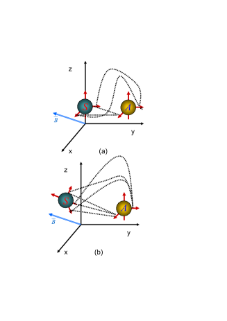
Figure 3: (a) There are 4 terms (denoted by 4 dotted lines ) in the interaction between the controlled qubit (green) and the quantum accessor (yellow) when a constant field $\vec{B}$ is applied in the x-direction ; (b) After the controlled qubit is rotated to be along the direction of the total external field there will be 6 terms in the interaction, which are denoted by 6 dotted lines.

The following theorem is the main result of this section.

Theorem 2

Suppose that $g_{xy}g_{yx}\neq g_{xx}g_{yy}$. Then the symplectic Lie algebra sp(4) is included in $\mathcal{L}$. Moreover, if $g\neq 0$ is also satisfied, then $\mathcal{L}=su(4)$.

Proof. We observe that in the present case, Lemma 1 reduces to the trivially true identity since the coupling term in $H_{A}$ does not appear. On the other hand the assumption $g_{xy}g_{yx}\neq g_{xx}g_{yy}$ simply means that Condition 2 is satisfied. Therefore Lemma 2 is valid. Noticing that,by definition, $x_{1}=\sigma_{x}$, $y_{1}=\sigma_{y}$ and $h_{1}=\sigma_{z}$ with respect to a proper basis when $N=2$, we conclude, from Lemma 2 and the fact that $\mathcal{L}$ contains the elements $i(1_{S}\otimes\sigma_{x})$ $i(1_{S}\otimes\sigma_{x})$ by definition, that $\mathcal{L}$ contains the following elements:

$$i(1_{S}\otimes\sigma_{\alpha}),\ \ \ \alpha=x,y,z;$$

$$i\sigma_{\alpha}\otimes\sigma_{\beta},\ \ \ \alpha=x,y,\beta=x,y,z;$$

$$i(\sigma_{z}\otimes 1_{A})$$ (35)

and thus contains the element $g(i\sigma_{x}\otimes 1_{A})$, which is obtained by subtracting from $iH_{0}$ all the other terms, which lie in $\mathcal{L}$.

Now we claim that we can choose a basis of sp(4) from those elements in (35). In fact, we have

-ii),i​(1⊗σz)=( -i-i),formulae-sequencetensor-product𝑖subscript𝜎𝑧1fragments fragments missing-subexpressionmissing-subexpression-imissing-subexpressionmissing-subexpressionmissing-subexpressionmissing-subexpressioni𝑖tensor-product1subscript𝜎𝑧fragments fragments missing-subexpressionmissing-subexpression-imissing-subexpressionmissing-subexpressionmissing-subexpressionmissing-subexpression-ii\sigma_{z}\otimes 1=\left(\begin{tabular}[]{cc|cc}i&&&\\ &-i&&\\ \hline\cr&&-i&\\ &&&i\end{tabular}\right),i(1\otimes\sigma_{z})=\left(\begin{tabular}[]{cc|cc}i&&&\\ &i&&\\ \hline\cr&&-i&\\ &&&-i\end{tabular}\right),

i-iiii-iii (36)

-i-i),i​σy⊗σz=( -11),formulae-sequencetensor-product𝑖subscript𝜎𝑥subscript𝜎𝑧fragments fragments missing-subexpressionmissing-subexpressionmissing-subexpression-imissing-subexpressionmissing-subexpression-imissing-subexpressiontensor-product𝑖subscript𝜎𝑦subscript𝜎𝑧fragments fragments missing-subexpressionmissing-subexpressionmissing-subexpression-1missing-subexpressionmissing-subexpression1missing-subexpressioni\sigma_{x}\otimes\sigma_{z}=\left(\begin{tabular}[]{cc|cc}&i&&\\ i&&&\\ \hline\cr&&&-i\\ &&-i&\end{tabular}\right),i\sigma_{y}\otimes\sigma_{z}=\left(\begin{tabular}[]{cc|cc}&1&&\\ -1&&&\\ \hline\cr&&&-1\\ &&1&\end{tabular}\right),

ii1-1ii1-1 (37)

ii),i​σx⊗σy=( -1-1),formulae-sequencetensor-product𝑖subscript𝜎𝑥subscript𝜎𝑥fragments fragments imissing-subexpressionmissing-subexpressionmissing-subexpressionmissing-subexpressionimissing-subexpressionmissing-subexpressiontensor-product𝑖subscript𝜎𝑥subscript𝜎𝑦fragments fragments -1missing-subexpressionmissing-subexpressionmissing-subexpressionmissing-subexpression-1missing-subexpressionmissing-subexpressioni\sigma_{x}\otimes\sigma_{x}=\left(\begin{tabular}[]{cc|cc}&&i&\\ &&&i\\ \hline\cr i&&&\\ &i&&\end{tabular}\right),i\sigma_{x}\otimes\sigma_{y}=\left(\begin{tabular}[]{cc|cc}&&1&\\ &&&1\\ \hline\cr-1&&&\\ &-1&&\end{tabular}\right),

ii11ii11 (38)

-11),i​σy⊗σy=( -ii),formulae-sequencetensor-product𝑖subscript𝜎𝑦subscript𝜎𝑥fragments fragments -1missing-subexpressionmissing-subexpressionmissing-subexpressionmissing-subexpression1missing-subexpressionmissing-subexpressiontensor-product𝑖subscript𝜎𝑦subscript𝜎𝑦fragments fragments fragments-imissing-subexpressionmissing-subexpressionmissing-subexpressionmissing-subexpressionimissing-subexpressionmissing-subexpressioni\sigma_{y}\otimes\sigma_{x}=\left(\begin{tabular}[]{cc|cc}&&1&\\ &&&-1\\ \hline\cr-1&&&\\ &1&&\end{tabular}\right),i\sigma_{y}\otimes\sigma_{y}=\left(\begin{tabular}[]{cc|cc}&&-i&\\ &&&i\\ \hline\cr-i&&&\\ &i&&\end{tabular}\right),

1-1-ii1-1-ii (39)

ii),i​(1⊗σy)=( -1-1),formulae-sequence𝑖tensor-product1subscript𝜎𝑥fragments fragments missing-subexpressionimissing-subexpressionmissing-subexpressionimissing-subexpressionmissing-subexpressionmissing-subexpression𝑖tensor-product1subscript𝜎𝑦fragments fragments missing-subexpression-1missing-subexpressionmissing-subexpression-1missing-subexpressionmissing-subexpressionmissing-subexpressioni(1\otimes\sigma_{x})=\left(\begin{tabular}[]{cc|cc}&&&i\\ &&i&\\ \hline\cr&i&&\\ i&&&\end{tabular}\right),i(1\otimes\sigma_{y})=\left(\begin{tabular}[]{cc|cc}&&&1\\ &&1&\\ \hline\cr&-1&&\\ -1&&&\end{tabular}\right),

ii11ii11 (40)

with respect to the ordered basis $\{|0\rangle\otimes|0\rangle,|1\rangle\otimes|0\rangle,|1\rangle\otimes|1\rangle,|0\rangle\otimes|1\rangle\}$. It is readily check that these matrices are linearly independent and satisfy the equation

$$S^{t}x+xS=0,$$ (41)

the defining relation of $sp(4)$, where

$$S=\left(\begin{array}[]{cc}&I\\ -I&\end{array}\right)$$ (42)

and $I$ is the $2\times 2$ identity matrix. This proves the claim, and hence the first part of the theorem, as the dimension of $sp(4)$ is $10$.

If $g\neq 0$, from $g(i\sigma_{x}\otimes 1_{A})\in\mathcal{L}$ we can derive $i\sigma_{x}\otimes 1_{A}\in\mathcal{L}$. It is easily check that this element, together with the elements in (35), can generate $15$ linearly independent elements by Lie bracket operations. As the dimension of $su(4)$ is exactly $15$ we conclude that $\mathcal{L}=su(4)$. The proof of Theorem 2 is thus completed.

We remark that it is easy to satisfy the condition $g_{xy}g_{yx}\neq g_{xx}g_{yy}$. For example, we can take

$$g_{xx}=g_{yy}=0,g_{xy}=g_{yx}\neq 0,$$ (43)

or

$$g_{xy}=g_{yx}=0,g_{xx}=g_{yy}\neq 0.$$ (44)

In both cases, there are only two terms in the coupling between the system $\mathcal{S}$ and the accessor $\mathcal{A}$.

Finally, we point out that, by making full use of the property that the square of Pauli’s matrices is unity, which is peculiar to the $N=2$ case, we can manage to control the system completely by means of simpler couplings between the system and the accessor. Let us consider, as an example, the control system

$$H_{0} =\hbar\omega_{S}\sigma_{z}\otimes 1_{A}+g\sigma_{x}\otimes 1$$

$$+1_{S}\otimes\hbar\omega_{I}\sigma_{z}+g_{xx}\sigma_{x}\otimes\sigma_{x},$$ (45)

$$H_{c} =f_{1}(t)\left(1_{S}\otimes\sigma_{x}\right)+f_{2}(t)\left(1_{S}\otimes\sigma_{y}\right)$$

where $g\neq 0$ and $g_{xx}\neq 0$. Such a control system is essentially different from the system just discussed above as in this case Condition 2 is never satisfied. One can easily check that

$$(2g_{xx})^{-1}\left(-[iH_{0},i(1\otimes\sigma_{y})]+2i\hbar\omega_{I}\otimes\sigma_{x}\right)$$

$$=i\sigma_{x}\otimes\sigma_{z}\in\mathcal{L},$$ (46)

from which we further have

$$-(2\hbar\omega_{S})^{-1}\left[iH_{0}-\hbar\omega_{I}1\otimes\sigma_{z}-ig_{xx}\sigma_{x}\sigma_{x},\ i\sigma_{x}\otimes\sigma_{z}\right]$$

$$=(2\hbar\omega_{S})^{-1}\left[\hbar\omega_{S}\sigma_{z}\otimes 1_{A}+g\sigma_{x}\otimes 1,\ \sigma_{x}\otimes\sigma_{z}\right]$$

$$=i\sigma_{y}\otimes\sigma_{z}\in\mathcal{L}.$$ (47)

Now it should not be difficult to proceed further to prove that the two conclusions of Theorem 2 are still valid though the premise is no longer true. We leave the details to interested readers.

V Indirect control for 3-dimensional quantum system

In this section we discuss the indirect control of 3-dimensional quantum system based on the approach presented in Section III.

Since Theorem 1 is, generally speaking, not valid when $M\leq 2$, we first consider the possibility of using 3 qubits to control the system, namely, we assume that $M=3$.

Let $[\beta]_{1}=(x,x,x)$, $[\beta]_{2}=(x,x,y)$, $[\beta]_{3}=(x,y,x)$ and $[\beta]_{4}=(y,x,x)$. To satisfy Condition 2, we can simply choose $g_{[\beta]}^{j(k)}=0$ except that

$$g_{[\beta]_{1}}^{1(1)}=g_{[\beta]_{2}}^{2(1)}=g_{[\beta]_{3}}^{1(2)}=g_{[\beta]_{4}}^{2(2)}=1,$$ (48)

namely,

$$H_{SA} =x_{1}\otimes\sigma_{y}^{1}\sigma_{y}^{2}\sigma_{y}^{3}+x_{2}\otimes\sigma_{y}^{1}\sigma_{y}^{2}\sigma_{x}^{3}$$

$$+y_{1}\otimes\sigma_{y}^{1}\sigma_{x}^{2}\sigma_{y}^{3}+y_{2}\otimes\sigma_{x}^{1}\sigma_{y}^{2}\sigma_{y}^{3}.$$ (49)

In fact, in such a case, we have

$$\det\left[\begin{array}[]{cccc}g_{[\beta]_{1}}^{1(1)}&g_{[\beta]_{1}}^{2(1)}&g_{[\beta]_{1}}^{1(2)}&g_{[\beta]_{1}}^{2(2)}\\ g_{[\beta]_{2}}^{1(1)}&g_{[\beta]_{2}}^{2(1)}&g_{[\beta]_{2}}^{1(2)}&g_{[\beta]_{2}}^{2(2)}\\ g_{[\beta]_{3}}^{1(1)}&g_{[\beta]_{3}}^{2(1)}&g_{[\beta]_{3}}^{1(2)}&g_{[\beta]_{3}}^{2(2)}\\ g_{[\beta]_{4}}^{1(1)}&g_{[\beta]_{4}}^{2(1)}&g_{[\beta]_{4}}^{1(2)}&g_{[\beta]_{4}}^{2(2)}\end{array}\right]=1$$ (50)

Now assume Condition 1, then Condition 3 is enough to guarantee the complete controllability. In our present case, Condition 3 has a simple formfu1 ; fu2 :

$$\Delta_{21}^{2}\neq\Delta_{32}^{2}\text{ and }d_{1}\neq 0,d_{2}\neq 0$$ (51)

or

$$\Delta_{21}^{2}=\Delta_{32}^{2}\text{ and }d_{1}\neq\pm d_{2}\neq 0,$$ (52)

where $\Delta_{jk}\equiv E_{j}-E_{k}$ ($3\geq j>k\geq 1$) is the energy gap.

Now we consider the possibility of using only two qubits to control the 3-dimensional system. As in this case $M=2$, the general approach developed in Section III cannot be fully applied. However, we have the following conclusion: if we can control not only each qubit, but also their coupling independently, we can indirectly control the 3-dimensional system using two qubits. In fact, if this is the case, we can take the Hamiltonian as

$$H =H_{0}+H_{c}^{1}+H_{c}^{2}+H_{c}^{12}$$

$$H_{0} =\sum_{j=1}^{3}\hbar\omega_{S}e_{jj}\otimes 1_{A}+\left(d_{1}x_{1}+d_{2}x_{2}\right)\otimes 1_{A}$$

$$+1_{S}\otimes\sum_{j=1}^{2}(\hbar\omega_{I}\sigma_{z}^{j})$$ (53)

$$+\sum_{j=1}^{2}\sum_{\alpha_{1},\alpha_{2}=x,y}g_{\alpha_{1}\alpha_{2}}^{j(k)}s_{j}^{(k)}\otimes(\sigma_{\alpha_{1}}^{1}\sigma_{\alpha_{2}}^{2})$$

$$H_{c}^{j} =f_{j}(t)\left(1_{S}\otimes\sigma_{x}^{j}\right)+f_{j}^{\prime}(t)\left(1_{S}\otimes\sigma_{y}^{j}\right)$$

$$H_{c}^{12} =f(t)1_{S}\otimes\sigma_{x}^{1}\sigma_{x}^{2}.$$ (54)

Let $\mathcal{L}$ be the Lie algebra generated by the elements

$$iH_{0},\ \ \ i\left(1_{S}\otimes\sigma_{x}^{j}\right),\ \ \ i\left(1_{S}\otimes\sigma_{y}^{j}\right),\ \ \ i\left(1\otimes\sigma_{x}^{1}\sigma_{x}^{2}\right),$$ (55)

where $j=1,2$. Then mathematically the complete controllability condition is $\mathcal{L}=su(4)$. Using a method similar to that in Section III we can prove $\mathcal{L}=su(4)$ if the condition(51) or (52), and the condition

$$\det\left[\begin{array}[]{cccc}g_{xx}^{1(1)}&g_{xx}^{2(1)}&g_{xx}^{1(2)}&g_{xx}^{2(2)}\\ g_{xy}^{1(1)}&g_{xy}^{2(1)}&g_{xy}^{1(2)}&g_{xy}^{2(2)}\\ g_{yx}^{1(1)}&g_{yx}^{2(1)}&g_{yx}^{1(2)}&g_{yx}^{2(2)}\\ g_{yy}^{1(1)}&g_{yy}^{2(1)}&g_{yy}^{1(2)}&g_{yy}^{2(2)}\end{array}\right]\neq 0$$ (56)

are satisfied. We would rather omit the details to avoid redundancy.

Finally, we conclude this section by pointing out that (56) can be satisfied by simply choosing

$$H_{SA}^{\prime} =x_{1}\otimes\sigma_{x}^{1}\sigma_{x}^{2}+y_{1}\otimes\sigma_{x}^{1}\sigma_{y}^{2}$$

$$+x_{2}\otimes\sigma_{y}^{1}\sigma_{x}^{2}+y_{2}\otimes\sigma_{y}^{1}\sigma_{y}^{2}.$$ (57)

VI Conclusion and remarks

In this paper we investigated the controllability of an arbitrary finite dimensional quantum system via a quantum accessor modeled as a spin chain with nearest neighbor coupling of XY-type. The general approach is applied to the indirect control of two and three dimensional quantum systems. We also present indirect control schemes simpler than the general scheme for two and three dimensional systems. Our approach shows that one can completely control an finite-dimensional quantum system through a quantum accessor if the system and the accessor are coupled properly.

We point out that we have supposed that each spin of the quantum accessor can be individually controlled. In forthcoming paper we would like to explore the indirect control of the quantum systems by controlling the accessor globally. Global control of spin chains itself has been studied recently in the context of quantum computation global . It is definitely of interest to realize the indirect control by global control of quantum accessor. In Sec. IV we found that we can achieve the indirect control without applying the constant excitation field to the system by rotating the system around y-direction (see Eq. (34)). This example suggests us removing the excitation field from the controlled system to achieve the pure indirect control. We will address this issue in our forthcoming paper. Obviously it is also significant study a control system where the fixed interaction between the controlled system and the accessor is so weak that it can be neglected approximately when the strong field, which controls the accessor, is switched on.

Before concluding this paper we would like to remark that in the conventional investigation on the controllability of quantum systems, the controls are usually classical or semiclassical since the controlling field is described as a time-dependent functions and directly affects the time evolution of the closed or open quantum systems to be controlled albe ; viol1 ; viol2 ; alta ; Rama . So it might be more appropriate to name those types of control (semi)classical control of quantum systems.

References

• (1) Information Complexity and Control in Quantum Physics, edited by A. Blaquiere, S. Dinerand and G. Lochak (Springer, New York, 1987)
• (2) A. G. Butkovskiy and Yu. I. Samoilenko, Control of Quantum-mechanical Processes and Systems (Kluwer Academic, Dordrecht, 1990)
• (3) V. Jurdjevic, Geometric Control Theory, Cambridge University Press, 1997
• (4) S. Lloyd, Phys. Rev. A 62, 022108 (2000)
• (5) G. M. Huang, T. J. Tarn and J. W. Clark, J. Math. Phys. 24, 2608 (1983)
• (6) M. A. Nielsen and I. L. Chuang, Quantum Computation and Quantum Information (Cambridge University Press, 2000)
• (7) V. Ramakrishna and H. Rabitz, Phys. Rev. A 54, 1715-1716 (1996)
• (8) Fei Xue, S.X. Yu, C.P. Sun Phys. Rev. A 73, 013403 (2006)
• (9) R.-B. Wu, T.-J. Tarn, and C.-W. Li, Phys. Rev. A 73, 012719 (2006)
• (10) H. Fu, S. G. Schirmer and A. I. Solomon, J. Phys. A. 34 (2001) 1679.
• (11) S. G. Schirmer, H. Fu and A. I. Solomon, Phys. Rev. A. 63 (2001) 063410.
• (12) R. Romano and D. D’Alessandro, Phys. Rev. A 73, 022323 (2006)
• (13) R. Romano and D. D’Alessandro, Phys. Rev. Lett. 97, 080402 (2006)
• (14) R. Vilela Mendes and V. I. Mano, Phys. Rev. A 67, 053404 (2003)
• (15) A. Mandilara and J. W. Clark, Phys. Rev. A 71, 013406 (2005)
• (16) P. Zanardi and S. Lloyd, Phys. Rev. A 69, 022313 (2004)
• (17) P. Giorda, P. Zanardi, and S. Lloyd, Phys. Rev. A 68, 062320 (2003).
• (18) J. E, Humphreys, Introduction to Lie Algebras and Representation Theory, Spring-Verlag New York, 1972
• (19) S. Helgason, Differential Geometry, Lie Groups and Symmetric Spaces (Academic Press, 1978)
• (20) F. Albertini and D. Dlessandro, IEEE Transactions on Automatic Control 48, 1399 (2003)
• (21) L. Viola, S. Lloyd and E. Knill, Phys. Rev. Lett. 83, 4888 (1999)
• (22) L. Viola and S. Lloyd, Phys. Rev. A 65, 010101 (2002)
• (23) C. Altafini, J. Math. Phys. 44, 2357 (2003)
• (24) V. Ramakrishna, M. Salapaka, M. Dahleh, H. Rabitz and A. Peirce, Phys. Rev. A 51, 960 (1995)
• (25) D. A. Lidar, D. Bacon and K. B. Whaley, Phys. Rev. Lett. 82,4556 (1999); D. P. DiVincenzo, D. Bacon, J. Kempe, G. Burkard and K. B. Whaley, Nature 408, 339 (2000).
• (26) Z.-W. Zhou,Y.-J. Han and G.-C. Guo, quant-ph/0610168 and references therein.