Local Operations in qubit arrays via global but periodic Manipulation

Abstract

We provide a scheme for quantum computation in lattice systems via global but periodic manipulation, in which only effective periodic magnetic fields and global nearest neighbor interaction are required. All operations in our scheme are attainable in optical lattice or solid state systems. We also investigate universal quantum operations and quantum simulation in 2 dimensional lattice. We find global manipulations are superior in simulating some nontrivial many body Hamiltonians.

I Introduction

Since a quantum computer (QC) will exhibit advantages over its classical counterpart only when a large number of qubits can be manipulated coherently, many architectures of QCs based on scalable physical systems have been investigatedSQC1 ; SQC2 ; SQC3 ; SQC4 ; SQC5 . Among these candidates, ultra-cold neutral atoms trapped in the periodic potentials of an optical lattice are attracting much attentionSQC5 ; SQC6 ; SQC7 ; SQC8 ; Cold-atom1 ; Cold-atom2 ; Cold-atom3 ; Cold-atom4 . Since neutral atoms couple weakly to the environment, decoherence is suppressed greatly. Besides, some typical many-body models can be constructed in optical lattice systems. This makes it possible to use quantum optical methods to study fundamental condensed-matter physics problemsCold-atom5 ; Cold-atom6 ; Cold-atom7 ; Cold-atom8 .

In the schemes for QCs based on optical lattice system, the couplings between nearest neighbor atoms in the lattice can be simultaneously switched on and off by adjusting the intensity, frequency, and polarization of the trapping light. However, it is difficult to focus a laser beam on a single atom due to the short lattice period. This makes it challenging to realize controlled collisions and perform single and two qubit logical operations. A possible approach to overcome the difficulty of addressing the atoms individually is based on marker qubitsSQC6 ; SQC7 ; SQC8 , i.e., by using two types of atoms with different internal states in the optical lattice. One type of atoms act as marker qubits to address logical qubits. Another method is one way quantum computationoneway . In this proposal, the couplings between adjacent atoms can be utilized to prepare the atoms in a high dimensional cluster state. After the initialization, one can enlarge the lattice period to single qubit addressable range. Universal quantum computation can then be implemented simply via a series of single qubit measurements. Of course, one way quantum computation requires a great qubit overhead.

Recently, a series of schemes for quantum computation based on global operations only were proposed. In these schemes, local addressability become unnecessaryLloyd ; Benjamin ; Wu ; Raussendorf ; Cirac ; Nagy . Remarkably, Raussendorf devised a novel scheme for universal quantum computation via translation-invariant operations on a chain of qubitsRaussendorf , in which only the nearest neighbor Ising-type interaction and translation-invariant single qubit unitary operations are required. Inspired by these proposals, in this letter we present a scheme for quantum computation based on global operations in qubit arrays only. Here, we develop a general method to realize single qubit unitary operations via global but periodic manipulation. Compared with the quantum cellular automata schemeLloyd ; Benjamin , encoding overhead is eliminated in our proposal. In addition, single qubit operation is easier than in Raussendorf’s schemeRaussendorf .

The paper is organized as follows. In Sec.II, we show that universal quantum computation in one dimensional arrays can be realized via global but periodic manipulation. We also display that the preparation for initial states and the measurement for final states can be implemented by using this global manipulation. Furthermore, in Sec.III, we discuss quantum computation and quantum simulation in high dimensional arrays. We find the implementation of the periodic operations in the finite lattice will benefit from global manipulation. Section IV contains some conclusions.

II Universal quantum computation in one dimensional arrays

Let us first consider a two-component bosonic atomic mixture trapped in one dimension by two spin-dependent lattice potentials. Each atom is assumed to have two relevant internal states, which are denoted with the effective spin index $\sigma=\uparrow$, $\downarrow$, respectively. In the Mott insulator regime, the system can be described by a two-component Bose-Hubbard HamiltonianSQC5 :

$$H = -\sum_{i,\sigma}(t_{\sigma}a_{i\sigma}^{+}a_{i+1\sigma}+H.c.)+\frac{1}{2}\sum_{i,\sigma}U_{\sigma}n_{i\sigma}(n_{i\sigma}-1)$$ (1)

$$+U_{\uparrow\downarrow}\sum_{i}n_{i\uparrow}n_{i\downarrow}.$$

Here, $a_{i\sigma}^{+}$ and $a_{i\sigma}$ are creation and annihilation operators for bosonic atoms of spin $\sigma$ localized on-site $i$, and $n_{i\sigma}=a_{i\sigma}^{+}a_{i\sigma}$. Under the condition that $t_{\sigma}\ll U_{\sigma},U_{\uparrow\downarrow}$ and $\left\langle n_{i\uparrow}\right\rangle+\left\langle n_{i\downarrow}\right\rangle=1$, Eq. (1) is equivalent to the following $XXZ$ type interaction HamiltonianSQC5 ; Kuklov :

$$H_{S}=\sum_{i}\left[J_{1}\sigma_{i}^{z}\sigma_{i+1}^{z}-J_{2}(\sigma_{i}^{x}\sigma_{i+1}^{x}+\sigma_{i}^{y}\sigma_{i+1}^{y})\right].$$ (2)

Here, $\sigma_{i}^{z}=n_{i\uparrow}-n_{i\downarrow}$, $\sigma_{i}^{x}=a_{i\uparrow}^{+}a_{i\downarrow}+a_{i\downarrow}^{+}a_{i\uparrow}$, and $\sigma_{i}^{y}=-i(a_{i\uparrow}^{+}a_{i\downarrow}-a_{i\downarrow}^{+}a_{i\uparrow})$ satisfy $\left[\sigma_{i}^{\alpha},\sigma_{i}^{\beta}\right]=2i\epsilon_{\alpha\beta\gamma}\sigma_{i}^{\gamma}$. $J_{1}=(t_{\uparrow}^{2}+t_{\downarrow}^{2})/2U_{\uparrow\downarrow}-t_{\uparrow}^{2}/U_{\uparrow}-t_{\downarrow}^{2}/U_{\downarrow}$, $J_{2}=t_{\uparrow}t_{\downarrow}/U_{\uparrow\downarrow}$. Remarkably, the parameters $J_{1}$ and $J_{2}$ can be easily controlled by adjusting the intensity of the trapping laser beam or an external fieldSQC5 . Therefore, the following well-known spin $1/2$ interaction models can be realized: Ising model $\left(J_{1}\neq 0,J_{2}=0\right)$, $XY$ model $\left(J_{1}=0,J_{2}\neq 0\right)$, and Heisenberg antiferromagnetic (ferromagnetic) model $\left(J_{1}=\pm J_{2}\right)$.

Besides Hamiltonian $H_{S}$, in order to implement universal quantum computation, we introduce the following effective periodic magnetic field:

$$H_{B}^{\alpha}(a,\varphi)=\sum_{i}A\left[1-\cos\left(\frac{2\pi i}{a}+\varphi\right)\right]\sigma_{i}^{\alpha},(\alpha=x,y,z)$$ (3)

Here, we set the distance between the nearest neighbor sites as unity. $a$ is the period of the magnetic field, when $a\rightarrow\infty$, $H_{B}^{\alpha}(a,\varphi)$ reduces to a homogeneous magnetic field. To realize this periodic magnetic field, we set the eigenstates $\left|\uparrow\right\rangle$ and $\left|\downarrow\right\rangle$ to have the same energy. By the left and the right circularly polarized light, they are separately coupled to the common exited level $\left|e\right\rangle$ with a blue detuning $\Delta$. In such a 3-level system, we can obtain the effective Hamiltonians $\sigma_{x}$, $\sigma_{y}$, and $\sigma_{z}$ in the 2 dimensional Hilbert space spanned by $\left|\uparrow\right\rangle$ and $\left|\downarrow\right\rangle$ only by adjusting the polarization of coupling lightSQC5 . Thus, for the cold atoms trapped in one dimensional lattice, we may construct such a periodic potential field $H_{B}^{\alpha}(a,\varphi)$ along the lattice direction by applying a monochromatic standing wave laser beam. In addition, in our scheme, we require the ability to adjust the period of the effective magnetic field $H_{B}^{\alpha}(a,\varphi)$. To this end, we split a beam of monochromatic light into two beams and make them interfere. Thus, we can obtain a one dimensional standing wave along the interior bisector of the angle between two beams of lights, whose period depends on the angle between the two beams of lights.

II.1 Single qubit operations

Here, we present a general method to control any single qubit on one-dimensional finite lattice by using global Hamiltonian $H_{B}^{\alpha}(a,\varphi)$. Our idea for local manipulation derives from Fourier transformation i.e., any spatial function can be decomposed into a superposition of periodic eigen-functions. Let us consider a one-dimensional chain of $N$ qubits. The unitary evolution controlled by the effective periodic magnetic filed $H_{B}^{\alpha}(a,\varphi)$ is: $U_{1}(\theta,a,k,\alpha)=\exp\left\{-i\frac{\theta}{A}H_{B}^{\alpha}(a,\frac{-2\pi k}{a})\right\}$. Our aim is to implement a delta function type of operation on the finite spin chain by assembling these wave-like unitary operations $U_{1}(\theta,a,k,\alpha)$. Without loss of generality, we consider performing a unitary operation $\exp(-i\theta\sigma_{k}^{x})$ on the $k$th site. The operation on a single site can be realized in an iterative way. In the iterative procedure, a key step is to construct parity unitary operation: $F_{k}^{(1)}=U_{1}(\pi/4,2,k,z)F_{k}^{(0)}U_{1}^{*}(\pi/4,2,k,z)F_{k}^{(0)}=\prod_{\lceil\frac{k-1}{2}\rceil\leq j\leq\lceil\frac{N-k}{2}\rceil}\exp(-i2\theta\sigma_{k+2j}^{x}).$ Here, $\lceil\eta\rceil$ refers to the integer part of the number $\eta$ and $F_{k}^{(0)}=\exp\left\{-i\frac{\theta}{2A}H_{B}^{x}(\infty,\pi)\right\}$. The parity unitary operation $F_{k}^{(1)}$ only remains homogeneous on even sites array from the $k$th site. It effectively just implements a homogeneous operation on a spin chain of $N/2$ qubits. We find that similar parity-eliminated operations can be established iteratively: $F_{k}^{(l)}=U_{1}(\pi/4,2^{l},k,z)F_{k}^{(l-1)}U_{1}^{*}(\pi/4,2^{l},k,z)F_{k}^{(l-1)},$ $1\leq l\leq m,m=\lceil\log_{2}\left(N-k\right)\rceil+1.$ Finally, operation on the $k$th qubit can be realized: $F_{k}^{(m)}=$ $\exp(-i2^{m}\theta\sigma_{k}^{x})$ (see Fig. 1(a)). In this iterative procedure, implementing single qubit rotation takes $3\times 2^{m}-2$ elementary steps (applications of $U_{1}(\theta,a,k,\alpha)$), which roughly ranges from $1.5N$ to $6N$.

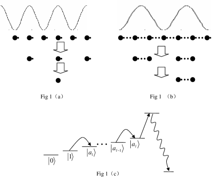
Figure 1: Schematic for addressing and readout measurements via global operations. (a) The process of single qubit operation. In an iterative step, approximately half sites are selected out. (b) A high efficiency procedure for operation between two nearest neighbor sites. In an iterative step, approximately two thirds couplings in the remaining spin chain are eliminated. (c) Mapping quantum states $\left|1\right\rangle$ localized in far apart sites into auxiliary energy level $\left|a_{l}\right\rangle$ by using modified periodic magnetic fields. The read out for state $\left|a_{l}\right\rangle$ can be implemented by the method of detecting the fluorescence.

II.2 Two-qubit operations

Since single qubit operations can be realized, implementing two-qubit operation between two nearest neighbor qubits via many body interaction becomes feasible. We consider the case of Ising model: $H_{I\sin g}=\sum_{i=1}^{N-1}J_{1}\sigma_{i}^{z}\sigma_{i+1}^{z}$. When the couplings between nearest neighbor qubits switch on, the corresponding unitary evolution is $U_{I}(\theta=J_{1}t)=\prod_{i}\exp(i\theta\sigma_{i}^{z}\sigma_{i+1}^{z})$. To implement the interaction between the $k$th and $(k+1)$th qubits we may synthesize the following unitary transformations: $\exp(i\theta\sigma_{k}^{z}\sigma_{k+1}^{z})=U_{I}(\frac{\theta}{4})\sigma_{k}^{x}U_{I}(-\frac{\theta}{4})\sigma_{k}^{x}\sigma_{k+1}^{x}U_{I}(-\frac{\theta}{4})\sigma_{k}^{x}U_{I}(\frac{\theta}{4})\sigma_{k}^{x}\sigma_{k+1}^{x}.$

In the above manipulation, a two-qubit operation takes 6 single qubit operations, so $9N\sim 36N$ elementary steps (applications of $U_{1}(\vartheta,a,k,\alpha)$ or $U_{I}(\vartheta)$) are required. This overhead can be greatly reduced by devising a new focusing procedure, which is shown in Fig. 1(b). This focusing procedure is a bit similar to that of single qubit operation. The first iterative step is: $T_{k}^{(1)}(\theta)=U_{1}(\frac{\pi}{3},3,k-1,x)U_{I}(\theta)U_{1}^{*}(\frac{\pi}{3},3,k-1,x)U_{I}(\theta)=\cdot\cdot\cdot\exp(i2\theta\sigma_{k-3}^{z}\sigma_{k-2}^{z})\exp(i2\theta\sigma_{k}^{z}\sigma_{k+1}^{z})\exp(i2\theta\sigma_{k+3}^{z}\sigma_{k+4}^{z})\cdot\cdot\cdot.$ Here, the script $k$ refers to focusing the interaction between the $k$th and $(k+1)$th qubits. After the first step, almost two thirds couplings in this Ising chain are cut off. Then, we construct the iterative procedure: $T_{k}^{(n)}(\theta)=U_{1}(a_{n},3^{n},k-\frac{3^{n}-1}{2},x)T_{k}^{(n-1)}(\theta)U_{1}^{*}(a_{n},3^{n},k-\frac{3^{n}-1}{2},x)T_{k}^{(n-1)}(\theta).$ Here, $a_{n}$ is determined by the following restrictions:

$$a_{n}\left[\cos\left(\frac{3^{n-1}+1}{3^{n}}\pi\right)-\cos\left(\frac{3^{n-1}-1}{3^{n}}\pi\right)\right] = \frac{2p+1}{2}\pi,$$

$$a_{n}\left[\cos\left(\frac{3^{n}-1}{3^{n}}\pi\right)-\cos\left(\frac{3^{n-1}-1}{3^{n}}\pi\right)\right] = \frac{l}{2}\pi,$$ (4)

$$a_{n}\left[1-\cos\left(\frac{3^{n}-1}{3^{n}}\pi\right)\right] = \frac{m}{2}\pi,$$

where $p,l,$ and $m$ are arbitrary integers. Obviously, for any given precision, we can always find an $a_{n}$ to satisfy Eq. (4). Finally, after repeating the iterative steps $n_{f}\left(\sim O(\log_{3}N)\right)$ times, which corresponds to $3\times 2^{n_{f}}-2$ elementary steps, we obtain our anticipated operation: $\exp(i2^{n_{f}}\theta\sigma_{k}^{z}\sigma_{k+1}^{z})$.

II.3 Initialization and read out measurements

To prepare the qubit trapped in each lattice site to $\left|0\right\rangle$, we drive the system to Mott insulator regime with one atom occupancy per lattice site. Furthermore, we adjust the interaction Hamiltonian $H_{S}$ to Ising type. When $J_{1}<0$, Ising type Hamiltonian have twofold degenerate ground states $\left|00,...,0\right\rangle$ and $\left|11,...,1\right\rangle$. By applying a homogeneous magnetic field $\sum_{i}f\sigma_{i}^{z}$ $\left(f<0\right)$, the degeneracy of ground state will be broken. Eventually, the system will relax to ground state $\left|00,...,0\right\rangle$ if the environment is cold enough.

To realize read out measurements for the final state of quantum computation, we may take advantage of auxiliary energy levels of the atoms (see Fig.1(c)). Our strategy is to transfer internal state $\left|1\right\rangle$ to auxiliary energy level $\left|a_{l}\right\rangle$ only for qubits localized in far apart sites, which can be achieved by using modified focusing operations. Therefore, we may address and read out internal states $\left|a_{l}\right\rangle$ in these lattice sites. Compared with single qubit operation, we replace periodic magnetic field $\sum_{i}A\left[1-\cos\left(\frac{2\pi i}{2^{k}}+\varphi\right)\right]\sigma_{i}^{\alpha}$ with $\sum_{i}A\left[1-\cos\left(\frac{2\pi i}{2^{k}}+\varphi\right)\right]\sigma_{ki}^{\alpha}$, where $\sigma_{ki}^{\alpha}$ is Pauli operator in Hilbert space spanned by $\left\{\left|a_{k-1}\right\rangle_{i},\left|a_{k}\right\rangle_{i}\right\}$ (we set $\left|a_{0}\right\rangle_{i}=\left|1\right\rangle_{i}$). Thus, we may map $\left|1\right\rangle$ to $\left|a_{1}\right\rangle$ for atoms in next nearest neighbor lattice sites after the first iterative step. Using similar iterative procedure, we may transfer $\left|1\right\rangle$ to $\left|a_{l}\right\rangle$ only for atoms $2^{l}$ sites apart. For the internal state $\left|a_{l}\right\rangle$, we may address and read out by the method of detecting the fluorescence.

III Quantum computation and quantum simulation in high dimensional arrays

Since focusing any single qubit operation and Ising interaction between any two nearest neighbor qubits can be realized, universal quantum computation can be implemented in one dimensional qubit array via global operations. In the described scheme, a quantum computation on $N$ qubits roughly takes $O(N)$ (exactly less than $6N$) elementary operations compared with addressable quantum computation schemes. Although an exponentially increasing number of steps can be avoided, a linear dependence on the number of qubits is still a great obstacle for large-scale quantum computation due to the fragile many body coherence. To reduce the required resources further we may consider quantum computation in high dimensional periodic qubit arrays.

Actually, focusing processes in high dimensional lattice are quite easy because they can be realized just by using one dimensional focusing methods, repetitively. Here, we just investigate quantum computation on two dimensional square lattice. In principle, higher dimensional quantum computation can be easily realized in a similar way. We set the number of sites in the row and column to $n$, Thus, the total number of sites in this lattice is $n^{2}$. For simplicity, we denote the site of the $i$th row and $j$th column by $\left(i,j\right)$. First, let us consider a single site on two dimensional lattice. Without loss of generality, we give the unitary operation $\exp(-i\theta\sigma_{(i,j)}^{x})$ on site $(i,j)$: $X(i,-\frac{\theta}{2},x)Y(j,\frac{\pi}{2},z)X(i,\frac{\theta}{2},x)Y(j,-\frac{\pi}{2},z)$, where $X(i,\frac{\theta}{2},x)=\prod_{k=1}^{n}\exp(-i\frac{\theta}{2}\sigma_{(i,k)}^{x})$ and $Y(j,\frac{\pi}{2},z)=i^{n}\prod_{k=1}^{n}\sigma_{(k,j)}^{z}$. In this process, only $O(n)$ elementary steps are needed. Next, we consider implementing Ising interaction between sites $\left(i,j\right)$ and $\left(i,j+1\right)$. Since focusing operation on a single site is attainable, a straightforward way to realize the operation $\exp(i\theta\sigma_{(i,j)}^{z}\sigma_{(i,j+1)}^{z})$ is: $U_{I}^{\prime}(\frac{\theta}{4})\sigma_{(i,j)}^{x}U_{I}^{\prime}(-\frac{\theta}{4})\sigma_{(i,j)}^{x}U_{I}^{\prime}(\frac{\theta}{4})\sigma_{(i,j+1)}^{x}U_{I}^{\prime}(-\frac{\theta}{4})$ $\sigma_{(i,j+1)}^{x}U_{I}^{\prime}(-\frac{\theta}{4})\sigma_{(i,j)}^{x}\sigma_{(i,j+1)}^{x}U_{I}^{\prime}(\frac{\theta}{4})\sigma_{(i,j)}^{x}\sigma_{(i,j+1)}^{x}.$ Here, $U_{I}^{\prime}(\theta)=\exp\{-i\theta\sum_{k\leq l}[\sigma_{(k,l)}^{z}\sigma_{(k\pm 1,l)}^{z}+\sigma_{(k,l)}^{z}\sigma_{(k,l\pm 1)}^{z}]\}$ . In this focusing procedure, 8 operations on single sites are required. To reduce the operational resources, we can also consider the simplified scheme. As shown by the above section, we can use the more efficient proposal to implement the interactions between the nearest neighbor sites in one dimension, i.e. to produce an operation $\exp\{-i\theta\sum_{k}\sigma_{(k,j)}^{z}\sigma_{(k,j+1)}^{z}\}$ via $O(\log_{3}n)$ iterative steps. Hence, we just need $2$ single site operations to achieve our goal: $\exp(i\theta\sigma_{(i,j)}^{z}\sigma_{(i,j+1)}^{z})=\exp\{i\frac{\theta}{2}\sum_{k}\sigma_{(k,j)}^{z}\sigma_{(k,j+1)}^{z}\}\sigma_{(i,j)}^{z}$ $\exp\{-i\frac{\theta}{2}\sum_{k}\sigma_{(k,j)}^{z}\sigma_{(k,j+1)}^{z}\}\sigma_{(i,j)}^{z}.$

From the above proposal, we may find that the quantity of operations will be saved further for quantum computation in high dimensional qubits arrays. Similar analysis will show that, compared with addressable quantum computation schemes, $O(^{d}\sqrt{N})$ times numbers of operations are required for the scheme in a $d$-dimensional qubits array via global operations. Here, $N$ refers to the total number of the qubits. Then, we may make a rough comparison for local addressable and global addressable schemes from the viewpoint of the error of the unitary evolution. We set the single step average error rate $\varepsilon$ for local operations and $\xi$ for global ones. For simplicity, we look on $\varepsilon$ and $\xi$ as the upper bounds of two types of single step errors. As far as the scheme via global operations is concerned, an overhead of $O(^{d}\sqrt{N})$ times numbers of operations is cost compared with addressable ones. While, RefNielsen shows that the upper bound of the error of the unitary evolution will linearly increase with the number of unitary transformations. Therefore, if $\varepsilon>O(^{d}\sqrt{N})\xi$ one can benifit from the scheme via global operations. While, in the above analysis, we do not differentiate the upper bounds for the different types of operations, which will lead to more subtle comparison for the overhead of operations in some well-known algorithms. A further analysis for the upper bound of the error is necessary and meaningful. In addition, an interesting question remains open: what is the best strategy for quantum computation via global operations?

Once universal quantum computation can be implemented, any $SU\left(2^{n}\right)$ unitary transformation can be achieved. Therefore, in principle, quantum computers have the ability to simulate dynamical behavior of any finite dimensional quantum systems. However, it is a formidable task to decompose the time-dependent unitary evolution under some non-trivial many body Hamiltonians into a sequence of elementary quantum gate operations. Fortunately, one can use Trotter formula to approximately implement quantum simulation:

$$e^{-i\sum_{i=1}^{q}H_{i}t}=\lim_{n\rightarrow\infty}\left(\prod_{i=1}^{q}e^{-iH_{i}t/n}\right)^{n}$$ (5)

But, it is still quite difficult for a standard quantum computer to simulate some highly correlated many body models. As an example, let us consider “coupled dimer” HamiltonianGelfand :

$$H_{d}=J\sum_{\left\langle i,j\right\rangle\in~{}A}\overrightarrow{\sigma}_{i}\overrightarrow{\sigma}_{j}+\lambda J\sum_{\left\langle i,j\right\rangle\in~{}B}\overrightarrow{\sigma}_{i}\overrightarrow{\sigma}_{j}$$ (6)

Figure 2: The coupled dimer antiferromagnetic Hamiltonian $H_{d}$ is represented by the two dimensional lattice on the right. The $A$ links are shown as thick solid lines, and the $B$ links as thick dashed lines. $H_{d}$ can be decomposed into the square lattice antiferromagnetic part and decoupled dimer part.

Here, $A$ links form decoupled dimers while $B$ links couple the dimers (see Fig.2). $\lambda$ is the dimensionless coupling coefficient. To simulate the unitary evolution $\exp\{-iH_{d}t\}$ of this 2-dimensional lattice with $n^{2}$ sites, it will take $O(n^{2K})$ elementary logical gate operations, if we partition $\left[0,t\right]$ into $K$ identical intervals. However, the overhead can be avoided if we use global operations. We may decompose Hamiltonian $H_{d}$ into two parts: $H_{d}=H_{1}+H_{2}$, where $H_{1}=\lambda J\sum_{\left\langle i,j\right\rangle\in A\cup B}\overrightarrow{\sigma}_{i}\overrightarrow{\sigma}_{j}$ and $H_{2}=\left(1-\lambda\right)J\sum_{\left\langle i,j\right\rangle\in A}\overrightarrow{\sigma}_{i}\overrightarrow{\sigma}_{j}$. $H_{1}$ is the square lattice anti-ferromagnetic Hamiltonian, which can be directly realized by adjusting the potential of the optical lattice. In addition, it is quite straightforward to implement unitary transformations $U_{a}\left(\theta\right)=\exp\{i\theta\sum_{\left\langle i,j\right\rangle\in A}\sigma_{i}^{z}\sigma_{j}^{z}\}$ and $U_{b}\left(\theta\right)=\exp\{i\theta\sum_{\left\langle i,j\right\rangle\in A}(\sigma_{i}^{x}\sigma_{j}^{x}+\sigma_{i}^{y}\sigma_{j}^{y})\}$ by using horizontal global operations and parity unitary operations. Because $\sigma_{i}^{z}\sigma_{j}^{z}$ commutes with $\sigma_{i}^{x}\sigma_{j}^{x}+\sigma_{i}^{y}\sigma_{j}^{y}$, unitary transformation $\exp\{i\frac{\theta}{(1-\lambda)J}H_{2}\}$ can be achieved by concatenating $U_{a}\left(\theta\right)$ and $U_{b}\left(\theta\right)$. Hence, more effective simulation for many body Hamiltonian $H_{d}$ can be implemented by using global manipulation. By investigating this example, we find it is very convenient to use global manipulations to implement operations with periodic structures, although focusing processes on single or two sites will take many iterative steps. This suggests that quantum error-correction can be achieved by taking advantage of global manipulations.

In addition, by adjusting the period and phase of the Hamiltonian described by Eq. (3) we can implement the unitary operation $\prod_{k=0}^{n/4}I_{4k}I_{4k+1}\sigma_{4k+2}^{z}\sigma_{4k+3}^{z}$. Thus, an interval interaction form can be realized: $\prod_{k=0}^{n/2}\exp(i\theta\sigma_{2k}^{z}\sigma_{2k+1}^{z})$. As shown by RefBenjamin , if one can realize four types of Hamiltonian: $H_{2i}^{s}$, $H_{2i+1}^{s}$, $H_{2i,2i+1}^{int}$, and $H_{2i-1,2i}^{int}$ in one dimensional lattice, we can implement quantum computation via cellular-automata approach. Here, $H_{2i(2i+1)}^{s}$ and $H_{2i,2i+1(2i-1,2i)}^{int}$ refer to the uniform single qubit operation on even (odd) sites and the interaction between the even sites and its right (left) nearest neighbor sites, separately.

IV summary

In this paper, we have devised a scheme for universal quantum computation in the periodic lattice via global but periodic operations. Our idea for quantum manipulation derive from mathematical Fourier transformations, i.e., any a function with space distribution can be decomposed into the superposition of periodic eigen-functions. As a result, we derive the controls localizing single site and two nearest neighboring sites by adjusting global periodic Hamiltonians. We also show that simulating nontrivial many body Hamiltonian and quantum error-correcting operations will benefit from global manipulations.

Note added: After submission of this work, we noted two schemes for implementing single-qubit operations in 2 dimensional optical latticeJoo ; Zhang .

This work was supported by National Fundamental Research Program, the Innovation funds from Chinese Academy of Sciences, National Natural Science Foundation of China (Grant No. 10574126, 60121503), NCET-04-0587, CPSF(2005038012), and CAS K. C. Wong Post-doctoral Fellowships, Z-W. Zhou thanks L.-M. Duan, L.-A. Wu, H. Pu and X. Zhou for helpful discussions.

References

- (1) B. E. Kane, Nature 393, 133, (1998).
- (2) D. Loss and D. P. DiVincenzo, Phys. Rev. A 57, 120 (1998).
- (3) Y. Makhlin, G. Schön, and A. Shnirman, Rev. Mod. Phys. 73, 357 (2001).
- (4) D. Kielpinski, C. Monroe, and D. J. Wineland, Nature (London) 417, 709 (2002).
- (5) L. -M. Duan, E. Demler, and M. D. Lukin, Phys. Rev. Lett. 91, 090402 (2003).
- (6) T. Calarco, U. Dorner, P. Julienne, C. Williams, and P. Zoller, Phys. Rev. A 70, 012306 (2004).
- (7) K. G. H. Vollbrecht, E. Solano, and J. I. Cirac, Phys. Rev. Lett. 93, 220502 (2004).
- (8) A. Kay and J. K. Pachos, New Jour. Phys. 6, 126 (2004).
- (9) G. K. Brennen, C. M. Caves, P. S. Jessen, and I. H. Deutsch, Phys. Rev. Lett. 82, 1060 (1999).
- (10) D. Jaksch, H. -J. Briegel, J. I. Cirac, C. W. Gardiner, and P. Zoller, Phys. Rev. Lett. 82, 1975 (1999).
- (11) A. Sörensen and K. Mölmer, Phys. Rev. Lett. 83, 2274 (1999).
- (12) O. Mandel, M. Greiner, A. Widera, T. Rom, T. W. Hönsch, and I. Bloch, Nature 425, 937 (2003).
- (13) D. Jaksch, C. Bruder, J. I. Cirac, C. W. Gardiner, and P. Zoller, Phys. Rev. Lett. 81, 3108 (1998).
- (14) M. Greiner, O. Mandel, T. Esslinger, T. W. Hönsch, and I. Bloch, Nature 415, 39 (2002).
- (15) B. Paredes, A. Widera, V. Murg, O. Mandel, S. Fölling, I. Cirac, G. V. Shlyapnikov, T. W. Hönsch, and I. Bloch, Nature 429, 277 (2004).
- (16) I. Bloch, Nature Physics 1, 23 (2005).
- (17) H. J. Briegel and R. Raussendorf, Phys. Rev. Lett. 86, 910 (2001); R. Raussendorf and H. J. Briegel, Phys. Rev. Lett. 86, 5188 (2001).
- (18) S. Lloyd, Science 261, 1569 (1993).
- (19) S. C. Benjamin, Phys. Rev. Lett. 88, 017904 (2002).
- (20) L. -A. Wu, D. A. Lidar, and M. Friesen, Phys. Rev. Lett. 93, 030501 (2004).
- (21) R. Raussendorf, Phys. Rev. A 72, 052301 (2005).
- (22) K. G. H. Vollbrecht and J. I. Cirac, Phys. Rev. A 73, 012324 (2006) .
- (23) G. Ivanyos, S. Massar, and A. B. Nagy, Phys. Rev. A 72, 022339 (2005).
- (24) A. B. Kuklov and B. V. Svistunov, Phys. Rev. Lett. 90, 100401 (2003).
- (25) M. A. Nielsen and I. L. Chuang, Quantum Computation and Quantum Information, Cambridge University Press, 2000.
- (26) M. P. Gelfand, R. R. P. Singh, and D. A. Huse, Phys. Rev. B 40, 10801 (1989).
- (27) J. Joo, Y. L. Lim, A. Beige, and P. L. Knight, quant-ph/0601100.
- (28) C. Zhang, S. L. Rolston, and S. D. Sarma, quant-ph/0605245.