Hybrid Quantum Repeater Based on Dispersive CQED Interactions between Matter Qubits and Bright Coherent Light

Abstract

We describe a system for long-distance distribution of quantum entanglement, in which coherent light with large average photon number interacts dispersively with single, far-detuned atoms or semiconductor impurities in optical cavities. Entanglement is heralded by homodyne detection using a second bright light pulse for phase reference. The use of bright pulses leads to a high success probability for the generation of entanglement, at the cost of a lower initial fidelity. This fidelity may be boosted by entanglement purification techniques, implemented with the same physical resources. The need for more purification steps is well compensated for by the increased probability of success when compared to heralded entanglement schemes using single photons or weak coherent pulses with realistic detectors. The principle cause of the lower initial fidelity is fiber loss; however, spontaneous decay and cavity losses during the dispersive atom/cavity interactions can also impair performance. We show that these effects may be minimized for emitter-cavity systems in the weak-coupling regime as long as the resonant Purcell factor is larger than one, the cavity is over-coupled, and the optical pulses are sufficiently long. We support this claim with numerical, semiclassical calculations using parameters for three realistic systems: optically bright donor-bound impurities such as ¹⁹F:ZnSe with a moderate-$Q$ microcavity, the optically dim ³¹P:Si system with a high-$Q$ microcavity, and trapped ions in large but very high-$Q$ cavities. This is a preprint. Please consult published version of paper freely available as New. J. Phys. 8, 184 (2006), at http://stacks.iop.org/1367-2630/8/184.

1 Introduction

The interaction of an intense, off-resonant optical pulse with a single atom in a cavity has been the subject of a number of experiments [1]. Recently, such interactions have become important for non-destructive measurement of atoms in weak traps. In such systems, spontaneous emission would evict the atom from the trap, so maximizing the detectable phase shift from an off-resonant interaction while minimizing absorption has been the subject of several recent studies [2, 3, 4].

If phase shifts large enough to detect the presence of a single atom with negligible absorption are indeed available, then these off-resonant interactions can form the basis of a robust means of distributing entanglement between atoms or impurities in distant cavities [5]. To understand how, consider a qubit formed from the two ground states of a $\Lambda$-type system, as in figure 1, in which only one of the ground states interacts with the light. In this system, an absorption-free dispersive interaction is sufficient to measure the state of this qubit. However, if the light pulse is sent to a second cavity with a second qubit and only measured afterwards, and if the measurement shows a phase shift corresponding to one and only one qubit in the optically-active state, the lack of information as to which qubit was in which state may post-select an entangled Bell state. Such entanglement forms the basis of a quantum repeater; it is a “hybrid” system because it relies on both the discrete states of the individual $\Lambda$-type emitter and the continuous quantum variable of the coherent light amplitude.

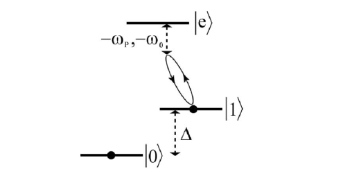
Figure 1: The three-state level structure of the atom or impurity complex. The two long-lived ground states $\left|0\right\rangle$ and $\left|1\right\rangle$ form the qubit and feature a large energy separation $\hbar\Delta$. Only the transition between state $\left|1\right\rangle$ and state $\left|{\rm e}\right\rangle$ is optically active. The optical pulse is detuned from this transition by $\omega_{{\rm\textsc{\scriptsize p}}}$ and the cavity mode is detuned by $\omega_{0}$.

Realistically, the fidelity of this operation is reduced by any leaked “which-path” information. This loss may be provided by light leaking from the fiber between the cavities, and it may be provided by a small probability for atomic absorption during the supposedly dispersive interaction. The former effect is unavoidable, and ultimately limits the fidelity of the post-selected entangled state to a value much lower than the theoretical expectations for most other proposals for cqed-based entanglement distribution [6, 7, 8, 9, 10, 11]. However, in this case the light used is bright and readily available from a laser source, the detection can be done with high efficiency, and the critical phase information can be stabilized by sending a trailing reference pulse down the same optical fiber. For these reasons, the expected fidelity, though low, is realistic with existing fiber-based technology, and the probability of successful post-selection of the desired state is very large, leading to a very fast initial entanglement distribution. If we then add a suitable protocol for nested entanglement purification and entanglement swapping [12], the low fidelity may be fairly quickly improved to near-unity values.

The generation of entanglement in our scheme is probabilistic but heralded, like a number of previous proposals. Deterministic cqed-based entanglement distribution schemes exist [6, 11], but such schemes put more challenging constraints on optical cavities and optical pulses. Duan et al [8] proposed a probabilistic scheme using Raman scattering from atomic ensembles. This scheme has recently seen an experimental implementation [13]. Integration of this system into a larger repeater architecture may be difficult; proposals operating on the principle of state-selective scattering from single emitters in cavities may be better suited for realistic implementations. Childress et al [9] have described a scheme in which such emitters reside in each path of an interferometer. Duan and Kimble [14] have proposed the use of the $\pi$-phase shift incurred upon reflection of a single photon from a loaded cavity as the basis for quantum logic [14], and a similar principle has been proposed for a quantum repeater design by Waks and Vuckovic [10], with an architecture consistent with photonic-crystal microcavities. In common to all of these schemes is a reliance on single photon (or sub-photon coherent state) transmission between the distant qubits. Although the heralded entanglement may have high initial fidelity, the high probability for channel loss means that the frequency of successful entangling events decreases exponentially with the distance between repeater stations. Since the rate of attempts is inevitably limited by the classical communication time between the distant stations, the use of single photons greatly reduces the speed of entanglement generation. The present scheme’s crucial difference is the use of bright pulses which assure successful post-selection for about 36% of the pulses sent down the channel. The trade-off for this increased speed is the limited fidelity of the post-selected entanglement, requiring additional entanglement purification.

For entanglement purification and swapping, local quantum logic is necessary. This step is especially challenging in proposals well suited to long-distance entanglement distribution, such as systems based on atomic ensembles [8]. If large and nearly absorption-free phase shifts are available, however, the same off-resonant interactions used for entanglement distribution may be used for a controlled-sign gate based on the geometrical phase [15]. This gate is measurement-free and completely deterministic, allowing rapid entanglement purification and swapping. However, it is far less robust to optical loss than the entanglement distribution scheme.

The final entanglement fidelity will depend on the fiber loss, certainly, but also on the amount of absorption in the dispersive interaction between the optical pulse and the emitter/cavity system. In this work we will show the physical criteria required for the desired qubit coherence to be well preserved even in the presence of this small but finite absorption. We will focus on systems in the intermediate coupling regime, or “bad cavity limit,” where the light-matter coupling is smaller than the rate of light-leakage from the cavity, but strong enough to substantially modify the rate of spontaneous emission. This regime is relevant for practical, homogeneous emitters in solid-state cavity systems.

We will begin in section 2 by considering how initial probability of success and fidelity affect the final rate of quantum communication; this discussion will show the potential advantage of the current proposal. Then section 3 will analyze the procedure for long-distance entanglement distribution and local quantum logic, in more detail than the sketch above or our previous treatment [5]. For this treatment the cqed interaction will be idealized. Once we have established the important figures of merit, we will estimate the ability for real cqed systems to implement this proposal. Our methods of analysis are explained in section 4, with results presented for three different regimes of operation in section 5.

2 Motivation: Final Rate of Communication after Entanglement Purification and Swapping

The means of distributing long-distance entanglement sketched in the introduction differs from most other proposals for heralded entanglement primarily in the fact that the probability of successful initial entanglement generation is high ($\sim 36\%$), while the initial fidelity is low ($\sim 77\%$). Before analyzing the origin of these numbers, let us address the question of whether such a scheme is useful. Obviously, an increase in the probability of success will increase the final rate of communication. However, the need for more entanglement purification will also slow down the final rate of communication. The question we address in this section is how the probability of success and fidelity affect the rate of final long-distance entanglement in a complete quantum repeater architecture.

2.1 Entanglement Purification and Swapping Protocol

The answer to this question depends on the protocols used for entanglement purification and entanglement swapping. Three such protocols for entanglement purification were presented in [12]. This important work analyzed the efficiency of “nested purification” schemes, in which imperfect distance-doubling entanglement swapping procedures are followed by entanglement purification. These schemes consider $N+1$ repeater stations (including end-stations), where $N=\mathcal{L}/\ell$, for total distance $\mathcal{L}$ subdivided into distances $\ell$ between adjacent stations. Very fast schemes (“A” and “B”) were considered in which hundreds of logically connected qubits are present in each station, as well as a scheme (“C”) in which as few as two qubits and at most $2\log_{2}N$ are present in the stations. More recent work [9] has shown that it can be sufficient to have only two qubits in every station. In these protocols the initial fidelity of entanglement distribution is considered to be quite high, so that purification is only used to correct for fidelity degradation and gate error during entanglement swapping.

Schemes using a minimal number of qubits are inevitably slow, since the initial entanglement generation and purification protocols are probabilistic, and with a minimal number of qubits, the entire protocol must begin from the start after each failure. A slow protocol cannot be remedied by arbitrarily speeding up the entanglement generation and purification procedures, since these are inevitably limited by the time it takes to transfer information between adjacent stations. The rate of final entanglement generation does speed up considerably if an ensemble of qubits is present in each station, as in schemes A and B of [12]. However, these schemes present an extreme case where arbitrarily many qubits are allowed in order to exponentially speed the purification process (the number needed grows polynomially with distance). As logically coupled qubits present an expensive resource, such schemes may be too expensive.

We consider instead a scheme similar to scheme B of [12], still using an ensemble of qubits, but we restrict the size of that ensemble as much as possible. From scheme C of [12], we know that at least $2\log_{2}N$ qubits are needed to allow the distance-doubling nested purification scheme to proceed in parallel to entanglement generation. If the initial fidelity begins low, so that entanglement of qubits in adjacent stations requires initial purification, two more qubits are needed in each section. Therefore at least $2+2\log_{2}N$ qubits are needed. To speed the protocol without increasing qubit overhead more than this, we consider putting $2+2\log_{2}N$ qubits in each of the repeater stations (including the endpoint receiver and sender). Initial entanglement is generated in parallel between the $1+\log_{2}N$ “send” qubits and the $1+\log_{2}N$ “receive” qubits in each station. This parallel operation significantly improves the speed of the initial entanglement generation, and allows simultaneous generation of new entangled pairs while long-distance pairs wait for purification.

With this number of qubits assumed, the protocol followed is straightforward. Each station purifies a certain number of steps as successful entanglement post-selections occur. Once the prescribed number of purification steps are done for both a send and a receive qubit in the same repeater station, Bell-state analysis is performed for entanglement swapping, assuring that each such process doubles the distance over which the qubits are entangled. After purification or swapping operations, each station immediately begins sending and receiving new optical pulses to and from any available qubit for further entanglement generation. The specific purification procedure we consider is similar to that used in scheme B of [12], the recurrence protocol originally presented in [16]. One slight modification which will be important for the specific entanglement scheme we discuss in later sections is that in each purification step, the local rotations performed before the controlled-not gates are chosen case-by-case to optimize the subsequent fidelity. This operation requires no additional complexity in the implementation as long as the form of the noise present in the system is known in advance.

2.2 Probability of Success vs. Initial Fidelity

With such a protocol established, we may now begin to compare the interplay between initial probability of success and initial fidelity. We numerically simulate the protocol described above for $N+1=129$ stations, assuming that all processes are limited only by a communication time of 50${\rm~{}}\mu{\rm s}$ between adjacent stations, corresponding to about $\ell=10{\rm~{}km}$ station-to-station distance and a total distance of 1280 km. Once an entangled pair is generated at 1280 km, a quantum bit is teleported across that distance. When the teleported bit arrives at the last repeater station, the simulation marks the time, resets the qubit participating in the teleportation, and continues to work on generating more entanglement. It takes some time for the first long-distance pair to be generated; it takes less time for subsequent pairs to be generated as there is already some entanglement in the system. The differences in arrival times of between 5 and 30 bits are averaged, and from this we obtain an average rate of long-distance quantum communication.

This rate is very fast in the unrealistic case that the initial fidelity is high and no gate errors are present. A more realistic rate must consider the possibility of imperfect entanglement and faulty gates. In this section we model error in a general way: we use a simple white-noise model for a two-qubit density operator, defined by

$$\rho\rightarrow(1-\epsilon)\rho+(\epsilon/4)\mathbf{1},$$ (1)

where $\mathbf{1}$ is the two-qubit identity matrix.

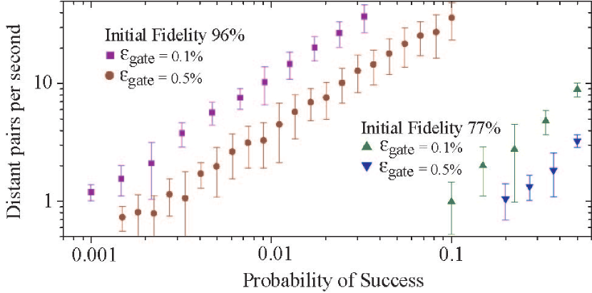
Figure 2: Final communication rate for a full nested purification protocol assuming an abstract white-noise process for the initial state generation and local gate error, with numbers of purification steps chosen to target a final fidelity of about 95%. The squares and circles, corresponding to an initial fidelity of 96%, show a final rate which varies slightly sublinearly with success probability ($\propto P^{0.93}$). The triangles correspond to an initial fidelity of 77% and show a slightly superlinear dependence ($\propto P^{1.2}$).

Figure 2 shows results of such simulations, in all cases with a number of purification steps at each distance chosen to yield a final communication fidelity of about 95%. We have considered two cases in generating this plot. The first models proposals based on single photon detection [8, 9, 10], where the initial fidelity is quite high. We have chosen that the initial state is a desired Bell state with white noise added at a level of $\epsilon=5\%$, resulting in an initial fidelity of 96%. This number is comparable to theoretical expectations, although it is much lower than fidelities observed in existing experiments [13]. In schemes such as these, the probability of success is limited by channel loss, the total efficiency of the photon detection, the scattering probabilities from the qubits to be entangled, and a factor of 1/2 from the post-selection probability. Taken together, these factors can easily result in a realistic probability of success less than 0.001. In contrast, we have also considered a model in which the initial fidelity is quite low, using $\epsilon=30\%$ resulting in $77\%$ fidelity, a number we will motivate in the next section. At equal probability-of-success, such a scheme is of course much slower. However, we will see that it allows a realistic probability of success on the order of $36\%$, which is far out-of-reach of proposals based on single photons. Figure 2 shows us that if we compare to probabilistic single-photon based schemes with probability of successful entanglement generation less than about 0.5%, the much higher probability of success of 36% present in our proposal results in a higher final communication rate, despite the need for additional purification.

The white-noise model used for entanglement generation and gate error in this analysis leads to slower purification rates than what may be possible in actual practice. This model is only used here to isolate the issue of probability-of-success and fidelity from other issues. In section 3.5, we will revisit this swapping and purification protocol using more realistic error models for our proposal, and we will see that the expected communication rates are somewhat faster than the results in figure 2.

3 Quantum Information Processing with Dispersive Light-Matter Interactions

In this section, we analyze the basic means of generating entanglement using dispersive cqed interactions with bright coherent light, including the dominant error modes.

3.1 Idealized System

The basic qubit in this scheme is formed by the two lower states of a three-state $\Lambda$-system, as shown in figure 1. The two metastable qubit states are labelled $\left|0\right\rangle$ and $\left|1\right\rangle$. We define the Pauli-$Z$ operator for the qubit as

$$Z=\left|0\right\rangle\!\!\left\langle 0\right|-\left|1\right\rangle\!\!\left\langle 1\right|.$$ (2)

Coherent transitions (rotations) between these two states are presumed to be possible through methods we will not discuss here, such as stimulated adiabatic Raman transitions [17] or spin-resonance techniques [18]. In this paper we focus on optical transitions between one of the ground states, $\left|1\right\rangle$, and some excited state, $\left|{\rm e}\right\rangle$, which may be short-lived. We define the optical raising and lowering operators as

$$\sigma^{+}=\left|{\rm e}\right\rangle\!\!\left\langle 1\right|,\quad\sigma^{-}=\left|1\right\rangle\!\!\left\langle{\rm e}\right|.$$ (3)

We presume that our light is completely ineffective at inducing transitions between $\left|0\right\rangle$ and $\left|{\rm e}\right\rangle$ either because $\left|{\rm e}\right\rangle$ is too far off-resonance, because of a prohibitive selection rule, or some combination of the two. One example of such a system is provided by a semiconductor donor-bound impurity, where the qubit states are provided by electron Zeeman sublevels and the excited state is provided by the lowest bound-exciton state. Other examples include the hyperfine structure of trapped ions. In this paper we will always refer to the matter qubit as an atom although it may be a semiconductor impurity or quantum dot comprised of many atoms.

In an ideal case, off-resonant light results in the effective Hamiltonian

$$\mathcal{H}=-JnZ/2,$$ (4)

where $n$ is the photon number operator. (An arbitrary state-independent optical phase term has been removed from this Hamiltonian). This Hamiltonian is not physically exact, but rather a desired result of a strictly dispersive atom-cavity interaction. Such a Hamiltonian is often assumed after the excited state $\left|{\rm e}\right\rangle$ is “adiabatically eliminated.”

To motivate the next section, in which a more detailed model appears, let us first explain our entanglement protocol as if we had a lossless channel. Qubit 1 would initially be rotated into state $(\left|0\right\rangle_{1}+\left|1\right\rangle_{1})/\sqrt{2}$. When a pulse of coherent light, which we call the “bus,” reflects off of the cavity containing the qubit, the interaction lasting time $\theta_{1}/J_{1}$ results in the unitary evolution operator

$$U_{1}=\exp(i\theta_{1}nZ_{1}/2).$$ (5)

After this interaction, the bus with initial coherent state amplitude $\alpha$ and the rotated qubit would be described by the state

$$U_{1}\frac{1}{\sqrt{2}}\bigl{[}\left|0\right\rangle_{1}+\left|1\right\rangle_{1}\bigr{]}\left|\alpha\right\rangle=\frac{1}{\sqrt{2}}\bigl{[}\bigl{|}0\bigr{\rangle}_{1}\bigl{|}\alpha e^{i\theta_{1}/2}\bigr{\rangle}+\bigl{|}1\bigr{\rangle}_{1}\bigl{|}\alpha e^{-i\theta_{1}/2}\bigr{\rangle}\bigr{]}.$$ (6)

After traveling the fictitious lossless channel, the bus would then undergo an identical interaction with a second qubit, which had been synchronously rotated into the same initial state as the first. The resulting selective phase shift by $\theta_{2}=\theta_{1}=\theta$ yields the state

$$\frac{1}{2}\bigl{[}\bigl{|}0\bigr{\rangle}_{1}\bigl{|}0\bigr{\rangle}_{2}\bigl{|}\alpha^{i\theta}\bigr{\rangle}+\bigl{(}\bigl{|}0\bigr{\rangle}_{1}\bigl{|}1\bigr{\rangle}_{2}+\bigl{|}1\bigr{\rangle}_{1}\bigl{|}0\bigr{\rangle}_{2}\bigr{)}\bigl{|}\alpha\bigr{\rangle}+\bigl{|}1\bigr{\rangle}_{1}\bigl{|}1\bigr{\rangle}_{2}\bigl{|}\alpha^{-i\theta}\bigr{\rangle}\bigr{]}.$$ (7)

If $\alpha$ is made infinitely large, the states $\left|\alpha\right\rangle$, $\bigl{|}\alpha e^{i\theta}\bigr{\rangle}$, and $\bigl{|}\alpha^{-i\theta}\bigr{\rangle}$ are orthogonal, so that they may be distinguished by some detection scheme such as homodyne detection. Employing such a scheme and keeping only those events in which the bus carries zero phase shift (state $\left|\alpha\right\rangle$), we post-select the qubits into the maximally entangled Bell-state

$$\left|\Psi^{+}\right\rangle=\frac{1}{\sqrt{2}}\bigl{[}\left|0\right\rangle_{1}\left|1\right\rangle_{2}+\left|1\right\rangle_{1}\left|0\right\rangle_{2}\bigr{]}.$$ (8)

This Bell-state could now be used for quantum teleportation.

Unfortunately, the situation is more complicated in the presence of channel loss. In this case noise is introduced during the transmission of the bus, requiring a density operator approach to describe the state. In order to keep the noise reasonable, a finite value of $\alpha$ must be taken. Then the phase shift of the light cannot be perfectly resolved, and so a more detailed look at the homodyne detection is needed. We pursue this analysis in the following sections.

3.2 Effective Interaction with Channel Loss

In order to generalize and allow for the introduction of noise, we write the state of qubit 1 as a general density matrix $\rho_{1}$, possibly already entangled to other qubits. Equation 6 may then be generalized to

$$U_{1}\left|\alpha\right\rangle\rho_{1}\left\langle\alpha\right|U_{1}^{\dagger}=\bigl{|}\beta_{1}(Z_{1})\bigr{\rangle}\rho_{1}\bigl{\langle}\beta_{1}(Z_{1})\bigr{|},$$ (9)

where

$$\beta_{1}(Z_{1})=\alpha e^{iZ_{1}\theta_{1}/2}.$$ (10)

To clarify the notation, $Z_{1}$ is the operator of equation (2) operating on $\rho_{1}$; the meaning of operators inside kets is unambiguous in the basis where these operators are diagonal.

In the state described by equation (9), the qubit may be highly entangled with the bus. The maximum degree of entanglement can be found from the entropy increase after tracing over the optical states; as $\alpha\rightarrow\infty$, this approaches $1-\exp(-4|\alpha|^{2}\sin^{2}\theta_{1}/2)$ bits, indicating that the entanglement increases as we increase the average photon number of the pulse $|\alpha|^{2}$. Unfortunately, in a real system, as $\alpha$ is increased so does the amount of quantum information leaked to the environment by various forms of loss. In order to estimate the amount of entanglement actually available from this interaction, we must address these non-idealities.

During the dispersive atom-cavity interaction, there is some probability that the atom is brought to state $\left|{\rm e}\right\rangle$, after which it may undergo spontaneous emission or undergo non-radiative decay. This probability leads to a very damaging decoherence, since a single spontaneously emitted photon, phonon, or Auger-ionized particle reveals the “which-path” information of the qubit. In the idealized picture governed by equation (4), such a form of loss is not present, but we will consider it in detail in ensuing sections, where we refer to such processes as internal loss.

For long-distance entanglement distribution, the dominant source of loss of photons is not from the cavity but rather from the ensuing communication channel. This loss depends on the length of the fiber connecting the cavities, although it may also be affected by imperfect mode-coupling to the cavity and the need to shift the wavelength of the cavity emission to a more convenient telecommunication wavelength [19, 20]. We refer to such processes as external loss.

For now, let us consider only the dominant source of loss: external loss from the fiber and associated mode coupling. In this case the bus coherent state is damped from $\left|\beta_{1}(Z_{1})\right\rangle$ to $\left|\sqrt{T}\beta_{1}(Z_{1})\right\rangle$, where $T$ is the total transmission from one cavity to the next. The lost photons are in principle lost into many modes. Although the physics of each loss mode may be complicated, we may treat it as we would a series of beam splitters. We write the lost photons in state

$$\left|L\right\rangle=\sum_{m}D_{m}(\alpha^{{\rm(L)}}_{m}e^{iZ_{1}\theta_{1}/2})\left|{\rm vacuum}\right\rangle,$$ (11)

where $D_{m}(\alpha^{{\rm(L)}}_{m})$ is the displacement operator for loss mode $m$, and the total power in these modes must sum to the total amount of lost optical power, $\sum_{m}|\alpha^{{\rm(L)}}_{m}|^{2}=(1-T)|\alpha|^{2}$. We may immediately trace over these modes. As a result of a single atom-cavity interaction followed by loss, the effective interaction accomplishes the quantum operation

$$\left|\alpha\right\rangle\rho_{1}\left\langle\alpha\right|\rightarrow\bigl{|}\sqrt{T}\beta_{1}(Z_{1})\bigr{\rangle}Q_{1}(\rho_{1})\bigl{\langle}\sqrt{T}\beta_{1}(Z_{1})\bigr{|}.$$ (12)

The superoperator $Q_{1}$ is given by a rotation and a phase flip with probability $\lambda_{-}$:

$$Q_{1}(\rho)=e^{iZ_{1}\xi_{1}/2}\bigl{[}\lambda_{+}\rho+\lambda_{-}Z_{1}\rho Z_{1}\bigr{]}e^{-iZ_{1}\xi_{1}/2}.$$ (13)

The parameters $\lambda_{\pm}$ are given by $(1\pm e^{-\gamma_{1}})/2.$ The losses $\gamma_{1}$ and phase shifts $\xi_{1}$ are given by

$$\gamma_{1} =|\alpha|^{2}(1-T)(1-\cos\theta_{1}),$$ (14)

$$\xi_{1} =|\alpha|^{2}(1-T)\sin\theta_{1}.$$ (15)

The rotation by angle $\xi_{1}$ can be quite large for realistic transmission $T,$ but such a single qubit operation may be undone locally. A key assumption here is that this phase is accurately known, which will require prior knowledge and stability of the angle $\theta_{1}$ and real-time measurement of $\alpha$ and $T$. The loss of coherence going as $\exp(-\gamma_{1})$ is the dominant and unavoidable source of the reduction of entanglement fidelity.

3.3 Long-Distance Entanglement Distribution

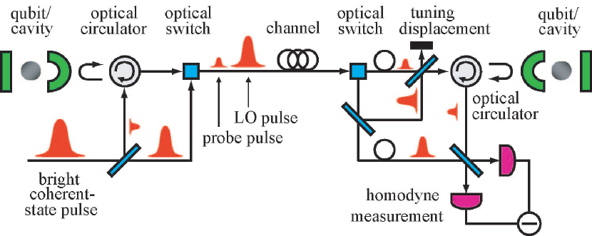
Figure 3: Schematic for long-distance entanglement distribution. A laser pulse is split into a local oscillator (lo) pulse and a probe pulse. The latter reflects from the left cavity, travels nearly concurrently with the lo pulse, and reflects from the right cavity. Homodyne detection is then performed to post-select the entanglement.

We now show how to use this semi-ideal interaction to distribute entanglement over long distances, referring to Fig. 3. The goal is to post-select a bus state that lacks “which-path” phase information from its two interactions with two qubits.

Unfortunately, the two qubits are likely to have slightly different interaction constants $J$. The qubits may be somewhat inhomogeneous, but even perfectly homogeneous qubits will give different angles. As we discuss in section 4, the angle depends on $\alpha$, which is reduced due to fiber loss, and on the pulse length, which is increased due to fiber dispersion. Such an angle difference may be compensated as follows. After reflection from the first cavity, the bus pulse and a local oscillator (lo) pulse are transmitted nearly simultaneously down a single fiber. Note that the lo pulse undergoes the same random phase shifts that the bus pulse may have accrued as it traveled the fiber. The lo pulse is then immediately split in order to accomplish a small displacement of the bus pulse prior to interacting with the second cavity. Such a displacement occurs by mixing the very strong lo pulse, with amplitude $\alpha_{{\rm\textsc{\scriptsize lo}}}$, with the bus pulse at a $1-x:x$ beam-splitter, where $x\ll 1$. One output of the beam-splitter gives the bus displaced by a term of order $x\alpha_{{\rm\textsc{\scriptsize lo}}}$, while the decoherence caused by the light dumped at the other output is of order $x^{2}\alpha_{{\rm\textsc{\scriptsize lo}}}$, a term which adds to the external losses already discussed. Now, the displaced bus pulse interacts with the second cavity and qubit, this time resulting in phase $\pm\theta_{2}$ for each eigenvalue of the $Z_{2}$ operator acting on the state of the second qubit, $\rho_{2}$. This displacement and interaction yield the state

$$\eqalign{U_{2}D(\beta_{{\rm\textsc{\scriptsize t}}})\bigl{|}\sqrt{T}\beta_{1}(Z_{1})\bigr{\rangle}Q_{1}(\rho_{1})\otimes\rho_{2}\bigl{\langle}\sqrt{T}\beta_{1}(Z_{1})\bigr{|}D^{\dagger}(\beta_{{\rm\textsc{\scriptsize t}}})U_{2}^{\dagger}=\cr\qquad e^{i\phi_{{\rm\textsc{\scriptsize t}}}(Z_{1})}\bigl{|}R+iI\bigr{\rangle}Q_{1}(\rho_{1})\otimes\rho_{2}\bigl{\langle}R+iI\bigr{|}e^{-i\phi_{{\rm\textsc{\scriptsize t}}}(Z_{1})},}$$ (16)

where

$$R+iI =\beta_{{\rm\textsc{\scriptsize t}}}e^{iZ_{2}\theta_{2}/2}+\sqrt{T}\alpha e^{i(Z_{2}\theta_{2}+Z_{1}\theta_{1})/2},$$ (17)

$$\phi_{{\rm\textsc{\scriptsize t}}}(Z_{1}) ={\rm Im}\{\sqrt{T}\alpha e^{-iZ_{1}/\theta_{2}}\beta_{{\rm\textsc{\scriptsize t}}}\}.$$ (18)

The ideal choice for the “tuning-displacement” amplitude $\beta_{{\rm\textsc{\scriptsize t}}}\approx x\alpha_{{\rm\textsc{\scriptsize lo}}}$ is

$$\beta_{{\rm\textsc{\scriptsize t}}}=\sqrt{T}\alpha\frac{\sin(\theta_{1}-\theta_{2})/2}{\sin\theta_{2}/2}.$$ (19)

With this choice, we find

$$R(Z_{1},Z_{2}) =\sqrt{T}\alpha\sin\frac{\theta_{1}}{2}\sin\frac{\theta_{2}}{2}\biggl{(}\cot^{2}\frac{\theta_{2}}{2}-Z_{1}Z_{2}\biggr{)},$$ (20)

$$I(Z_{1},Z_{2}) =\sqrt{T}\alpha\sin\frac{\theta_{1}}{2}\cos\frac{\theta_{2}}{2}(Z_{1}+Z_{2}).$$ (21)

The term $\exp[i\phi_{{\rm\textsc{\scriptsize t}}}(Z_{1})]$ represents a $Z$-rotation of qubit 1 by angle $-|\sqrt{T}\alpha|^{2}\sin(\theta_{1}/2-\theta_{2}/2)\sin(\theta_{1}/2)/\sin(\theta_{2}/2)$. Like the rotation by $\xi_{1}$ discussed in the last section, this large single qubit rotation may be removed, and so we will consider it no further.

To generate entanglement, we note that $I=0$ in the subspace where $Z_{1}+Z_{2}$ has eigenvalue 0. If the initial state of the qubits is $(\left|0\right\rangle_{1}+\left|1\right\rangle_{1})\otimes(\left|0\right\rangle_{2}+\left|1\right\rangle_{2})/2$, which is achieved by simultaneous, phase-coherent $\pi/2$ $Y$-rotations of the two distant qubits, and if we project onto the $Z_{1}+Z_{2}=0$ subspace, we achieve the maximally entangled Bell state $\left|\Psi^{+}\right\rangle$. Such a projection can be achieved by measuring a phase of zero from the bus state. In a probabilistic picture, this phase shift of zero implies one and only one of the atoms interacted with the pulse, but without information as to which atom caused the interaction, the quantum state is described by a superposition of both possibilities.

Of course, the phase of the pulse is a continuous quantum variable, and it may only be weakly post-selected with finite probability. Such weak post-selection may be accomplished by $p$-homodyne detection, in which we interfere the bus state with a lo pulse $\pi/2$ out of phase from the initial bus pulse . The difference photon number in the two output ports is measured; the result is proportional to the projected eigenvalue of $p=(a-a^{\dagger})/2i$ . As a result of this measurement, the qubits are projected into state

$$\bigl{\langle}p\!\bigm{|}\!R+iI\bigr{\rangle}Q_{1}(\rho_{1})\otimes\rho_{2}\bigl{\langle}R+iI\!\bigm{|}\!p\bigr{\rangle}=U(p)G(p)Q_{1}(\rho_{1})\otimes\rho_{2}G(p)U^{\dagger}(p),$$ (22)

where

$$U(p) =\exp[-i(2p+I)R],$$ (23)

$$G(p) =({2}/{\pi})^{1/4}\exp[-(p+I)^{2}].$$ (24)

How close is this conditional state to the desired Bell state $\left|\Psi^{+}\right\rangle$? Since $(Z_{1}+Z_{2})\left|\Psi^{+}\right\rangle=0$ and $Z_{1}Z_{2}\left|\Psi^{+}\right\rangle=-\left|\Psi^{+}\right\rangle$, we see that $\left|\Psi^{+}\right\rangle$ is an eigenstate of $U(p)$, and so $U(p)$ has no effect on the fidelity with respect to $\left|\Psi^{+}\right\rangle$. We therefore focus attention on the Gaussian projection operator $G(p)$. The projection described by this operator may be understood graphically in figure 4.

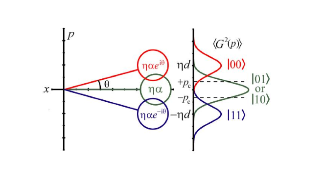
Figure 4: A quasi-probability distribution function (e.g. Wigner function) is shown on the left. The $p$-homodyne measurement yields a probability distribution function $\langle G^{2}(p)\rangle,$ shown on the right, found by integrating the Wigner function over $x$. The expectation value is evaluated for different choices of qubit states. The Gaussian peaks corresponding to finding the two qubits in states $\left|00\right\rangle$ or $\left|11\right\rangle$ are displaced from the $p=0$ origin by $\pm\sqrt{T}d$ due to the state dependent phase-shifts totalling to $\pm\theta$ that accrue during the interaction. However, states $\left|01\right\rangle$ and $\left|10\right\rangle$ accrue no total phase shift at the end, so if $p$ is measured between $-p_{{\rm c}}$ and $p_{{\rm c}}$, this subspace is approximately post-selected.

From this picture we see that any measurement with result near $p\approx 0$ projects the density operator into the parity-odd $Z_{1}+Z_{2}=0$ subspace. To post-select these cases, we keep only measurement results where $-p_{{\rm c}}<p<p_{{\rm c}}$. The probability of such an event is

$$\eqalign{P_{{\rm s}}&=\int_{-p_{{\rm c}}}^{p_{{\rm c}}}dp\ \Tr\{G^{2}(p)Q_{1}(\rho_{1})\otimes\rho_{2}\}\\ &=\frac{2\ {\rm erf}[\sqrt{2}p_{{\rm c}}]+{\rm erf}[\sqrt{2}(p_{{\rm c}}+\sqrt{T}d)]+{\rm erf}[\sqrt{2}(p_{{\rm c}}-\sqrt{T}d)]}{4}.}$$ (25)

Here we have used the important parameter

$$d=2\alpha\sin(\theta_{1}/2)\cos(\theta_{2}/2),$$ (26)

which we refer to as the distinguishability. Note that if $\theta_{1}=\theta_{2}=\theta,$ then $d=\alpha\sin\theta$. The fidelity of the post-selected state varies depending on the measurement result $p$. If we discard the information of the precise value of $p$ and automatically keep only those instances where $p$ falls in the post-selection window $|p|<p_{{\rm c}}$, the resulting density operator is calculated as an average of possibilities,

$$\rho_{12}^{{\rm\textsc{a}}}=\frac{1}{P_{{\rm s}}}\int_{-p_{{\rm c}}}^{p_{{\rm c}}}dp\ U(p)G(p)Q_{1}(\rho_{1})\otimes\rho_{2}G(p)U^{\dagger}(p).$$ (27)

The fidelity with respect to $\left|\Psi^{+}\right\rangle$ is then

$$F =\left\langle\Psi^{+}\right|\rho_{12}^{{\rm\textsc{a}}}\left|\Psi^{+}\right\rangle$$

$$=\frac{(1+e^{-\gamma_{1}}){\rm erf}[\sqrt{2}p_{{\rm c}}]}{2\ {\rm erf}[\sqrt{2}p_{{\rm c}}]+{\rm erf}[\sqrt{2}(p_{{\rm c}}+\sqrt{T}d)]+{\rm erf}[\sqrt{2}(p_{{\rm c}}-\sqrt{T}d)]}.$$

If $d\rightarrow\infty$, then the postselection operation $G(p)$ works very well, and $\rho_{12}^{{\rm\textsc{a}}}$ is entirely contained in the desired $Z_{1}+Z_{2}=0$ subspace. However, the fidelity reduction due to fiber loss is characterized by $\gamma_{1}=d^{2}(1-T)/2$ in the low $\theta$ limit. As $d\rightarrow\infty$, then, the $Q_{1}$ super-operator casts the two-qubit density operator into a classical superposition of $\left|01\right\rangle$ and $\left|10\right\rangle$, rather than the desired $\left|\Psi^{+}\right\rangle$ state. For quantum coherence to be preserved, $d$ must not be made too large.

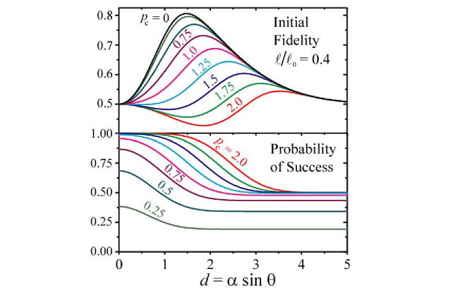
Figure 5: The top figure shows the fidelity with respect to Bell state $|\Psi^{+}\rangle$ as a function of distinguishability $d$ for linearly varying values of the post-selection measurement window parameter $p_{{\rm c}}$ between 0 and 2.0. The bottom figure shows the corresponding probability of success. The calculation assumes $T=0.67,$ corresponding to 10 km of telecom fiber and $\theta_{1}=\theta_{2}\ll 1$.

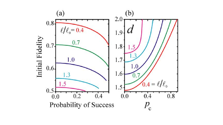
Figure 6: (a) Initial entanglement fidelity $F=\langle\Psi^{+}|\rho_{12}|\Psi^{+}\rangle$ vs. probability of success. Each curve is labeled by the distance between qubits, $\ell$, normalized by the attenuation length of the fiber, $\ell_{0}$. The probability of success is increased by increasing the post-selection window parameter $p_{{\rm c}}$, and $d$ is chosen for each $p_{{\rm c}}$ to maximize the fidelity. (b) The values of the distinguishability $d$ and post-selection window parameter $p_{{\rm c}}$ which lead to the maximum fidelities of subfigure (a).

Figure 5 shows the fidelity of the final two-qubit entanglement as a function of the distinguishability $d$ and the post-selection window for $T=0.67$. We see that at each $p_{{\rm c}}$, there is a maximum fidelity at which $d$ is large enough to allow good post-selection but not so large that fiber loss destroys all coherence. This maximum fidelity is largest at $p_{{\rm c}}=0$, but this condition means that the scheme would succeed an infinitesimal number of times. At larger values of $p_{{\rm c}}$ the probability of success increases, but since states outside of the desired $\left|\Psi^{+}\right\rangle$ state become more probable the optimal fidelity decreases somewhat. This optimal fidelity as a function of the probability of success is shown in figure 6(a), for several different possibilities of fiber length. The range of distinguishability $d$ required to achieve these curves is shown in figure 6(b). The calculations leading to these curves assume that $\theta\ll 1$, in which case the results depend to a good approximation only on $d$ and not independently on $\alpha$ or $\theta$.

In figure 6, the fiber length between repeater stations, $\ell$, is measured in units of the attenuation length $\ell_{0}$ [i.e. $T=\exp(-\ell/\ell_{0})$]. For fused-silica fibers at telecommunication wavelengths, the attenuation length $\ell_{0}$ can be as high as 25 km. It is clear that much higher fidelities are available for communication distances much shorter than this length, but then the spacing of repeater stations may be too small to be practical. For longer distances, the reduced fidelity will require more purification . Optimizing the distance between repeater stations will involve a large number of trade-offs, and the best choice will depend on the efficiency of the purification protocol.

As an example, a typical working condition is $\ell/\ell_{0}\approx 0.4$, corresponding to 10 km of fiber and $T$=0.67; these choices were used for figure 5. If we choose $p_{{\rm c}}=0.5$, the probability of success is 36% and the initial fidelity is 77%. Since the light source can be a normal stabilized laser and detection is extremely efficient, this 36% probability of success is not degraded by source or detector efficiency. The rate of initial entanglement generation is therefore extremely fast in comparison to most other schemes for entanglement distribution.

3.4 The Measurement-Free C-$Z$ Gate

The rate of final, long distance entanglement will depend on the efficiency of the protocol for entanglement purification and swapping [12], which depends on the fidelity of local operations (especially two-qubit gates such as controlled-not). A complete architecture for a quantum repeater requires some way of achieving these local operations.

The entanglement distribution scheme discussed in the previous section could in principle be used for these local operations, but its probabilistic nature leads to very inefficient purification protocols. Deterministic local operations not involving post-selection are possible using the same resources we have already assumed for entanglement distribution, i.e. the effective interaction of equation (4) with $d\sim 1$. Ways to achieve quantum logic gates with these resources were discussed in [15]. One method uses this effective interaction to approximate controlled displacements, and employs the Berry-phase accumulation under those displacements to achieve a controlled-sign (C-$Z$) gate. The specific choice of operations to construct the gate is as follows. The gate occurs between two qubits, each in separate cavities connected by a short, local waveguide network. First, a dispersive interaction with qubit 1 is performed, as described in section 3.2. Then the optical bus in state $\left|\beta_{1}(Z_{1})\right\rangle$ is mixed with a lo pulse at a beamsplitter with amplitude and phase chosen to achieve a displacement of $\alpha(i-1)$. Following this displacement, an effective interaction between the bus and qubit 2 is performed. The bus state may now be described as $\left|\beta_{2}(Z_{1},Z_{2})\right\rangle,$ where

$$\beta_{2}(Z_{1},Z_{2})=e^{iZ_{2}\theta_{2}/2}\bigl{[}\beta_{1}(Z_{1})+(i-1)\alpha_{1}\bigr{]}.$$ (29)

We have written $\theta_{2}$ for this second interaction in case the controlled rotation during this interaction is slightly different from the first. After this interaction, the bus is again displaced, this time by $-\alpha(1+i)$, after which it interacts with the first qubit again. This brings the optical bus to state $\left|\beta_{3}\right\rangle$, where

$$\beta_{3}(Z_{1},Z_{2})=e^{iZ_{1}\theta_{3}/2}\bigl{[}\beta_{2}(Z_{1},Z_{2})-(i+1)\alpha_{2}\bigr{]}.$$ (30)

The cycle is completed by a displacement by $\alpha(1-i)$ and a final interaction with the second qubit, resulting in state $\left|\beta_{4}\right\rangle,$ where

$$\beta_{4}(Z_{1},Z_{2})=e^{iZ_{2}\theta_{4}/2}\bigl{[}\beta_{3}(Z_{1},Z_{2})-(i-1)\alpha_{3}\bigr{]}.$$ (31)

If $\theta_{n}$ is the same for every interaction, then this final coherent state amplitude is approximately a constant term, $-i|\alpha|^{2}$, plus a term proportional to $d^{2}$ involving the product operator $Z_{1}Z_{2}$. (If $\theta_{n}$ differs during each interaction, the gate requires modifications of the displacements to compensate, similar to the “tuning-displacement” used in the previous section.) The C-$Z$ gate results from the phase accrued when tracing over the bus state, in addition to the phases that accrued during the displacement. The final state-dependent phase contains terms proportional to $Z_{1}$ and $Z_{2}$, which correspond to single qubit rotations, but also the term $|\alpha\theta|^{2}Z_{1}Z_{2}/2$, for small $\theta$. With the bus state removed and single qubit rotations corrected, this remnant phase is a nonlocal unitary operator acting on the two qubits, which may be used as a C-$Z$ gate if $|\alpha\theta|^{2}=\pi/2$. More details of this calculation, including the effects of optical loss, may be found in A.

As in the scheme for entanglement distribution, the performance of this C-$Z$ gate is limited by both internal cavity losses and external losses. As this is a local gate, these external losses are dominated by the interfaces between short waveguides and the required cavities and beamsplitters.

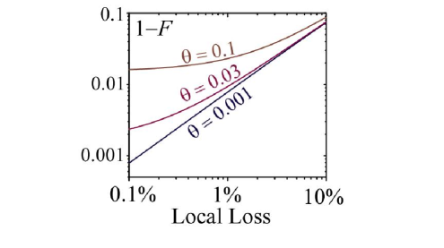
Figure 7: This shows $1-F$, where $F=\lambda_{0}$ is the fidelity of the measurement-free C-$Z$ gate, as a function of the local external optical loss, for several different values of $\theta$, maintaining the requirement $\alpha\theta\sim 1$. See A.

The total fidelity of each gate as a function of local, external loss is shown in figure 7. This fidelity reduction should be compared to the error due to internal loss. The C-$Z$ gate we analyzed interacts with each of the two qubits twice, and therefore the total error due to internal losses goes as the calculated fidelity of the atom-cavity interaction to the fourth power. Whether internal or external losses will dominate for this gate will depend heavily on the details of the system used to implement it.

3.5 Final Communication Rate

To estimate the final communication rate for this proposal, we revisit the entanglement purification and swapping protocol discussed in section 2. We repeat the same simulation, except using more realistic noise models. We use the calculated initial density matrix given by equation (27) for the initial state, estimating that external loss is dominated by the attenuation length of standard fused silica fiber at telecom wavelength. We use the noise model developed in A to model gate errors during entanglement purification and entanglement swapping; this noise is dominated by local loss in the short waveguides between qubits in a single repeater station. We assume perfect single-spin rotations. As an illustratitve example, we again presume $N+1=129$ repeater stations, each spaced by 10 km, with $2+2\log_{2}N=16$ qubits in each station. Each qubit is in its own cavity. Such an architecture could be implemented using fiber-optic waveguides and switches, or on a single chip using planar photonic crystal waveguides and switches.

A typical number of purification steps under these conditions might be three rounds of entanglement purification of nearest-neighbor, initially generated entanglement, two rounds of entanglement purification after the first few levels of entanglement swapping, and one or zero steps of entanglement swapping for the last few levels of highest-distance entanglement swapping. The exact number of steps is varied from simulation to simulation to achieve different communication rates and different levels of final fidelity. Figure 8 shows the final communication rate and fidelity for several example choices as a function of local external optical loss. Communication rates approaching 100 Hz appear to be possible.

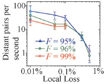
Figure 8: Rates of final generation of distant (1280 km) entangled pairs resulting from Monte-Carlo simulations of the nested entanglement protocol with 16 qubits per station and 127 intermediate stations separated by 10 km. The simulations run until 5 pairs are generated; the average time and standard deviation between generated pairs is plotted. The error modes included in the simulation are the initial fidelity reduction due to external loss in the 10 km fiber and distortion due to local external losses during the measurement-free C-$Z$ gate, as described in A. Different numbers of purification steps are used to achieve different final fidelities.

4 Calculation of the Dispersive Light-Matter Interaction: Methods

Up until now, we have assumed the effective Hamiltonian of equation (4), and we have argued that this is a sufficient interaction to achieve a fast, long distance quantum communication protocol. Unfortunately, the idealized interaction described by equation (4) is not physically available in a cqed system, except as an approximation. This approximation assumes the “bounce” fidelity of the dispersive interaction is negligibly close to one. In this section, we analyze the physical parameters of the atom-cavity system required to satisfy this assumption.

Most existing theoretical analyses of cqed designs for entanglement generation are only appropriate in regimes different from those considered here. For the strongly coupled regime, evaluation of dynamics in a dressed-state picture is an effective means of calculation, but in the weak or intermediate coupling regime, the large widths of the dressed states make such calculation techniques inappropriate. Weak-coupling or intermediate-coupling calculations usually make one of several approximations. One simplifying assumption is that only single photons or weak-coherent states interact with the cavity, heavily limiting the dimensionality of the equations to be solved. This has been effective for studies of spontaneous emission and the proposals for cqed devices in the weak-excitation limit, but it will not be effective here. Typically, when more photons are introduced into the cavity, a numeric approach is required. For very large photon numbers, a full-quantum analysis can be computationally intensive; an appropriate approximation is the semi-classical optical Bloch equation approach. We will primarily work under such assumptions in the present study.

We establish notation by first describing and solving the empty cavity problem. We then compare the interaction in a loaded cavity using an interaction picture that only considers dynamics in a frame with the empty-cavity dynamics removed. We begin with an analytic, perturbative approach, which expands the dynamics in the atom-cavity coupling $g$ and the bare-atom relaxation rate $\tau^{-1}$. These are presumed to be much smaller than the time for light to leak out of the cavity, $\omega_{0}/Q$ (weak or intermediate coupling regime.) It is not assumed that the atom is never excited, or that the photon number is small, although we will see that the expansion fails if the photon number is large enough to saturate the interaction. For more accurate results, we will employ a semi-classical simulation of the full many-photon atom-cavity dynamics. We will check the results of this semi-classical approach against the results of the perturbative calculation in the low photon number regime and against a fully quantum analysis in the high photon number regime.

4.1 Empty Cavity

The empty-cavity Hamiltonian is

$$\mathcal{H}_{{\rm 0}}=\omega_{0}a_{0}^{\dagger}a_{0}^{\phantom{{\dagger}}}+\sum_{\lambda}\omega_{\lambda}b_{\lambda}^{\dagger}b_{\lambda}^{\phantom{{\dagger}}}+i\sum_{\lambda}\kappa_{\lambda}(b_{\lambda}^{\phantom{{\dagger}}}a_{0}^{\dagger}-b_{\lambda}^{\dagger}a_{0}^{\phantom{{\dagger}}}).$$ (32)

We are working in a frame rotating at the frequency of the $\left|{\rm e}\right\rangle\leftrightarrow\left|1\right\rangle$ transition, $\omega_{{\rm a}}$. The operators $b_{\lambda}$ ($b_{\lambda}^{\dagger}$) annihilate (create) photons in the eigenstates of the waveguide to the cavity, with eigenenergies $\hbar(\omega_{{\rm a}}+\omega_{\lambda})$. The cavity-waveguide coupling constants $\kappa_{\lambda}$ are assumed to be real. The sum includes lossy modes and absorptive losses in the cavity mirrors. The operators $a_{0}$ and $a_{0}^{\dagger}$ respectively annihilate and create photons in the single cavity mode. We further make a transformation to wave-packet modes

$$a_{m}^{\dagger}=\sum_{\lambda}b^{\dagger}_{\lambda}u_{\lambda m}^{\phantom{{\dagger}}},$$ (33)

for $m>0$, where $u_{\lambda m}$ is a unitary matrix. (When summing over modes in the following formalism, the $m=0$ cavity mode is also included.) The element $u_{\lambda m}$ is the Fourier component of a traveling pulse with label $m$. Two modes are of particular interest: $a_{\rm\textsc{\scriptsize in}}$ annihilates a photon in the wavepacket incident on the cavity, and $a_{\rm\textsc{\scriptsize out}}$ annihilates a photon in the wavepacket of the output mode which couples to the waveguide for communication. Hence $u_{\lambda,{\rm\textsc{\scriptsize in}}}$ describes the input pulse shape $f_{\rm\textsc{\scriptsize in}}(\vec{r},t)$ according to

$$u_{\lambda,{\rm\textsc{\scriptsize in}}}=\int_{V}d^{3}\vec{r}\int_{-\infty}^{\infty}dt\ \psi^{*}_{\lambda}(\vec{r})e^{i\omega_{\lambda}t}f_{\rm\textsc{\scriptsize in}}(\vec{r},t),$$ (34)

where $\psi_{\lambda}(\vec{r})$ is the spatial shape of the wavepacket for waveguide eigenmode $\lambda$.

The solution of the empty cavity problem is well known; here we treat it as a scattering matrix for the operators $a_{m}$. The Heisenberg equations of motion are

$$\dot{a}_{0}(t) =-i\omega_{0}a_{0}(t)+\sum_{\lambda}\kappa_{\lambda}b_{\lambda}(t),$$ (35a)

$$\dot{b}_{\lambda}(t) =-i\omega_{\lambda}b_{\lambda}(t)-\kappa_{\lambda}a_{0}(t).$$ (35b)

Using Laplace transforms, $a(s)=\int_{0}^{\infty}e^{-st}a(t)$, we arrive at the scattering matrix equation

$$b_{\lambda}(s)=\sum_{m}S_{\lambda m}(s)a_{m},$$ (35aj)

where

$$S_{00}(s) =\frac{1}{s+i\omega_{0}+\gamma/2},$$ (35aka)

$$S_{\lambda 0}(s) =-S_{00}(s)\frac{\kappa_{\lambda}}{s+i\omega_{\lambda}},$$ (35akb)

$$S_{0m}(s) =-\sum_{\lambda}S_{\lambda 0}(s)u_{\lambda m},$$ (35akc)

$$S_{\lambda m}(s) =\frac{u_{\lambda m}-\kappa_{\lambda}S_{0m}(s)}{s+i\omega_{\lambda}}.$$ (35akd)

We assumed a sufficiently broadband spectrum of output coupling and absorption modes to lead to an exponential cavity decay function [23]; this came from the mathematical association

$$\sum_{\lambda}\frac{\kappa^{2}_{\lambda}}{s+i\omega_{\lambda}}=\frac{\gamma}{2},$$ (35akal)

implying that any optical power in the cavity leaks out of the cavity as $e^{-\gamma t}$.

We also introduce an average output coupling factor $\kappa$ (without subscript) as follows. Suppose at $t=0$ the cavity contains a single photon, $\left|\psi(0)\right\rangle=a_{0}^{\dagger}\left|0\right\rangle$. Then after some time the photon leaks into all possible modes $\lambda$,

$$\lim_{t\rightarrow\infty}\left|\psi(t)\right\rangle=\lim_{t\rightarrow\infty}\sum_{\lambda}S^{\dagger}_{0\lambda}(t)b^{\dagger}_{\lambda}\left|0\right\rangle.$$ (35akam)

Many of the modes indexed by $\lambda$ will not be included in the desired output wavepacket. We therefore seek the overlap of this state with that of a single photon in the input mode, $\left|\phi_{\rm\textsc{\scriptsize in}}(t)\right\rangle=\sum_{\lambda}e^{-i\omega_{\lambda}t}b_{\lambda}^{\dagger}u_{\lambda,{\rm\textsc{\scriptsize in}}}\left|0\right\rangle$ in the limit where $t\rightarrow\infty$. We arrive at the overlap integral

$$\bigl{\langle}\psi(t)\!\bigm{|}\!\phi_{\rm\textsc{\scriptsize in}}(t)\bigr{\rangle}=\sum_{\lambda}\frac{\kappa_{\lambda}u_{\lambda,{\rm\textsc{\scriptsize in}}}}{i(\omega_{\lambda}-\omega_{0})-\gamma/2}\equiv\sqrt{\kappa}F_{\rm\textsc{\scriptsize in}}^{\phantom{*}}\bigl{(}-i\omega_{0}-{\gamma}/{2}\bigr{)}.$$ (35akan)

where $F_{\rm\textsc{\scriptsize in}}(s)$ is the Laplace transform of the input pulse shape for mode $m$ as it couples into the cavity. Two effects are present in this overlap: first there is the overlap of the pulse transform with the cavity filter function, indicated by the Laplace transform of the input light $F_{\rm\textsc{\scriptsize in}}(s)$ at $s=-i\omega_{0}-\gamma/2$. Second, there is the output coupling factor $\kappa$; only a fraction of roughly $\kappa/\gamma$ of the light makes it from the cavity to the output mode.

Using these definitions, we write

$$S_{0,{\rm\textsc{\scriptsize in}}}(s)=\sqrt{\kappa}\frac{F_{\rm\textsc{\scriptsize in}}(s)}{s+i\omega_{0}+\gamma/2}.$$ (35akao)

This function, which represents the convolution of the input pulse with the filter function of the cavity, will be used heavily in what follows. The pulse reflected from the cavity can be seen from equations (35akao) and (35akd) to have components

$$S_{\lambda,{\rm\textsc{\scriptsize in}}}(s)=\frac{1}{s+i\omega_{\lambda}}\biggl{[}u_{\lambda,{\rm\textsc{\scriptsize in}}}-\frac{\kappa_{\lambda}}{s+i\omega_{0}+\gamma/2}\sqrt{\kappa}F_{\rm\textsc{\scriptsize in}}(s)\biggr{]},$$ (35akap)

and therefore

$$\sum_{\lambda}u_{{\rm\textsc{\scriptsize in}},\lambda}^{\dagger}S_{\lambda,{\rm\textsc{\scriptsize in}}}^{\phantom{{\dagger}}}(s)=\frac{|u_{\lambda,{\rm\textsc{\scriptsize in}}}|^{2}}{s+i\omega_{\lambda}}-\frac{\kappa}{s+i\omega_{0}+\gamma/2}|F_{{\rm\textsc{\scriptsize in}}}(s)|^{2}.$$ (35akaq)

The first term describes the traveling wave corresponding to mode in, the second term describes the interference from light that coupled in and then back out of the cavity. If the cavity mirror passed all modes with equal coupling, then the light entering the cavity would have the same shape as the input pulse, i.e. $|F_{\rm\textsc{\scriptsize in}}(p)|^{2}=\sum_{\lambda}|u_{\lambda,{\rm\textsc{\scriptsize in}}}|^{2}/(p+i\omega_{\lambda})$. In this limit, we would have

$$\sum_{\lambda}u_{{\rm\textsc{\scriptsize in}},\lambda}^{\dagger}S_{\lambda,{\rm\textsc{\scriptsize in}}}^{\phantom{{\dagger}}}(s)=\sum_{\lambda}\frac{|u_{\lambda,{\rm\textsc{\scriptsize in}}}|^{2}}{s+i\omega_{\lambda}}\biggl{[}\frac{s+i\omega_{0}+\gamma/2-\kappa}{s+i\omega_{0}+\gamma/2}\biggr{]}.$$ (35akar)

If we further assume the cavity to be strongly overcoupled ($\kappa=\gamma$), we arrive at the solution for reflection from an empty cavity found in [23].

The empty cavity is a linear scattering problem and may be solved with this scattering matrix approach. However, the presence of an atom in the cavity transforms it to a nonlinear problem. For this we consider the characteristic function

$$\chi(\eta,t)=\Tr\{D_{\rm\textsc{\scriptsize out}}(\eta,t)\rho(t)\},$$ (35akas)

where $D_{\rm\textsc{\scriptsize out}}(\eta,t)$ is the displacement operator for the time-dependent output mode out:

$$D_{\rm\textsc{\scriptsize out}}(\eta,t)=\exp[\eta a^{\dagger}_{\rm\textsc{\scriptsize out}}(t)-\eta^{*}a^{\phantom{{\dagger}}}_{\rm\textsc{\scriptsize out}}(t)],$$ (35akat)

for $a_{\rm\textsc{\scriptsize out}}^{\dagger}(t)=\sum_{\lambda}b_{\lambda}^{\dagger}S_{\lambda,{\rm\textsc{\scriptsize in}}}^{\phantom{{\dagger}}}(t)$. If the input wave-packet is a coherent-state with amplitude $\alpha$ and the cavity is empty, we find

$$\chi_{0}(\eta,t)=e^{-|\eta|^{2}/2}\prod_{\lambda}\Tr\left\{e^{-\eta^{*}S_{{\rm\textsc{\scriptsize in}},\lambda}^{\dagger}(t)b_{\lambda}^{\phantom{{\dagger}}}}\bigl{|}S_{\lambda,{\rm\textsc{\scriptsize in}}}(t)\alpha\bigr{\rangle}\!\!\bigl{\langle}S_{\lambda,{\rm\textsc{\scriptsize in}}}(t)\alpha\bigr{|}_{\lambda}e^{\eta S_{\lambda,{\rm\textsc{\scriptsize in}}}^{\phantom{{\dagger}}}(t)b_{\lambda}^{\dagger}}\right\}.$$ (35akau)

Now, we may use the unitarity of the scattering matrix, i.e.

$$\sum_{\lambda}S^{\dagger}_{m,\lambda}(t)S^{\phantom{{\dagger}}}_{\lambda,{\rm\textsc{\scriptsize in}}}(t)=\delta_{m,{\rm\textsc{\scriptsize in}}},$$ (35akav)

to see that

$$\chi_{0}(\eta,t)=e^{-|\eta|^{2}/2+\eta\alpha^{*}-\eta^{*}\alpha},$$ (35akaw)

the characteristic function of a coherent state in traveling wavepacket-mode out.

4.2 Atom-Cavity Interactions in the Interaction Picture

If the cavity is not empty, the time-dependence of $\rho$ will be more complicated. In this case, we consider the density operator in the interaction picture,

$$\chi(\eta,t)=\Tr\{\tilde{D}_{\rm\textsc{\scriptsize out}}(\eta,t)\tilde{\rho}(t)\},$$ (35akax)

where

$$\tilde{\rho}(t)=e^{i\mathcal{H}_{{\rm 0}}t}\rho(t)e^{-i\mathcal{H}_{{\rm 0}}t}$$ (35akay)

and

$$\eqalign{\tilde{D}_{\rm\textsc{\scriptsize out}}(\eta,t)&=e^{i\mathcal{H}_{{\rm 0}}t}D_{\rm\textsc{\scriptsize out}}(\eta,t)e^{-i\mathcal{H}_{{\rm 0}}t}\\ &=\exp\biggl{(}-\frac{|\eta|^{2}}{2}+\sum_{\lambda}\eta b_{\lambda}^{\dagger}(t)S^{\phantom{*}}_{\lambda,{\rm\textsc{\scriptsize in}}}(t)-{\rm h.c.}\biggr{)}\\ &=\exp\biggl{(}-\frac{|\eta|^{2}}{2}+\sum_{m,\lambda}\eta a_{m}^{\dagger}S^{\dagger}_{m\lambda}(t)S^{\phantom{{\dagger}}}_{\lambda,{\rm\textsc{\scriptsize in}}}(t)-{\rm h.c.}\biggr{)}\\ &=e^{-|\eta|^{2}/2+\eta a_{{\rm\textsc{\scriptsize in}}}^{\dagger}-\eta^{*}a_{{\rm\textsc{\scriptsize in}}}^{\phantom{{\dagger}}}}=D_{{\rm\textsc{\scriptsize in}}}(\eta,0).}$$ (35akaz)

“H.c.” refers to Hermitian conjugate.

To analyze the effect of an atom in the cavity (which we call an atom, although it may be a quantum dot or impurity complex), we consider unitary dynamics governed by a Jaynes-Cummings term [23],

$$\mathcal{H}_{{\rm int}}=g(a_{0}^{\phantom{{\dagger}}}\sigma^{+}+a_{0}^{\dagger}\sigma^{-}),$$ (35akba)

as well as non-unitary atomic relaxation processes. In the interaction picture, this Hamiltonian becomes time-dependent:

$$\tilde{\mathcal{H}}_{{\rm int}}(t)=g\sum_{m}\bigl{[}S_{0m}^{\phantom{*}}(t)a_{m}^{\phantom{{\dagger}}}\sigma^{+}+a_{m}^{\dagger}S_{m0}^{\dagger}(t)\sigma^{-}\bigr{]}.$$ (35akbb)

We assume that relaxation is limited by lifetime effects, so that the full Liouville-von Neumann equation may be written

$$\frac{d\tilde{\rho}}{dt}=-i[\tilde{\mathcal{H}}_{{\rm int}}(t),\tilde{\rho}(t)]+\mathcal{L}[\tilde{\rho}(t)].$$ (35akbc)

The latter terms represent atomic relaxation at zero temperature. Considering a master equation approach, we use

$$\mathcal{L}[\tilde{\rho}(t)]=-\frac{1}{2\tau}\bigl{[}\sigma^{+}\sigma^{-}\tilde{\rho}(t)+\tilde{\rho}(t)\sigma^{+}\sigma^{-}-2\sigma^{-}\tilde{\rho}(t)\sigma^{+}\bigr{]}.$$ (35akbd)

Here, $\tau$ is the lifetime of the atom in the absence of the cavity, including both spontaneous emission and non-radiative decay, such as Auger decay of bound excitons in silicon. In principle, pure decoherence terms could be added to the above; however in the present study we neglect decoherence between the two ground states and assume the optically created coherences are strictly lifetime broadened.

As we will see, the most important parameter for quantifying the performance of a particular atom-cavity system is related to the Purcell factor

$$\mathcal{F}(\omega)=\frac{{\tau_{{\rm r}}\gamma}g^{2}}{\omega^{2}+\gamma^{2}/4},$$ (35akbe)

where $\tau_{{\rm r}}$ is the spontaneous emission lifetime outside of the cavity. We will be considering systems where the atom is far detuned from the cavity frequency, so that the Purcell effect is weak. However, the key parameter quantifying the suitability of an atom-cavity system for strong dispersive interactions with low absorption is

$$\Phi=\frac{\tau}{\tau_{{\rm r}}}\frac{\kappa}{\gamma}\mathcal{F}(0).$$ (35akbf)

This parameter is sometimes known as the “cooperativity parameter” or the inverse of the “critical atom number.” We will see that if $\alpha$, the center frequency of the pulse, and the pulse width are optimally chosen, the final fidelity of the dispersive interaction approximately decreases as $\exp(-d^{2}/\Phi)$, so a large $\Phi$ is critical for high-fidelity operation.

We now have enough formalism to clarify a terminology we have already employed. We say that a cavity is in the strong coupling regime if $g>\gamma$ and $g>1/\tau$. The strong coupling regime is not optimal for this quantum repeater architecture. The optimal regime is the intermediate coupling regime; specifically this means that $g<\gamma$ but $\Phi>1$.

We estimate the atom-cavity coupling from the formula

$$g^{2}=\frac{3}{(4\pi)^{2}}\frac{\omega_{{\rm a}}}{\tau_{{\rm r}}}\frac{\lambda^{3}}{n^{3}V},$$ (35akbg)

where $V$ is the mode volume, $\tau_{{\rm r}}$ is the strictly radiative lifetime, $\lambda$ and $\omega_{{\rm a}}$ are the wavelength and frequency of the atomic resonance, and $n$ is the index of refraction of the host material. This formula assumes an optimally aligned dipole at the antinode of the cavity field. We even apply this formula to silicon, where the indirect, phonon-mediated transitions are not simple electric dipole transitions. The slightly different probabilities for phonon absorption and emission means that the silicon system is not exactly described by the Jaynes-Cummings model, but these corrections are not expected to be important for modeling far off-resonant dynamics. Using equation (35akbg), then, and assuming a pulse resonant with the cavity, we have

$$\Phi=\frac{3}{4\pi^{2}}\times\frac{\kappa}{\gamma}\times\frac{\tau}{\tau_{{\rm r}}}\times\frac{\lambda^{3}}{n^{3}V}\times Q.$$ (35akbh)

The four terms of this expression will serve to summarize the importance of each physical parameter. The factor $\kappa/\gamma$ indicates the degree that light leaking from the cavity leaks into the desired output mode. For the present quantum repeater application, it is best that the cavity is overcoupled; i.e. that cavity loss is dominated by transmission through the output mirror, so that $\kappa/\gamma\rightarrow 1$. The factor $\tau/\tau_{{\rm r}}$ is the ratio of the total lifetime of the atom divided by the radiative lifetime, i.e. the internal quantum efficiency of the emitter. This factor is detrimental in the case of donor-bound excitons in silicon, for example, where $\tau$ is dominated by Auger recombination. The factor $\lambda^{3}/n^{3}V$ indicates the importance of a microcavity in achieving a high value of $\Phi$. Finally, the total cavity $Q=\omega_{{\rm a}}/\gamma$ is a critical parameter; it must be large enough to compensate for deficiencies in the other factors.

4.3 Analytic Approximation of Unsaturated Phase Shift

We first present the phase shifts and internal loss parameters due to the atom-cavity interaction expected from an analytic, perturbative approach. This approach only provides limited value in the regime of high coherent state amplitude $\alpha$, but will help motivate the numerical calculations which follow. The details of this approach are presented in B.

To second order, we find that after the bus pulse completes its reflection from the cavity loaded with an atom in state $\left|1\right\rangle$, the coherent state remains a coherent state with amplitude $\alpha(1-i\theta_{2}-L_{2})$. (Here, the subscript refers to the order in perturbation theory. Also note that this description, in which the atom in state $\left|0\right\rangle$ results in no phase shift and an atom in state $\left|1\right\rangle$ results in phase shift $\theta$, differs from the description given by equation (4) by an overall optical phase shift.) The second-order state-dependent optical phase-shift $\theta_{2}$ is

$$\theta_{2}=g^{2}\kappa\ {\rm p.v.}\!\int\frac{d\omega}{2\pi}\frac{|F_{\rm\textsc{\scriptsize in}}(-i\omega)|^{2}}{\omega[(\omega-\omega_{0})^{2}+\gamma^{2}/4]}.$$ (35akbi)

The coherent state amplitude is also reduced in this order with internal loss parameter

$$L_{2}=\frac{g^{2}\kappa}{2}\frac{|F_{\rm\textsc{\scriptsize in}}(0)|^{2}}{\omega_{0}^{2}+\gamma^{2}/4}.$$ (35akbj)

For a narrow-band pulse which is off-resonant with the atom, we approximate $|F{\rm\textsc{\scriptsize in}}(-i\omega)|^{2}\approx\delta(\omega-\omega_{{\rm\textsc{\scriptsize p}}})$, in which case we find that $\alpha$ sees a small-angle phase shift of magnitude

$$\theta_{2}\approx\frac{g^{2}\kappa}{\omega_{{\rm\textsc{\scriptsize p}}}[(\omega_{{\rm\textsc{\scriptsize p}}}-\omega_{0})^{2}+\gamma^{2}/4]}=\frac{1}{\omega_{{\rm\textsc{\scriptsize p}}}\tau_{{\rm r}}}\frac{\kappa}{\gamma}\mathcal{F}(\omega_{{\rm\textsc{\scriptsize p}}}-\omega_{0}).$$ (35akbk)

Here we see the first simple principle which will be important in the design of systems employing this interaction. The largest phase shifts are available when $\omega_{{\rm\textsc{\scriptsize p}}}=\omega_{0},$ that is, when the center frequency of the pulse is on-resonance with the cavity. This makes sense; the more passes the light makes in the cavity, the stronger the dispersive interaction, and the light makes the most number of passes on resonance. For the remainder of this paper, we will assume this simple condition.

In general, the phase shift might increase with smaller offset $\omega_{{\rm\textsc{\scriptsize p}}}$ between the pulse and the atomic resonance. However, the smaller this offset, the larger will be the loss. This is already evident in the $L_{2}$ terms, but even if $|F_{\rm\textsc{\scriptsize in}}(0)|^{2}$ is neglected, atomic dephasing will dominate the loss at small $\omega_{{\rm\textsc{\scriptsize p}}}$. This is seen in third order, under the off-resonant, narrow-band pulse assumption, in which we find

$$L_{3}=\left(\frac{1}{\omega_{{\rm\textsc{\scriptsize p}}}\tau}\right)\theta_{2}.$$ (35akbl)

(A correction to this third-order loss occurs proportional to $|F_{\rm\textsc{\scriptsize in}}(0)|^{2}$ and the first derivative of $|F_{\rm\textsc{\scriptsize in}}(-i\omega)|^{2}$ at $\omega=0$.) This shows a second important but simple principle: the lowest order loss term is an extra factor of the offset from the dispersion. This loss term is related to a reduction of the final fidelity of the interaction.

If we go to higher orders in the perturbative expansion, we see a number of expected terms. In fourth order we find that $-\theta_{2}^{2}$ should be added to $-i\theta_{2}$ and similar higher order factors of the loss, corresponding to the expected behavior of $\alpha\rightarrow\alpha\exp(-i\theta_{2})$. This suggests that our expansion is valid as long as $\theta_{2}\ll 1$, which is indeed the regime of interest. However, already in fourth order, a term appears of the form $-|\alpha|^{2}\theta_{2}^{2}$, suggesting that if $\alpha$ is made too large, a saturation effect occurs. As we will see later, this is definitely the case, and this means that the criterion for validity of the perturbative expansion is $|\alpha|^{2}\theta_{2}^{2}\ll 1$. Unfortunately, the very premise of the schemes discussed in section 3 requires that $|\alpha\theta_{2}|\sim 1$. Hence, this perturbative approach is inevitably limited for further analysis, and accurate calculations of the fidelity will require another approach.

Before leaving perturbation theory, however, we might note the order in which it predicts a few more important effects. The first term in which the coherent state amplitude is affected by atomic population in the excited state $\left|{\rm e}\right\rangle$ is in fifth order. It is in this order that we must also begin to consider the lossy modes of the system, where the trace over other modes besides $m=$in introduces new loss terms. It is not until sixth order that we start to see any non-Gaussian features in the characteristic function. This suggests that treating the light as a coherent state throughout the calculation is an excellent approximation, a suggestion that we will employ and then test numerically. Only at high values of $\alpha$ where the interaction is nearly saturated does a quantum treatment of the light become important. In this regime the fidelity decay due to internal loss is fairly low anyway, and therefore this regime should be avoided for the desired interaction.

4.4 Optical Bloch Equations

For a more accurate calculation of phase shifts in the presence of large values of $\alpha,$ we numerically solve the quantum master equation. Our approach is as follows. We first derive the master equation in a fully quantum setting in which any quantum state of light is allowed. In the regime of interest, we will find that the light may always be described as a coherent state. Assuming this condition, we enter the semiclassical approximation of the optical Bloch equations.

4.4.1 Quantum Master Equation.

In our interaction-picture approach, we are comparing the output pulse to that expected from an empty cavity. For this we only model coherent dynamics in the in mode and the cavity mode. This problem is nearly equivalent to an analysis of the coherent interaction of the single cavity mode with a time-dependent coupling given by $gS_{\rm\textsc{\scriptsize in}}(t)$. However, the lossy modes are important for calculating the fidelity, and in developing single-mode optical Bloch equations we must incorporate the effects of such loss.

These lossy modes are incorporated with a master equation approach, in which we assume the density operator may be written $\rho\otimes\left|0\right\rangle\!\!\left\langle 0\right|_{\rm\textsc{\scriptsize l}}$, where the l subscript refers to photons lost from the cavity due to leaky modes (including absorption at the mirrors). As the system evolves, photons enter these leaky modes, but unlike cavity photons they are immediately lost, resulting in the assumption that the l subspace is roughly vacuum at all times (Born approximation). Our master equation then results from

$$\dot{\tilde{\rho}}(t)=\Tr_{\rm\textsc{\scriptsize l}}\left\{-i\bigl{[}\tilde{\mathcal{H}}(t),\tilde{\rho}(t)\otimes\left|0\right\rangle\!\!\left\langle 0\right|_{\rm\textsc{\scriptsize l}}\bigr{]}-\int_{0}^{t}dt^{\prime}\bigl{[}\tilde{\mathcal{H}}(t),[\tilde{\mathcal{H}}(t^{\prime}),\tilde{\rho}(t^{\prime})\otimes\left|0\right\rangle\!\!\left\langle 0\right|_{\rm\textsc{\scriptsize l}}]\bigr{]}\right\}.$$ (35akbm)

The first term represents single-mode coherent dynamics. The second term is the term which introduces loss into leaky modes; it may be written as

$$-g^{2}\int_{0}^{t}dt^{\prime}\mathcal{J}(t,t^{\prime})\biggl{(}\bigl{\{}\sigma^{+}\sigma^{-},\tilde{\rho}(t^{\prime})\bigr{\}}-2\sigma^{-}\tilde{\rho}\sigma^{+}\biggr{)}+i\mathcal{K}(t,t^{\prime})\bigl{[}\sigma^{+}\sigma^{-},\tilde{\rho}(t^{\prime})\bigr{]},$$

where the real relaxation functions $\mathcal{J}$ and $\mathcal{K}$ are given by

$$\eqalign{\mathcal{J}(t,t^{\prime})+i\mathcal{K}(t^{\prime},t)&=\sum_{m\neq{\rm\textsc{\scriptsize in}}}S_{0m}^{\phantom{{\dagger}}}(t)S_{m0}^{\dagger}(t^{\prime})\\ &=(1-e^{-\gamma t})e^{-z(t-t^{\prime})}-S_{0,{\rm\textsc{\scriptsize in}}}^{\phantom{{\dagger}}}(t)S_{{\rm\textsc{\scriptsize in}},0}^{\dagger}(t^{\prime}).}$$ (35akbn)

To simplify this master equation, we again take the limit where cavity and the pulse are both far off-resonant from the atom. In this case $\mathcal{J}(t,t^{\prime})+i\mathcal{K}(t^{\prime},t)$ oscillates much more quickly than the time-dynamics of $\tilde{\rho}$. In this regime we may also make the Markov approximation. In the intermediate regime of interest here the Born-Markov approximation recovers the well-known Purcell effect. Only deep into the strong coupling regime does this assumption break down.

As discussed in section 4.3, we presume that $\omega_{{\rm\textsc{\scriptsize p}}}=\omega_{0}$, i.e. that the pulse is resonant with the cavity (and both are offset from the atomic transition by $\omega_{0}$). Having clamped these two frequencies, it will now be convenient to work in a different rotating reference frame. In this case, instead of a frame rotating at the atomic frequency, we work in one rotating at the center frequency of the optical pulse (and the cavity mode). Correspondingly, we abbreviate

$$S(t)=e^{i\omega_{0}t}S_{0,{\rm\textsc{\scriptsize in}}}(t).$$ (35akbo)

Then we may write

$$\mathcal{J}(t,t^{\prime})+i\mathcal{K}(t^{\prime},t)=e^{-i\omega_{0}(t-t^{\prime})}\bigl{[}e^{-\gamma(t-t^{\prime})/2}(1-e^{-\gamma t})-S(t)S^{*}(t^{\prime})\bigr{]}.$$ (35akbp)

In the Born-Markov approximation and in the long, off-resonant pulse limit we need consider the integral of this function over $t^{\prime}$ as $t\rightarrow\infty$, for which we use

$$g^{2}\mathcal{J}(t,t^{\prime}) \rightarrow\frac{1}{2\tau_{{\rm r}}}\mathcal{F}(\omega_{0})\delta(t-t^{\prime}),$$ (35akbq)

$$g^{2}\mathcal{K}(t^{\prime},t) \rightarrow-\frac{\omega_{0}g^{2}}{\omega_{0}^{2}+\gamma^{2}/4}\delta(t-t^{\prime}).$$ (35akbr)

Since we assume the overlap of a spontaneously emitted photon with our pulse is negligible, the effect of the other modes to which the cavity couples is only to shorten the atomic lifetime.

This single-mode approach is more readily tackled numerically with a c-number representation. In order to keep track of the atomic dynamics, we define several “partial” characteristic functions, defined by

$$\chi^{jk}(\eta,t)=\Tr{\left\langle j\right|D_{\rm\textsc{\scriptsize in}}(\eta)\tilde{\rho}(t)\left|k\right\rangle},$$ (35akbs)

where states $\left|j\right\rangle$ and $\left|k\right\rangle$ are atomic states and the trace is over the optical field. With this notation, the complete system of c-number master equations for the characteristic function are

$$\dot{\chi}^{{\rm ee}}(\eta,t) =ig\biggl{[}S(t)\biggl{(}\frac{\eta}{2}+\frac{\partial}{\partial\eta*}\biggr{)}\chi^{1{\rm e}}(\eta,t)+S^{*}(t)\biggl{(}\frac{\eta^{*}}{2}+\frac{\partial}{\partial\eta}\biggr{)}\chi^{{\rm e}1}(\eta,t)\biggr{]}-2\Gamma\chi^{{\rm ee}}(\eta,t),$$ (35akbta)

$$\dot{\chi}^{00}(\eta,t) =ig\biggl{[}S(t)\biggl{(}\frac{\eta}{2}-\frac{\partial}{\partial\eta*}\biggr{)}\chi^{1{\rm e}}(\eta,t)+S^{*}(t)\biggl{(}\frac{\eta^{*}}{2}-\frac{\partial}{\partial\eta}\biggr{)}\chi^{{\rm e}1}(\eta,t)\biggr{]}+2\Gamma\chi^{{\rm ee}}(\eta,t),$$ (35akbtb)

$$\dot{\chi}^{{\rm e}1}(\eta,t) =igS(t)\biggl{[}\biggl{(}\frac{\eta}{2}-\frac{\partial}{\partial\eta^{*}}\biggr{)}\chi^{{\rm ee}}(\eta,t)+\biggl{(}\frac{\eta}{2}+\frac{\partial}{\partial\eta^{*}}\biggr{)}\chi^{00}(\eta,t)\biggr{]}+\bigl{(}i\Omega-\Gamma\bigr{)}\chi^{{\rm e}{1}}(\eta,t),$$ (35akbtc)

$$\dot{\chi}^{{\rm e}{0}}(\eta,t) =igS(t)\biggl{(}\frac{\eta}{2}+\frac{\partial}{\partial\eta^{*}}\biggr{)}\chi^{10}(\eta,t)+(i\Omega-i\Delta-\Gamma)\chi^{{\rm e}0}(\eta,t),$$ (35akbtd)

$$\dot{\chi}^{10}(\eta,t) =igS^{*}(t)\biggl{(}\frac{\eta^{*}}{2}-\frac{\partial}{\partial\eta}\biggr{)}\chi^{{\rm e}0}(\eta,t)-i\Delta\chi^{10}(\eta,t),$$ (35akbte)

$$\dot{\chi}^{00}(\eta,t) =0.$$ (35akbtf)

Here $2\Gamma$ is the total decay rate of the atom in the cavity, including the influence of the Purcell effect:

$$2\Gamma=\frac{1+\mathcal{F}(\omega_{{\rm\textsc{\scriptsize p}}})}{\tau_{{\rm r}}}+\frac{1}{\tau_{{\rm nr}}},$$ (35akbtbu)

where $\tau_{{\rm nr}}$ describes non-radiative decay Also $\Omega$ is the atomic detuning from the cavity, including the ac-Stark shift,

$$\Omega=\omega_{{\rm\textsc{\scriptsize p}}}\biggl{[}1+\frac{1}{\gamma\tau_{{\rm r}}}\mathcal{F}(\omega_{{\rm\textsc{\scriptsize p}}})\biggr{]}.$$ (35akbtbv)

Accurate numerical solutions of this system of equations at high values of $\alpha$ are computationally intensive, although we do so for some parameter sets as a check of the semiclassical approximation that forms the core of our results. For such calculations, we expand $\chi^{jk}(\eta,t)$ in a truncated Hermite-Gaussian basis and solve the corresponding high-dimensional ordinary differential equation using Runge-Kutta techniques. For most of the parameter space discussed below, the semiclassical approximation is sufficient; the $\chi^{jk}(\eta)$ calculated from a full quantum analysis are indistinguishable from the corresponding semiclassical results to the accuracy of the calculation. We only see appreciable non-Gaussian states of light at high values of $\alpha$ and low offsets when the atom-cavity interaction is highly saturated. Here a self-phase modulation effect occurs and the quantum phase-uncertainty becomes larger than expected for strictly coherent states. However, even in the semiclassical approximation, this regime is not appropriate for dispersive interactions with optimal fidelity, and so these quantum effects are of little consequence to the present study.

4.4.2 Semiclassical Approximation.

The assumptions underpinning the semiclassical approximation are that the quantum state of the light during the interaction is always a coherent state, and that it always remains unentangled from state $\left|{\rm e}\right\rangle$. Then the density operator has the form

$$\eqalign{\tilde{\rho}(t)=&\left|\tilde{\alpha}(t)\right\rangle\!\!\left\langle\tilde{\alpha}(t)\right|\otimes\biggl{\{}\rho_{{\rm a}}^{{\rm ee}}(t)\sigma^{+}\sigma^{-}+[\rho_{{\rm a}}^{11}(0)-\rho_{{\rm a}}^{{\rm ee}}(t)]\sigma^{-}\sigma^{+}+\rho_{{\rm a}}^{{\rm e}1}(t)\sigma^{+}+\rho_{{\rm a}}^{1{\rm e}}(t)\sigma^{-}\biggr{\}}\\ &+\left|\tilde{\alpha}(t)\right\rangle\!\!\left\langle\alpha\right|\otimes\biggl{\{}\rho_{{\rm a}}^{{\rm e}0}(t)\left|{\rm e}\right\rangle\!\!\left\langle 0\right|+\rho_{{\rm a}}^{10}(t)\left|1\right\rangle\!\!\left\langle 0\right|\biggr{\}}\\ &+\left|\alpha\right\rangle\!\!\left\langle\tilde{\alpha}(t)\right|\otimes\biggl{\{}\rho_{{\rm a}}^{0{\rm e}}(t)\left|0\right\rangle\!\!\left\langle{\rm e}\right|+\rho_{{\rm a}}^{01}(t)\left|0\right\rangle\!\!\left\langle 1\right|\biggr{\}}\\ &+\left|\alpha\right\rangle\!\!\left\langle\alpha\right|\otimes\rho_{{\rm a}}^{00}\left|0\right\rangle\!\!\left\langle 0\right|.}$$

If we use this density operator in our equations for $\chi^{jk}(\eta,t)$ and focus on $\eta=0$, we arrive at the optical Bloch equations. The first three of these are

$$\dot{\rho}_{{\rm a}}^{{\rm ee}} =ig\bigl{[}S^{*}(t)\tilde{\alpha}^{*}(t)\rho_{{\rm a}}^{{\rm e}1}(t)-S(t)\tilde{\alpha}(t)\rho_{{\rm a}}^{1{\rm e}}(t)\bigr{]}-2\Gamma\rho_{{\rm a}}^{{\rm ee}}(t),$$ (35akbtbwa)

$$\dot{\rho}_{{\rm a}}^{{\rm e}1} =igS(t)\tilde{\alpha}(t)[2\rho_{{\rm a}}^{{\rm ee}}(t)-\rho_{{\rm a}}^{11}(0)]+\bigl{(}i\Omega-\Gamma\bigr{)}\rho_{{\rm a}}^{{\rm e}1}(t),$$ (35akbtbwb)

$$\dot{\tilde{\alpha}} =-igS^{*}(t)\frac{\rho_{{\rm a}}^{{\rm e}1}(t)}{\rho_{{\rm a}}^{11}(0)}.$$ (35akbtbwc)

The only source of loss in these equations is from atomic decay. This may be seen by noting that these equations may be combined to derive, without further approximation,

$$|\tilde{\alpha}(t)|^{2}=|\alpha|^{2}-\frac{\rho_{{\rm a}}^{{\rm ee}}(t)}{\rho_{{\rm a}}^{11}(0)}-2\Gamma\int_{0}^{t}\frac{\rho_{{\rm a}}^{{\rm ee}}(t^{\prime})}{\rho_{{\rm a}}^{11}(0)}dt^{\prime}.$$ (35akbtbwbx)

Since $\rho_{{\rm a}}^{{\rm ee}}(t)\rightarrow 0$ as $t\rightarrow\infty$, we have

$$e^{-2L}=1-\frac{2\Gamma}{|\alpha|^{2}}\int_{0}^{\infty}dt^{\prime}\frac{\rho_{{\rm a}}^{{\rm ee}}(t^{\prime})}{\rho_{{\rm a}}^{11}(0)}.$$ (35akbtbwby)

All optical loss is ultimately due to atomic decay. Optical loss from the cavity independent from atomic decay is already incorporated into the definition of $S(t)$.

From equations (0), we may approximately solve for the total phase shift and optical loss in the limit of a narrow-band, far detuned pulse. This approximation is obtained by first assuming $gS(t)\tilde{\alpha}(t)$ is constant in time, with value $g\bar{S}\alpha$, and solving the equations for $\rho_{{\rm a}}^{{\rm ee}}(t)$ and $\rho_{{\rm a}}^{{\rm e}1}(t)$. (A similar approach was taken by [2]). These approximate solutions are

$$\rho_{{\rm a}}^{{\rm ee}}(t) \rightarrow\frac{\rho_{{\rm a}}^{11}(0)g^{2}|S(t)\alpha|^{2}}{\Gamma^{2}+\Omega^{2}+2g^{2}|\bar{S}\alpha|^{2}},$$ (35akbtbwbz)

$$\rho_{{\rm a}}^{{\rm e}1}(t) \rightarrow\frac{\rho_{{\rm a}}^{11}(0)gS(t)\alpha}{\Gamma^{2}+\Omega^{2}+2g^{2}|\bar{S}\alpha|^{2}}(\Omega-i\Gamma).$$ (35akbtbwca)

Now, we presume this solution for $\rho_{{\rm a}}^{{\rm e}1}(t)$ is maintained as $S(t)$ varies in time. Then we integrate equation (35akbtbwc) to find

$$\tilde{\alpha}(t)\approx\alpha\biggl{[}1-ig^{2}\int_{0}^{t}dt^{\prime}|S(t^{\prime})|^{2}\frac{\Omega-i\Gamma}{\Gamma^{2}+\Omega^{2}+2g^{2}|\bar{S}\alpha|^{2}}\biggr{]}.$$ (35akbtbwcb)

We emphasize that this approximation was not rigorously derived, and should be treated with caution. However, it shows the features expected from the previous section. First, in the $t\rightarrow\infty$ limit, and for the far-detuned, narrow-band pulse we have been assuming, we estimate the integral over $g^{2}|S(t)|^{2}$ as $\Phi\Gamma$. Second, we assume that this approximation is the lowest order of an exponential solution to lead to our approximate equation

$$\lim_{t\rightarrow\infty}\frac{\tilde{\alpha}(t)}{\alpha}\approx\exp\biggl{(}-i\Phi\Gamma\frac{\Omega-i\Gamma}{\Gamma^{2}+\Omega^{2}+2g^{2}|\bar{S}\alpha|^{2}}\biggr{)}.$$ (35akbtbwcc)

In the limit of vanishing $\alpha$ and $\Gamma/\Omega=0$, this equation approaches $1-i\theta_{2}$, the result we obtained more rigorously in section 4.3 and B. Further, if we look at the lowest order correction in $\Gamma/\Omega$, we obtain $1-i\theta_{2}-L_{3}$. This equation also correctly shows that as $\alpha$ is increased, a saturation effect occurs and the phase shift and optical loss both decrease, which begins to be evident in fourth order perturbation theory. The threshold $\alpha$ for which this occurs depends on the average value of $S(t)$, which in turn depends critically on the pulse length.

The remaining Bloch equations must be considered in order to calculate the fidelity of this operation, which is degraded by internal loss. These equations are

$$\dot{\rho}^{{\rm e}0}_{{\rm a}} =-ig\tilde{\alpha}(t)S(t)\rho_{{\rm a}}^{10}(t)-\bigl{[}i(\Delta-\Omega)+\Gamma+c(t)\bigr{]}\rho_{{\rm a}}^{{\rm e}0}(t),$$ (35akbtbwcda)

$$\dot{\rho}^{10}_{{\rm a}} =-ig\alpha^{*}S^{*}(t)\rho_{{\rm a}}^{{\rm e}0}(t)-[i\Delta+c(t)]\rho_{{\rm a}}^{10}(t),$$ (35akbtbwcdb)

where

$$\eqalign{c(t)&=\frac{\partial}{\partial t}{\ln\bigl{\langle}\alpha\!\bigm{|}\!\tilde{\alpha}(t)\bigr{\rangle}}\\ &=-\frac{1}{2}\frac{\partial}{\partial t}|\tilde{\alpha}(t)|^{2}+\alpha^{*}\dot{\tilde{\alpha}}(t).}$$

These equations show a phase advancement by $\Delta$, which corresponds to the energy separation of states $\left|0\right\rangle$ and $\left|1\right\rangle$, and both a phase and loss from $c(t)$, which corresponds to the phase advance and dephasing from the light. We define

$$\varrho^{{\rm e}0}(t) =\bigl{\langle}\alpha\!\bigm{|}\!\tilde{\alpha}(t)\bigr{\rangle}e^{i\Delta t}\rho_{{\rm a}}^{{\rm e}0}(t),$$ (35akbtbwcdcea)

$$\varrho^{10}(t) =\bigl{\langle}\alpha\!\bigm{|}\!\tilde{\alpha}(t)\bigr{\rangle}e^{i\Delta t}\rho_{{\rm a}}^{10}(t),$$ (35akbtbwcdceb)

which obey the simpler equations

$$\dot{\varrho}^{{\rm e}0} =-ig\tilde{\alpha}(t)S(t)\rho_{{\rm a}}^{10}(t)+\bigl{(}i\Omega-\Gamma)\varrho^{{\rm e}0}(t),$$ (35akbtbwcdcecfa)

$$\dot{\varrho}^{10} =-ig\alpha^{*}S^{*}(t)\rho_{{\rm a}}^{{\rm e}0}(t).$$ (35akbtbwcdcecfb)

With the phase advances thus removed, the terms $\varrho$ show some damping due to spontaneous decay of the atom. When the atom decays, the released photon, phonon, or Auger-ionized particle carries away “which-path” information for the qubit, inevitably causing decoherence. We have already traced over those lost modes in the derivation of the quantum master equation.

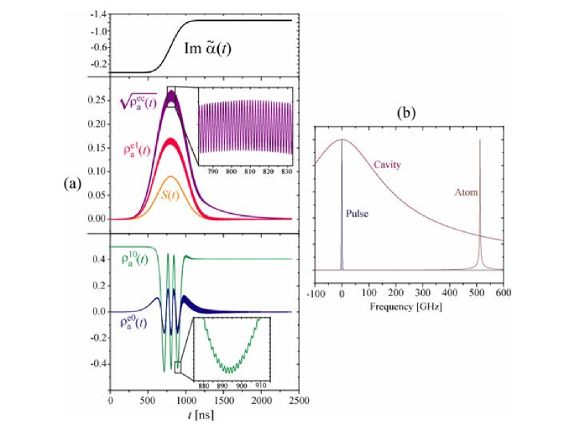
Figure 9: (a) Results from a typical simulation of the optical Bloch equations, using parameters $\alpha=100$, $g\sqrt{\kappa/\gamma}=20$ MHz, $\gamma=280$ MHz, and $\tau=300$ ns, typical of the ³¹P:Si system. The real parts of the off-diagonal elements of the density matrix are shown. (b) The spectra of the input pulse, cavity response, and ³¹P lineshape corresponding to this simulation.

A typical solution of these optical Bloch equations is shown in figure 9, using parameters typical of the ³¹P:Si system, as will be discussed in section 5. All simulations assume $F_{\rm\textsc{\scriptsize in}}(t)$ takes a Gaussian shape with root-mean-square time-pulse-width $\sigma_{{\rm\textsc{\scriptsize p}}}$. These simulations are performed using a standard adaptive Runge-Kutta solver. It is seen that ${\rm Im}\{\tilde{\alpha}(t)\}$ rises during the pulse and reaches an asymptotic value in accordance with the features predicted from both the perturbative analysis of section 4.3 and equation (35akbtbwcb). The off-diagonal elements $\varrho^{10}(t)$ and $\varrho^{{\rm e}0}(t)$ oscillate during the pulse due to the effective interaction with the light.

We may analyze the dynamics of $\varrho^{10}(t)$ and $\varrho^{{\rm e}0}(t)$ under a similar set of approximations under which we approximately solved the first three of the optical Bloch equations. We find

$${\varrho^{10}(t)}\rightarrow{\varrho^{10}(0)}\exp\biggl{(}-g^{2}\int_{0}^{\infty}\frac{\alpha^{*}\tilde{\alpha}(t)|S(t^{\prime})|^{2}}{\Gamma-i\Omega}dt^{\prime}\biggr{)}.$$ (35akbtbwcdcecfcg)

During the pulse, the qubit’s off-diagonal element $\varrho^{10}(t)$ shows a large oscillation with instantaneous frequency of approximately $g^{2}|\alpha S(t)|^{2}/\Omega$, proportional to the optical power inside the cavity. The reduction of the magnitude of this term is due to both the divergence of $\tilde{\alpha}(t)$ from $\alpha$, which is compensated for by returning the factor of $\bigl{\langle}\alpha\!\bigm{|}\!\tilde{\alpha}(t)\bigr{\rangle}$ to $\rho_{{\rm a}}^{10}(t)$, and dephasing due to the loss during the dispersive interaction. It is this effect that must be minimized for a high-fidelity gate.

The total magnitude of the damping to the desired coherence is calculated as

$$D(t)=e^{|\alpha-\tilde{\alpha}(t)|^{2}/2}\left|\frac{\varrho^{10}(t)}{\varrho^{10}(0)}\right|.$$ (35akbtbwcdcecfch)

The final fidelity of our qubit, assuming appropriate single-qubit phase corrections have been applied, may be written

$$F=1-2\bigl{|}\rho_{{\rm a}}^{10}(0)\bigr{|}^{2}\biggl{(}1-\lim_{t\rightarrow\infty}D(t)\biggr{)}.$$ (35akbtbwcdcecfci)

For the calculations presented here, we assume this interaction is being used for entanglement distribution, in which case we use $\rho_{{\rm a}}^{10}(0)=1/2$.

4.4.3 Approximate Optimization.

Figure 10: A sketch showing how the performance behaves as a function of $\Phi$ and the product of the pulse length and the decay rate, $\sigma_{{\rm\textsc{\scriptsize p}}}\Gamma$. In the hatched region, the pulse length is insufficient to achieve the desired distinguishability. Above that region, the fidelity improves somewhat with longer pulses and substantially with higher $\Phi$.

We now have enough approximations to estimate the optimum values of $\alpha$, $\Omega$, and the pulse width in order to obtain a desired distinguishability $d=\alpha\theta$ with a maximum fidelity. The roughness of our approximation is evident in the loose definition of $g^{2}|\bar{S}|^{2}$, which we suppose proportional to our estimate for the integral over $g^{2}|S(t)|^{2}$, $\Gamma\Phi$, divided by a measure of the length of the pulse, its pulse width $\sigma_{{\rm\textsc{\scriptsize p}}}$. We also assume, quite appropriately, that $\theta$ and $L$ are much less than one. For convenience, we use the unitless variable $y=\Omega/\Gamma$, the pulse detuning normalized by the width of the atomic line, which we assume is positive and much larger than 1. We also define

$$d_{{\rm m}}^{2}=\frac{\Phi^{2}\Gamma^{2}}{8g^{2}|\bar{S}|^{2}}\propto\Gamma\sigma_{{\rm\textsc{\scriptsize p}}}\Phi.$$ (35akbtbwcdcecfcj)

We may then summarize our approximations as

$$d \approx\frac{|\alpha|\Phi y}{1+y^{2}+|\alpha|^{2}\Phi^{2}/4d_{{\rm m}}^{2}},$$ (35akbtbwcdcecfck)

$$\log D \sim-\Phi|\alpha|^{2}\frac{1}{y^{2}}.$$ (35akbtbwcdcecfcl)

Our goal is to maximize $D$ while holding $d$ constant.

First, we note that the equation for $d$ may be rewritten as

$$\frac{d_{{\rm m}}}{d}=1+\frac{1+(y-x)^{2}}{2yx},$$ (35akbtbwcdcecfcm)

where $x=|\alpha|\Phi/2d_{{\rm m}}$. This equation shows clearly that no matter how large $\alpha\propto x$ is made, $d$ is always upper-bounded by $d_{{\rm m}}$. To reach a desired distinguishability, both $\Phi$ and the pulse width $\sigma_{{\rm\textsc{\scriptsize p}}}$ should be sufficiently large to assure $d_{{\rm m}}\geq d$.

For high fidelity, we must have $d_{{\rm m}}\gg d$ and work in an unsaturated regime. The optimum working condition is to work in the limit where $y\rightarrow\infty$ and $\alpha\rightarrow\infty$, keeping constant the ratio

$$2d_{{\rm m}}\frac{x}{y}=\frac{|\alpha|\Phi\Gamma}{\Omega}\approx d\biggl{(}1+\frac{d^{2}}{4d_{{\rm m}}^{2}}\biggr{)},$$ (35akbtbwcdcecfcn)

under which condition

$$D\sim\exp\biggl{[}-\frac{d^{2}}{\Phi}\biggl{(}1+\frac{d^{2}}{2d_{{\rm m}}^{2}}\biggr{)}\biggr{]}.$$ (35akbtbwcdcecfco)

These approximate results are sketched qualitatively in figure 10. Quantitatively, the critical values of the pulse width and $\Phi$ to achieve a useful fidelity should be calculated numerically, the results of which are shown in the next section.

5 Calculation of the Dispersive Light-Matter Interaction: Results

Besides an estimate for the fidelity, the discussion in the previous section provides a means of visualizing the output of numerical simulations. The ratio $x/y$ is proportional to $\alpha/\omega_{0}$ for systems with a small Purcell effect (either because the mode volume of the cavity is high or because $\omega_{0}\gg\gamma$). To make this a unitless number, we multiply by the normalizing frequency of the simulation. This timescale is the rate at which the atom couples to the cavity, $g$, but we note that in the equations of motion this parameter always appears as a product with the ratio $\sqrt{\kappa/\gamma}$, which indicates how well the cavity is overcoupled. We therefore combine these parameters into $g^{\prime}=g\sqrt{\kappa/\gamma}$; this single parameter $g^{\prime}$ encapsulates all the information about the atom’s oscillator strength and the cavity geometry. Using this normalization, the parameter $\alpha g^{\prime}/\omega_{0}$, indicates the degree to which the interaction is saturated, and therefore we call it the saturation parameter. We will plot observed distinguishabilities $d={\rm Im}\ \tilde{\alpha}$ and fidelities as a function of this saturation parameter.

We expect from the analysis above that the distinguishability will rise and reach a peak as a function of the saturation parameter. The peak value is $d_{{\rm m}}$ and occurs at $\alpha/\omega_{0}\approx 2d_{{\rm m}}/\Phi\Gamma.$ Therefore as the pulse length increases, the maximum increases and moves to higher values of $\alpha/\omega_{0}$. If the maximum reached is much larger than the desired distinguishability $d$, then the highest available fidelity is observed; lengthening the pulse duration only helps a small amount under this condition. Long pulse lengths do not appreciably slow down the proposal for entanglement distribution unless they approach the classical communication time between stations, which is about 50 $\mu$s for 10 km.

The behavior of $d$ and $F$ as a function of the saturation behavior should be approximately independent of the value of the product $\alpha\omega_{0}$, at least for small values of $\alpha/\omega_{0}$. The product $\alpha\omega_{0}$ becomes important at high values of the saturation parameter due to the Purcell effect.

In this section, we will see such plots for three important systems. We begin with the phosphorous donor impurity in a silicon microcavity, which has an intermediate value of $\Phi$. We will see improved performance in the high-$\Phi$ system of the flourine donor impurity in a ZnSe microcavity. We also consider a typical trapped ion in a macroscopic cavity, which may operate in the vicinity of $\Phi\sim 1$.

5.1 ³¹P:Si

The ³¹P donor impurity in silicon has become a favored system for several quantum information hardware proposals. An early, promising proposal for a quantum computer manipulated its electron and nuclear spins using electrostatic gates [25]. Since then, careful measurements of the electron spin decoherence time have been made [26]. These results indicate that isotopically purified silicon at low temperatures shows extremely long electron-spin coherence times approaching 60 ms.

The spin-1/2 ³¹P nucleus is a principal advantage of this impurity for a quantum repeater. In a quantum repeater system, very long coherence times are needed, as entanglement must be stored for at least the classical communication time over the long distances for which such systems are intended (1000–10000 km), and possibly much longer depending on the efficiency of the entanglement purification and entanglement swapping protocols. A long-distance repeater system will benefit from a many-second coherent quantum memory, and probably some form of quantum error correction. In semiconductors, only nuclei have shown coherence times this long [27]. A critical architecture component is therefore the existence of a nuclear spin to which coherence may be stored for long periods of time. While proposals for storing electron spin coherence in polarized nuclear ensembles have been considered, the degree of nuclear polarization required for both suppression of nuclear spin diffusion and high-fidelity nuclear memory do not appear to be practical. If a single nucleus such as ³¹P in Si is used, electron-nuclear transfer may be accomplished by electron-nuclear double-resonance techniques, as in the recent demonstration with nitrogen-vacancy centers in diamond [28]. Such transfer techniques were first considered in the electron-nuclear system of ³¹P:Si [18], and have been a strong candidate since some of the earliest proposals for experimental quantum information devices [29].

Recently, the optical characteristics of this important system have gathered much attention. The donor ground state features two Zeeman sublevels, providing the two lower levels of the desired $\Lambda$ system, and the state $\left|{\rm e}\right\rangle$ is provided by the lowest bound-exciton state. It was recently demonstrated that the optical bound-exciton transitions are extremely sharp [30], sharp enough to reveal the hyperfine splitting from the ³¹P nucleus [31]. Such sharp lines allow the measurement [32] of single nuclear spins and possibly optical electron-nuclear state transfer, a very rare possibility in semiconductors. Unfortunately, this system suffers from silicon’s poor optical efficiency. The radiative lifetime of the phonon-assisted bound-exciton to donor-ground-state transition is about 2 ms [33]. The more likely decay channel is Auger recombination, which occurs with lifetime 300 ns. This reduces the value of $\Phi$ for this system by a factor of $10^{4}$. Fortunately, however, microfabrication in silicon is an extremely mature technology. The existence of high-quality source material with small optical absorption and the wealth of techniques for etching silicon have led to very good lithographically fabricated photonic crystal microcavities, with $Q$-values of $10^{6}$ and mode-volumes on the order of $(\lambda/n)^{3}$ [34]. For this system, the Purcell effect makes the system optically active and therefore a strong candidate for a cqed quantum repeater. We estimate a coupling timescale of $g^{\prime}/2\pi=20{\rm~{}MHz}$. A $Q$ of $10^{6}$ leads to $\gamma/2\pi=280{\rm~{}MHz}$. The figure of merit $\Phi$ is then $11$.

Figure 11 shows the distinguishability $d$ and fidelity $F$ as a function of the saturation parameter $\alpha/\omega_{0}$ for this system. For low $\alpha/\omega_{0}$, the Purcell effect is not important and the dynamics depend little on the product $\alpha\omega_{0}$. The distinguishability and fidelity are improved at higher values of $\alpha$ and correspondingly smaller values of $\omega_{0}$.

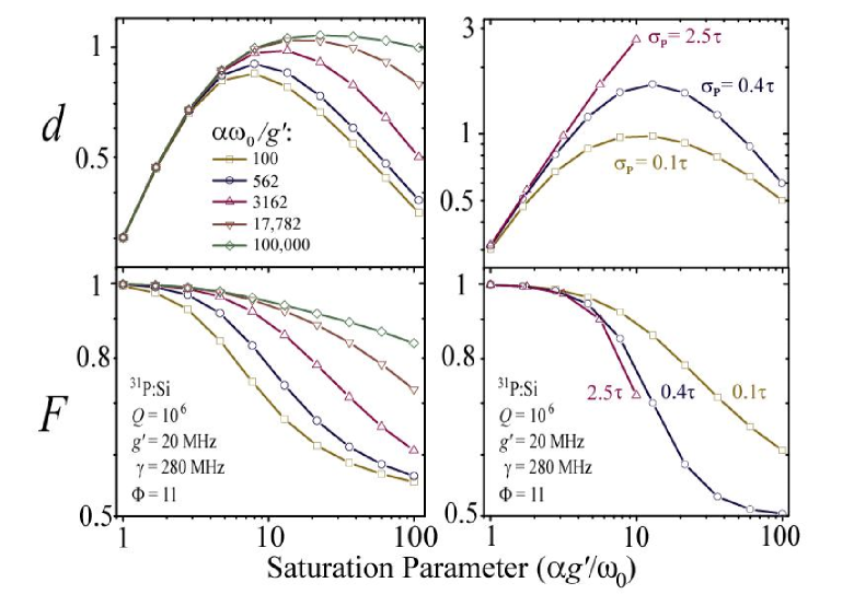
Figure 11: The top plots show the distinguishability as a function of the saturation parameter for ³¹P:Si. In each curve, $\alpha$ and $\omega_{0}$ are both varied while maintaining a constant value of $\alpha\omega_{0}$. The bottom plots show the fidelity of the interaction for the same parameters. The plots on the left are for $\sigma_{{\rm\textsc{\scriptsize p}}}=0.1\tau=30$ ns with varying values of $\alpha\omega_{0}$ shown. The plots on the right all use $\alpha\omega_{0}=3162g^{\prime}$ but with varying pulse lengths listed in terms of the Auger lifetime $\tau=300$ ns.

The pulse duration of $\sigma_{{\rm\textsc{\scriptsize p}}}=0.1\tau$ used in the left plots of figure 11 is insufficient to allow distinguishabilities greater than 1. To increase the maximum distinguishability, the pulse must be lengthened at same or higher values of $\alpha$. The right plots of figure 11 show how these curves change as the pulse length is increased, each keeping the product $\alpha\omega_{0}$ constant at 3162$g_{0}$. Note that the longest pulse considered in this simulation is still less than 1 $\mu$s.

For silicon, when the parameters describing the interaction are sufficiently strong to allow $d\sim 1.6$, Auger-limited fidelities greater than 95% are possible. This is sufficient fidelity for entanglement distribution, but is likely insufficient for efficient purification and entanglement swapping with the measurement-free C-$Z$ gate. For local operations, either higher-$Q$ cavities (which have been argued to be theoretically feasible [34]) or another implementation for local quantum logic would assist in efficient purification.

5.2 ¹⁹F:ZnSe

The flourine donor in ZnSe is a very promising system. Preliminary measurements [35] indicate that the radiative lifetime of the 440 nm bound-exciton to donor-ground-state transition is about 500 ps. Except for the wavelength, this system is therefore optically similar to charged quantum dots based on iii-v semiconductors. However, the ¹⁹F:ZnSe system shows some distinct advantages over iii-v systems. Bound exciton transitions are much more homogeneous in comparison to quantum dots. In comparison to bound excitons in GaAs, the higher binding energy and smaller Bohr radius of the ZnSe system suggests that it is more robust, easing the isolation of a single impurity in a fabricated microstructure. Most importantly, however, the decoherence of electrons in GaAs quantum dots or impurities is severely limited by nuclear spin diffusion, as every Ga and As nucleus has non-zero nuclear spin. In contrast, the only non-zero nuclear spins in ZnSe are the ⁶⁷Zn nucleus, which comprises only 4.1% of isotopically natural Zn, and ⁷⁷Se, which comprises only 7.6% of isotopically natural Se. The ¹⁹F impurity is convenient because ¹⁹F is 100% abundant and spin-1/2, like the ³¹P nucleus. The ¹⁹F:ZnSe system is therefore very similar in its nuclear environment to ³¹P:Si.

Perhaps the largest unknown about ZnSe is whether high-$Q$ microcavities may be fabricated from this material. Single impurities have been isolated in this material using wet-etching techniques [36], a promising start toward single impurities in ZnSe photonic crystal cavities. Cavities made from distributed Bragg reflectors and microposts are also a possibility. We believe it is realistic to expect microcavities with small mode volume $V\sim(\lambda/n)^{3}$ and moderate $Q$ values of at least $10^{3}$.

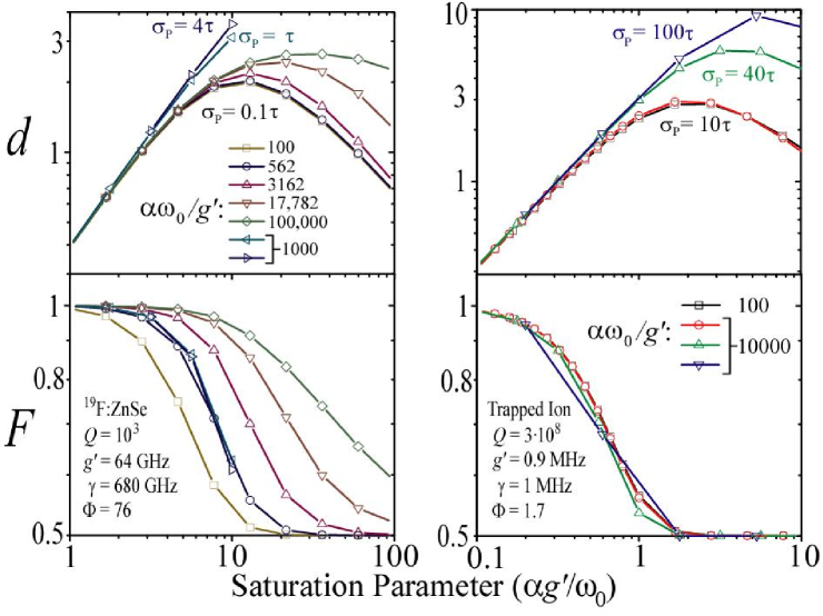
Figure 12: On the left are simulation results for ¹⁹F:ZnSe, and on the right are simulation results for a trapped ion, both plotted as in figure 11.

Using these parameters, simulations of this system yield distinguishabilities and fidelities as shown in figure 12. For pulses lasting several nanoseconds and $\alpha\sim 100$, fidelities above 99% are possible. This system is therefore a good candidate for both entanglement distribution and the measurement-free deterministic C-$Z$ gate. If the $Q$ can be made higher than $10^{3}$, the fidelity will only improve.

5.3 Trapped Ions

Among the longest lived coherences observed in the laboratory are the hyperfine states of trapped atoms or ions. Further, a large number of experiments have demonstrated the feasibility of quantum logic between multiple ions in a trap, and recent progress has been made toward scaling such experiments up to many qubits. For these reasons, trapped ions are promising candidates for quantum repeaters.

Unfortunately, it is very challenging to use a small-mode-volume cavity with an ion trap. Therefore, the Purcell factor will inevitably be limited. For typical parameters, consider the trapped ⁴⁰Ca ion/cavity systems reported in [37, 38, 39]. The atomic levels employed in these studies are not exactly the desired $\Lambda$ system, but we use values of $g$ and $\gamma$ from [39] as plausible parameters if such a system were employed. Although the cavity $Q$ is quite high ($\sim 3\times 10^{8}$), the large mode volume leads to the estimate $\Phi\sim 1.7$. As a result, the fidelity of the system is quite low. Simulation results are shown in figure 12. In this low-Purcell-factor regime the results are nearly independent of $\alpha\omega_{0}$, and the distinguishability depends strongly on the pulse-length. However, for the desired regime of $d\sim 1.6$, the fidelity is nearly unchanged after $\sigma_{{\rm\textsc{\scriptsize p}}}>10\tau$, indicating that further elongation of the pulses will allow only a marginal improvement. For the ion system, then, internal losses will be as important as external losses in determining the final entanglement fidelity.

6 Discussion & Conclusion

Most of the components of this proposal for a high-speed repeater are extremely practical with current technology. The light source is a filtered, power-stabilized laser with pulses that may be generated with normal modulation techniques. The detectors are not critical, and do not require abnormally large efficiency or low dark-count rates. The required fiber stabilization between repeater stations is available with current experimental techniques.

The only “exotic” element is the effective Hamiltonian of equation (4). However, our calculations show that this effective Hamiltonian is available in realistic emitter/cavity systems as long as the cooperativity parameter $\Phi$ is large. Such a system is well realized by semiconductor microcavity systems in the intermediate coupling regime. The ¹⁹F:ZnSe system and similar quantum dot systems in photonic crystal microcavities with reasonable $Q$-values show particular promise; here sufficiently large phase shifts are available to allow strongly-entangling distinguishabilities with interaction fidelities near 99%, resulting in strictly fiber-loss-limited initial entanglement fidelities. Even the optically dim ³¹P:Si system is reasonable with a sufficiently high-$Q$ microcavity. Trapped ion or trapped atom systems may be limited by large cavity mode volumes; in such systems the fidelity of the dispersive atom-cavity interaction may only be of order 80%. Even this system can in principle be well-utilized if sufficiently fast and accurate techniques for entanglement purification are employed.

Although dispersive interactions seem to be strong enough for entanglement distribution, a remaining question is whether these systems can be employed for scalable, fault-tolerant quantum computation using techniques such as those described in [15]. This will ultimately depend on the error-correcting protocols employed. The problem of a quantum repeater system is somewhat less stringent since errors of several percent during purification and swapping are tolerable [12]. The use of measurement-free C-$Z$ gates with the finite fidelities calculated in the present study should allow some rate of purification and swapping to allow scalable long-distance communication. Our calculation of communication rates approaching 100 Hz for repeater stations every 10 km of a total distance of 1280 km was provided as an example; higher speeds or longer station-to-station distances are possible. Future theoretical development of this proposal will involve optimizing the details of the entanglement purification and swapping protocol.

Appendix A Loss Analysis of Deterministic C-Sign Gate

A wide range of errors are possible for the measurement free C-$Z$ gate described in section 3.4: the displacements may be imperfect in magnitude and phase, the single-qubit rotations may be imperfect, and of course each interaction of the optical bus with a cavity introduces some external loss and some internal loss. For internal loss, the fidelity calculations presented in Sections 4 and 5 apply, but in real optical systems external losses are always an issue, so we focus on those errors here.

The first operation in the gate is the dispersive interaction described in section 3. To this we must add the displacement of the coherent bus. Although some loss may be associated with the displacement, the result of this loss is not very different from the result if the loss occurred during the the cavity-light interaction either preceding or following the displacement, and therefore we associate loss with the cavity-light interaction as described in section 3.2. For example, after the first interaction a loss characterized by transmission $T_{1}$ is assumed to occur; the first displacement in the C-$Z$ gate is then altered to $\sqrt{T_{1}}\alpha_{1}(i-1)$, where $\alpha_{1}$ would ideally have the same phase and magnitude as $\alpha_{0}$, but in practice may be slightly different. Since this displacement is purely unitary, we may keep track of its operation on the ket resulting from equation (12):

$$D\bigl{[}(i-1)\sqrt{T_{1}}\alpha_{1}\bigr{]}\biggl{|}\sqrt{T_{1}}\beta_{1}(Z_{1})\biggr{\rangle}=e^{iT_{1}{\rm Im}\{\beta_{1}^{*}(i-1)\alpha_{1}\}}\biggl{|}\sqrt{T_{1}}[\beta_{1}(Z_{1})+(i-1)\alpha_{1}]\biggr{\rangle}.$$ (35akbtbwcdcecfcp)

If the bus state now interacts with a second qubit, the resulting state is

$$\eqalign{\Tr_{{\rm\textsc{l}}}{U_{2}D\bigl{[}(i-1)\sqrt{T_{1}}\alpha_{1}\bigr{]}U_{1}\bigl{|}\alpha_{0}\bigr{\rangle}\rho\bigl{\langle}\alpha_{0}\bigr{|}U_{1}^{\dagger}D^{\dagger}\bigl{[}(i-1)\sqrt{T_{1}}\alpha_{1}\bigr{]}U_{2}^{\dagger}}=\\ e^{iT_{1}{\rm Im}\{\beta_{1}^{*}\alpha_{1}(i-1)\}}\biggl{|}\sqrt{T_{1}T_{2}}\beta_{2}(Z_{1},Z_{2})\biggr{\rangle}Q_{2}(Q_{1}(\rho))\biggl{\langle}\sqrt{T_{1}T_{2}}\beta_{2}(Z_{1},Z_{2})\biggr{|}e^{-iT_{1}{\rm Im}\{\beta_{1}^{*}\alpha_{1}(i-1)\}},}$$ (35akbtbwcdcecfcq)

where we have traced over lost photons. The superoperator $Q_{2}(\rho)$ is substantially more complicated than $Q_{1}(\rho)$. In general, at the $n$th step in the gate, we may write $Q_{n}(\rho)$ in the $Z$-basis as

$$\eqalign{Q_{n}(\rho)=\sum_{jk,mn}\left|jk\right\rangle\!\!\left\langle jk\right|\rho\left|mn\right\rangle\!\!\left\langle mn\right|\times\\ \exp\biggl{[}-(1-T_{n})T_{n-1}T_{n-2}\cdots\biggl{(}\frac{|\beta_{n}(j,k)-\beta_{n}(m,n)|^{2}}{2}+i{\rm Im}\{\beta_{n}^{*}(j,k)\beta_{n}^{\phantom{*}}(m,n)\}\biggr{)}\biggr{]},}$$ (35akbtbwcdcecfcr)

where $j$ and $k$ enumerate the eigenstates of $Z_{1}$ and $Z_{2}$, as do $m$ and $n$. It is worthwhile to point out here that $Q_{n}$ will in general contain state-dependent phase shifts, and that these will contribute to the C-$Z$ gate as well as the Berry phases which accrue during displacements.

This type of analysis may be carried through to the end of the gate. The full sequence of operations is

$$U_{4}D\bigl{[}(1-i)\sqrt{T_{1}T_{2}T_{3}}\alpha_{3}\bigr{]}U_{3}D\bigl{[}(-1-i)\sqrt{T_{1}T_{2}}\alpha_{2}\bigr{]}U_{2}D\bigl{[}(-1+i)\sqrt{T_{1}}\alpha_{1}\bigr{]}U_{1},$$ (35akbtbwcdcecfcs)

where $U_{3}$ and $U_{4}$ correspond to couplings back to qubits 1 and 2, respectively, but may have different transmissions $T_{j}$ and angles $\theta_{j}$ due to imperfect coupling in the optical circuit. As a result of this sequence, the total state-dependent Berry phase that develops is given by

$$\eqalign{\phi_{{\rm\textsc{b}}}(Z_{1},Z_{2})=\\ {\rm Im}\{(i-1)T_{1}\beta_{1}^{*}(Z_{1})\alpha_{1}-(i+1)T_{1}T_{2}\beta_{2}^{*}(Z_{1},Z_{2})\alpha_{2}-(i-1)T_{1}T_{2}T_{3}\beta_{3}^{*}(Z_{1},Z_{2})\alpha_{3}\}.}$$ (35akbtbwcdcecfct)

At the end of the gate, the coherent bus photons are lost; i.e we may use $T_{4}=0$ with equation (35akbtbwcdcecfcr) to find the final superoperator $Q_{4}(\rho)$ after losing the bus state.

With this formalism, several errors in the C-$Z$ gate may be analyzed in general. Here we suppose that the displacements are accomplished perfectly (every $\alpha_{j}$ is the same in magnitude and phase), and every interaction with every cavity is exactly the same, hence studying only errors due to optical loss. We call this the semi-ideal case. Also, we work to second order in $\theta$, as this is the lowest non-vanishing order after correction of single-qubit phase shifts.

In this semi-ideal case the coherent state amplitudes witnessed by the bus state during the gate are

$$\beta_{1}(Z_{1},Z_{2}) =|\alpha|^{2}\biggl{[}1+i\frac{\theta}{2}Z_{1}-\frac{\theta^{2}}{8}\biggr{]},$$ (0a)

$$\beta_{2}(Z_{1},Z_{2}) =|\alpha|^{2}\biggl{[}i+\frac{\theta}{2}(iZ_{1}-Z_{2})-\frac{\theta^{2}}{8}(1+i+2Z_{1}Z_{2})\biggr{]},$$ (0b)

$$\beta_{3}(Z_{1},Z_{2}) =|\alpha|^{2}\biggl{[}-1-\frac{\theta}{2}Z_{2}-\frac{\theta^{2}}{8}[1+(1+i)(1+2Z_{1}Z_{2})]\biggr{]},$$ (0c)

$$\beta_{4}(Z_{1},Z_{2}) =|\alpha|^{2}\biggl{[}-i-\frac{\theta^{2}}{4}(1+i)(1+Z_{1}Z_{2})\biggr{]},$$ (0d)

and the Berry phase simplifies to

$$\phi_{{\rm\textsc{b}}}=|\eta\alpha|^{2}\biggl{\{}\bigl{[}1+T+T^{2}\bigr{]}+\frac{\theta}{2}\bigl{[}(1+T)(Z_{1}+TZ_{2})\bigr{]}+\frac{\theta^{2}}{8}\bigl{[}3T^{2}-1+2T(1+2T)Z_{1}Z_{2}\bigr{]}\biggr{\}}.$$ (1)

We see that this may be immediately decomposed into a global phase (due to constant terms), single-qubit rotations (single $Z$ terms), and a nonlinear term going as $Z_{1}Z_{2}$. This last term is part of the nonlinearity leading to the C-$Z$ gate.

However, extra phases occur due to the superoperators $Q_{n}$, which resulted from “which-path” information carried away by lost photons or the optical bus. To second order in $\theta$ in the semi-ideal case,

$$\eqalign{Q_{4}(Q_{3}(Q_{2}(Q_{1}(\rho))))=\\ e^{i|\alpha|^{2}[(1-T)(Z_{1}+TZ_{2})\theta/2+T^{2}(1-2T)Z_{1}Z_{2}\theta^{2}/4]}D(\rho)e^{-i|\alpha|^{2}[(1-T)(Z_{1}+TZ_{2})\theta/2+T^{2}(1-2T)Z_{1}Z_{2}\theta^{2}/4]},}$$ (2)

where we have seperated out pure rotations and C-$Z$ terms from a distortion operator $D(\rho)$, which may in general be generated from equation (35akbtbwcdcecfcr) in the computational basis as $D(\rho)=\sum_{jk,mn}\mathcal{D}_{jk,mn}\left|jk\right\rangle\!\!\left\langle jk\right|\rho\left|mn\right\rangle\!\!\left\langle mn\right|$. The matrix $\mathcal{D}$ is Hermitian with unity diagonal. In the semi-ideal case, to lowest order in $\theta$, the off-diagonal elements are

$$\mathcal{D}_{++,+-}=\mathcal{D}_{--,-+} =e^{-[T(1-T^{2})-iT(1-T)]|\alpha\theta|^{2}/2-|\alpha\theta^{2}|^{2}/4},$$ (0a)

$$\mathcal{D}_{++,-+}=\mathcal{D}_{--,+-} =e^{-[\phantom{T}(1-T^{2})+iT(1-T)]|\alpha\theta|^{2}/2-|\alpha\theta^{2}|^{2}/4},$$ (0b)

$$\mathcal{D}_{++,--}=\mathcal{D}_{+-,-+} =e^{-(1-T^{2})(1+T)|\alpha\theta|^{2}/2}.$$ (0c)

Terms of order $\theta^{4}$ are present to show that there is distortion even if there is no loss in the system ($T=1$).

For the operation of the C-$Z$ gate, we presume the single-qubit rotations from the semi-ideal case $\exp{i(1+T^{2})(Z_{1}+\eta^{2}Z_{2})}|\alpha|^{2}\theta/2$ are removed. Imperfect correction of these phase shifts may be an important form of error, as these shifts are of order $|\alpha|^{2}\theta,$ which will be much larger than $\pi$. Neglecting these shifts and the global phase shift, the resulting unitary operation from this gate is the very simple

$$U_{{\rm C-}Z}=\exp\biggl{(}iT(1+T)\frac{|\alpha\theta|^{2}}{4}Z_{1}Z_{2}\biggr{)}.$$ (1)

To make this a C-$Z$ gate, we must choose $T(1+T)|\alpha\theta|^{2}=\pi,$ and add single-qubit rotations $\exp[-i(\pi/4)(Z_{1}+Z_{2})]$.

For a general case, the distortions due to errors are more computationally convenient to express as a sum of Kraus operators. Let $\lambda_{m}$ be the eigenvalues of the matrix $\mathcal{D}/4$, and define $A=H_{2}T$, where $H_{2}$ is the usual 2-qubit Hadamard transformation and the columns of $T$ are the orthonormal eigenvectors of $\mathcal{D}$. Then the distortion superoperator may be written

$$D(\rho)=\sum_{m}D_{m}\rho D_{m}^{\dagger}$$ (2)

where

$$D_{m}=\sqrt{\lambda_{m}}\bigl{(}A_{++,m}+A_{+-,m}Z_{2}+A_{-+,m}Z_{1}+A_{--,m}Z_{1}Z_{2}\bigr{)}.$$ (3)

For example, we used such a description for the $Q_{1}$ superoperator, with only two noise components, $D_{+}=\sqrt{\lambda_{+}}\exp{iZ_{1}\xi_{1}/2}$ and $D_{-}=\sqrt{\lambda_{-}}Z_{1}\exp{iZ_{1}\xi_{1}/2}$. The eigenvalues $\lambda_{m}$ are in general calculated numerically. The only operator with an identity element is $D_{0}$, corresponding to the largest eigenvalue $\lambda_{0}$. Therefore the deviation from unity of $\lambda_{0}$ characterizes the fidelity of the gate. For $\theta^{2}\ll\sqrt{T}$, which is the appropriate regime for the systems considered in this paper, the largest eigenvalue $\lambda_{0}$ is approximately $(1+\exp(-\pi\sqrt{T}/4))^{2}/4$. Numerical results for several values of $\theta$ are shown in figure 7.

The distortion operators $D_{m}$ commute with the desired C-$Z$ gate. To generate a controlled-not, or C-$X$ gate, we must simply rotate the target qubit, qubit 2, with $\exp(-i\pi Y/4)$. Therefore the final noisy operation describing a C-$X$ gate in the presence of optical loss is

$$U_{{\rm C-}X}^{\phantom{{\dagger}}}\sum_{m}\tilde{D}_{m}^{\phantom{{\dagger}}}\rho\tilde{D}_{m}^{\dagger}U_{{\rm C-}X}^{\dagger},$$ (4)

where

$$\tilde{D}_{m}=\sqrt{\lambda_{m}}\bigl{(}A_{++,m}+A_{+-,m}X_{2}+A_{-+,m}Z_{1}+A_{--,m}Z_{1}X_{2}\bigr{)}.$$ (5)

These operators fully describe the error model which may be used in an analysis of entanglement purification schemes or error-correction techniques.

Appendix B Phase-Shift Calculation with Finite-Order Cumulant Expansion

In this Appendix we detail an approach for calculating the state-dependent phase shift due to a single atom-cavity interaction in the dispersive limit. Here we calculate the phase shift and internal loss assuming the atom begins in state $\left|1\right\rangle$.

We perform a finite-order cumulant expansion, in which we write

$$\chi(\eta,t)=\chi(\eta,0)\exp[\Psi(\epsilon,\eta,t)].$$ (6)

The function $\Psi(\epsilon,\eta,t)$ vanishes at $\epsilon=0$ and $t=0$; for $\epsilon>0$ it may be expanded in a Taylor series

$$\Psi(\epsilon,\eta,t)=\epsilon\Psi_{1}(\eta,t)+\frac{\epsilon^{2}}{2}\Psi_{2}(\eta,t)+\ldots$$ (7)

This may be compared to the Taylor series for $\chi(\eta,t)$:

$$\chi(\eta,t)=\chi_{0}(\eta,t)\biggl{[}1+\epsilon\Psi_{1}+\frac{\epsilon^{2}}{2}(\Psi_{2}+\Psi_{1}^{2})+\ldots\biggr{]},$$ (8)

the latter of which we actually calculate to finite order.

To find each order, we solve the Liouville-von Neumann equation for the atom-cavity coupling. The iterative solution is

$$\tilde{\rho}(t)=\sum_{k=0}^{\infty}\epsilon^{k}\rho_{k}(t),$$ (9)

where $\rho_{0}=\rho(t=0)$. We again work with Laplace transforms, with which we find

$$\rho_{k}(s)=-\frac{i}{s}\oint\frac{dq_{1}}{2\pi i}\oint\frac{dq_{2}}{2\pi i}\frac{[\tilde{\mathcal{H}}_{{\rm int}}(q_{1}),\rho_{k-1}(q_{2})]}{s-q_{1}-q_{2}}+\frac{1}{s}\mathcal{L}[\rho_{k-1}(s)],$$ (10)

where in the inverse transform we must close the $s$ contour to the right of all $q_{1},q_{2}$. Using equation (35akc), $\rho_{k}(s)$ may be found from

$$\rho_{k}(s)={ig\sqrt{\kappa}}\sum_{m}\oint\frac{dq}{2\pi i}\biggl{[}\frac{F_{m}(q)}{q+z}a_{m}\sigma^{+}+\frac{F_{m}^{*}(q)}{q+z^{*}}a_{m}^{\dagger}\sigma^{-},\frac{\rho_{k-1}(s-q)}{s}\biggr{]}+\frac{1}{s}\mathcal{L}[\rho_{k-1}(s)],$$ (11)

where for compact notation we define $z=i\omega_{0}+\gamma/2$ and $F_{0}(q)=-1/\sqrt{\kappa}$. The first few terms are

$$\rho_{0}(s)= \frac{1}{s}\left|\alpha\right\rangle\!\!\left\langle\alpha\right|\otimes\sigma^{-}\sigma^{+}$$

$$\rho_{1}(s)= ig\sqrt{\kappa}\biggl{\{}\alpha\frac{F_{\rm\textsc{\scriptsize in}}(s)}{s(s+z)}\left|\alpha\right\rangle\!\!\left\langle\alpha\right|\sigma^{+}-{\rm h.c.}\biggr{\}}$$

$$\rho_{2}(s)= -g^{2}\kappa\sum_{m}\biggl{\{}A_{m}^{(1)}(s)\bigl{[}a_{m}^{\dagger}\sigma^{-},\alpha\left|\alpha\right\rangle\!\!\left\langle\alpha\right|\sigma^{+}\bigr{]}+{\rm h.c.}\biggr{\}}-\frac{1}{2s\tau}\rho_{1}(s)$$

$$\rho_{3}(s)= +\frac{g^{2}\kappa}{2\tau}\sum_{m}\biggl{\{}A_{m}^{(2)}(s)\bigl{[}a_{m}^{\dagger}\sigma^{-},\alpha\left|\alpha\right\rangle\!\!\left\langle\alpha\right|\sigma^{+}\bigr{]}+{\rm h.c.}\biggr{\}}-\frac{1}{(2s\tau)^{2}}\rho_{1}(s)$$

$$-2\frac{g^{2}\gamma}{s\tau}{\rm Re}\bigl{\{}A_{\rm\textsc{\scriptsize in}}(s)\bigr{\}}|\alpha|^{2}\left|\alpha\right\rangle\!\!\left\langle\alpha\right|\sigma^{z}$$

$$-ig^{3}\kappa^{3/2}\sum_{m}\oint\frac{dq}{2\pi i}\frac{1}{s(q+z)}\biggl{\{}F_{m}(q)A_{m}(s-q)\left|\alpha\right\rangle\!\!\left\langle\alpha\right|+$$

$$\phantom{ig^{3}\gamma^{3/2}\sum_{m}\oint\frac{dq}{2\pi i}}{F_{m}(q)}\bigl{[}A_{\rm\textsc{\scriptsize in}}(s-q)+A_{\rm\textsc{\scriptsize in}}^{*}(s-q)\bigr{]}\alpha^{*}\left|\alpha\right\rangle\!\!\left\langle\alpha\right|a_{m}$$

$$\phantom{ig^{3}\gamma^{3/2}\sum_{m}\oint\frac{dq}{2\pi i}}+{F_{\rm\textsc{\scriptsize in}}(q)}\bigl{[}A_{m}(s-q)a_{m}^{\dagger}\alpha\left|\alpha\right\rangle\!\!\left\langle\alpha\right|+A_{m}^{*}(s-q)\left|\alpha\right\rangle\!\!\left\langle\alpha\right|\alpha^{*}a_{m}\bigr{]}\biggr{\}}\alpha\sigma^{+},$$

where

$$A_{m}^{(j)}(s)=\oint\frac{dq}{2\pi i}\frac{F_{m}^{*}(q)F_{\rm\textsc{\scriptsize in}}(s-q)}{s(s-q)^{j}(q+z^{*})(s-q+z)}.$$ (12)

The two lowest non-vanishing terms of the Laplace transform of $\Psi(\epsilon,\eta,t)$ are then found as

$$\frac{\epsilon^{2}}{2}\Psi_{2}(\eta,s) =\chi_{0}^{-1}(\eta)\Tr\{\tilde{D}_{\rm\textsc{\scriptsize out}}(\eta)\rho_{2}(s)\}=+g^{2}\kappa A^{(1)}_{\rm\textsc{\scriptsize in}}(s)\eta^{*}\alpha-{\rm c.c.}$$ (0a)

$$\frac{\epsilon^{3}}{6}\Psi_{3}(\eta,s) =\chi_{0}^{-1}(\eta)\Tr\{\tilde{D}_{\rm\textsc{\scriptsize out}}(\eta)\rho_{3}(s)\}=-\frac{g^{2}\kappa}{2\tau}A^{(2)}_{\rm\textsc{\scriptsize in}}(s)\eta^{*}\alpha-{\rm c.c.},$$ (0b)

where “c.c.” refers to complex conjugate. Again, we are interested only in the asymptotic $t\rightarrow\infty$ limit. All poles of $A(s)$ with negative real part may be ignored. Poles with imaginary part also damp out since the pulse has finite duration. Only the $s=0$ pole is important. We write $q=i\omega$ and note that the denominator $(s-i\omega)^{-1}$ may be written $i/\omega+\pi\delta(\omega)$, resulting in

$$A_{\rm\textsc{\scriptsize in}}^{(1)}(t)\rightarrow-i\ {\rm p.v.}\!\int\frac{d\omega}{2\pi}\frac{|F(-i\omega)|^{2}}{\omega|z-i\omega|^{2}}-\frac{1}{2}\frac{|F(0)|^{2}}{|z|^{2}}.$$ (1)

From these expressions we obtain the estimates discussed in section 4.3.

References

References

- [1] For a review, see Raimond J M, Brune M and Haroche S 2001 Rev. Mod. Phys. 73, 565, section viii. A similar experiment is Turchette Q A, Hood C J, Lange W, Mabuchi M and Kimble H J 1995 Phys. Rev. Lett. 75, 4710.
- [2] P. Horak, B. G. Klappauf, A. Haase, R. Folman, J. Schmiedmayer, P. Domokos, and E. A. Hinds. Phys. Rev. A, 67:43806, 2003.
- [3] R. Long, T Steinmets, P. Hommelhoff, W. Hänsel, T. W. Hänsch, and J. Reichel. Phil. Trans. R. Soc. Lond. A, 361:1375, 2003.
- [4] J. J. Hope and J. D. Close. Phys. Rev. Lett., 93:180402, 2004.
- [5] P. van Loock, T. D. Ladd, K. Sanaka, F. Yamaguchi nad K. Nemoto, W. J. Munro, and Y. Yamamoto. Phys. Rev. Lett., 96:240501, 2006.
- [6] J. I. Cirac, P. Zoller, H. J. Kimble, and H. Mabuchi. Phys. Rev. Lett., 78:3221, 1997.
- [7] S. J. van Enk, J. I. Cirac, and P. Zoller. Phys. Rev. Lett., 78:4293, 1998.
- [8] L. M. Duan, M. D. Lukin, J. I. Cirac, and P. Zoller. Nature, 414:413, 2001.
- [9] L. Childress, J. M. Taylor, A. S. Sørensen, and M. D. Lukin. Phys. Rev. A, 72:52330, 2005.
- [10] E. Waks and J. Vuckovic. Phys. Rev. Lett., 96:153601, 2006.
- [11] W. Yao, R-B. Liu, and L. J. Sham. Phys. Rev. Lett., 95:030504, 2005.
- [12] W. Dür, H. J. Briegel, J. I. Cirac, and P. Zoller. Phys. Rev. A, 59:169, 1999.
- [13] C. W. Chou, H. de Riedmatten, D. Felinto, S. V. Polyakov, S. J. van Enk, and H. J. Kimble. Nature, 438:828, 2005.
- [14] L.-M. Duan and H. J. Kimble. Phys. Rev. Lett., 92:127902, 2004.
- [15] T. P. Spiller, K. Nemoto, S. L. Braunstein, W. J. Munro, P. van Loock, and G. J. Milburn. New J. Phys, 8:30, 2006.
- [16] D. Deutsch, A. Ekert, R. Jozsa, C. Macchiavello, S. Popescu, and A. Sanpera. Phys. Rev. Lett., 77:2818, 1996.
- [17] P. Chen, C. Piermarocchi, L. J. Sham, D. Gammon, and D. G. Steel. Phys. Rev. B, 69:75320, 2004.
- [18] G. Feher. Phys. Rev., 114:1219, 1959.
- [19] C. Langrock, E. Diamanti, R. V. Roussev, Y. Yamamoto, M. M. Fejer, and H. Takesue. Opt. Lett., 30:1725, 2005.
- [20] S. Tanzilli, W. Tittel, M. Halder, O. Alibart, P. Baldi, N. Gisin, and H. Zbinden. Nature, 437:116, 2005.
- [21] K. Nemoto and W. J. Munro. Phys. Rev. Lett., 93:250502, 2004.
- [22] W. J. Munro, K. Nemoto, and T. P. Spiller. New J. Phys., 7:137, 2005.
- [23] D. F. Walls and G. J. Milburn. Quantum Optics. Springer, 1994.
- [24] Y. Zu, R. K. Lee, and A. Yariv. Phys. Rev. A, 61:33807, 2000.
- [25] B. E. Kane. Nature, 393:133, 1998.
- [26] A. M. Tyryshkin, S. A. Lyon, A. V. Astashkin, and A. M. Raitsimring. Phys. Rev. B, 68:193207, 2003.
- [27] T. D. Ladd, D. Maryenko, Y. Yamamoto, E. Abe, and K. M. Itoh. Phys. Rev. B, 71:14401, 2005.
- [28] F. Jelezko, T. Gaebel, I. Popa, M. Domhan, A. Gruber, and J. Wrachtrup. Phys. Rev. Lett., 93:130501, 2004.
- [29] D. P. DiVincenzo. Science, 270:255, 1995.
- [30] D. Karaiskaj and M. L. W. Thewalt and T. Ruf and M. Cardona and H.-J. Pohl and G. G. Deviatych and P. G. Sennikov and H. Riemann. Phys. Rev. Lett., 86:6010, 2001.
- [31] M. L. W. Thewalt. private communication.
- [32] K-M. C. Fu, T. D. Ladd, C. Santori, and Y. Yamamoto. Phys. Rev. B, 69:125306, 2004.
- [33] W. Schmid. Phys. Status Solidi B, 84:529, 1977.
- [34] B.-S. Song, S. Noda, T. Asano, and Y. Akahane. Nature Materials, 4:207, 2005.
- [35] K. Sanaka. private communication.
- [36] S. Strauf, P. Michler, M. Klude, D. Hommel, G. Bacher, and A. Forchel. Phys. Rev. Lett., 89:177403, 2002.
- [37] G. R. Guthöhrlein, M. Keller, K. Hayasaka, W. Lange, and H. Walther. Nature, 414:49, 2001.
- [38] A. B. Mundt, A. Kreuter, C. Becher, D. Leibfried, J. Eschner, F. Schmidt-Kaler, and R. Blatt. Phys. Rev. Lett., 89:103001, 2002.
- [39] M. Keller, B. Lange, K. Hayasaka, W. Lange, and H. Walther. Eur. Phys. J. D, 32:161, 2005.