Key Words: Teleportation, Braid group, Temperley–Lieb algebra

PACS numbers: 03.65.Ud, 02.10.Kn, 03.67.Lx

1 Introduction

Quantum entanglements [1] play key roles in quantum information phenomena [2] and they are widely exploited in quantum algorithms [3, 4], quantum cryptography [5, 6] and quantum teleportation [7]. On the other hand, topological entanglements [8] represent topological configurations like links or knots which are closures of braids. There are natural similarities between quantum entanglements and topological entanglements. As a unitary braid has a power of detecting knots or links, it often can transform a separate quantum state into an entangled one. Hence a nontrivial unitary braid representation can be identified with a universal quantum gate [9, 10]. Recently, a series of papers have been published on the application of knot theory to quantum information, see [11, 12, 13] for universal quantum gates and unitary solutions of the Yang–Baxter equation [14, 15]; see [16, 17, 18] for quantum topology and quantum computation; see [19, 20] for quantum entanglements and topological entanglements.

Especially, Kauffman’s work on the teleportation topology [11, 21] motivates our tour of revisiting in a diagrammatic approach all tight teleportation and dense coding schemes in Werner’s paper [22]. Under the project of setting up a bridge between knot theory and quantum information, the joint paper with Kauffman and Werner [23] explores topological and algebraic structures underlying multipartite entanglements by recognizing the Werner state as a rational solution of the Yang–Baxter equation and the isotropic state as a braid representation, and constructing a representation of the Temperley–Lieb algebra in terms of maximally entangled states, while the present paper focuses on the problem of how to study the teleportation from the viewpoints of the braid group and Temperley–Lieb algebra [24].

The teleportation is a kind of quantum information protocol transporting a unknown quantum state. To describe it in a unified mathematical formalism, we have to integrate standard quantum mechanics with classical features since outcomes of quantum measurements are sent to Bob from Alice via classical channels and then Bob carries out a required unitary operation. The one approach has been proposed by Abramsky and Coecke in recent research. It applies the category theory to quantum information protocols and describes the quantum information flow by strongly compact closed categories, see [25, 26] for abstract physical traces; see [27, 28] for the quantum information flow; see [29, 30] for a categorical description of quantum protocols; see [31, 32, 33] for diagrammatic quantum mechanics and see [34] for quantum logic.

As Abramsky and Coecke suggest [35], we also expect a powerful mathematical framework to describe quantum information phenomena in a unified framework. We believe in the existence of beautiful mathematical structures underlying entanglement and teleportation such as the braid group and Temperley–Lieb algebra which are well known to the community of knot theory for a long time. They not only simplify complicated algebraic calculations in an intuitive manner but also catch essential points of quantum phenomena and exhibit them in a natural style.

A maximally entangled bipartite state is found to form a representation of the Temperley–Lieb algebra. In view of the diagrammatic representation for the Temperley–Lieb algebra, we are inspired to deal with quantum information protocols involving maximally entangled states in a diagrammatic approach. We think that diagrams catch essential points from the global view so that they can express complicated algebraic objects in a simpler way. We represent maximally entangled vectors by cups or caps because they are widely exploited in topics including the Temperley–Lieb algebra, braid representations, knot theory and statistics mechanics [8].

Section 2 revisits the quantum teleportation from the viewpoints of the braid group and virtual braid group [36, 37, 38, 39]. The transformation matrix between the Bell states and product bases is found to form a braid representation and this stimulates us to propose the braid teleportation configuration together with the teleportation swapping and explain it with the crossed measurement [40, 41, 42]. Also, the virtual mixed relation for defining the virtual braid group is found to be a formulation of the teleportation equation.

Section 3 devises diagrammatical rules for quantum information protocols involving maximally entangled states, projective measurements and local unitary transformations. Various properties of maximally entangled states are collected and these guide us to set up diagrammatical rules for assigning a definite diagram to a given algebraic expression. Three types of descriptions for the quantum teleportation phenomena: the transfer operator [43], quantum measurements [40, 41, 42] and characteristic equations [22], are respectively revisited in our diagrammatical approach.

Section 4 proposes the Temperley–Lieb algebra under local unitary transformations to be a suitable mathematical structure underlying the quantum teleportation phenomena. The connections between the diagrammatical representation for the Temperley–Lieb algebra and our diagrammatical approach are made as clear as possible. The teleportation configuration is recognized as a fundamental ingredient for defining the Brauer algebra [44], and it can be performed in terms of swap gates and Bell measurements.

Section 5 sketches two known diagrammatical approaches to the quantum information flow: Kauffman’s teleportation topology [11, 21] and the categorical theory mainly considered by Abramsky and Coecke, which are compared with our diagrammatical approach in order to stress conceptual differences in both physics and mathematics among them and propose our diagrammatical rules to present a natural diagrammatic language for the teleportation phenomena.

Section 6 is on concluding remarks and outlooks. Our next steps in this promising research are discussed in a brief way.

2 Teleportation, braid group and virtual braid group

Based on the teleportation equation in terms of the Bell matrix for the standard description of the quantum teleportation phenomena, we realize the braid configuration $(b^{-1}\otimes Id)(Id\otimes b)$ together with the teleportation swapping $(P\otimes Id)(Id\otimes P)$, and explain it via the concept of the crossed measurement [40, 41, 42]. We also study the teleportation in terms of a virtual braid representation.

2.1 Teleportation equation in terms of Bell matrix

In terms of product bases $|ij\rangle$, $i,j=0,1$, the four mutually orthogonal Bell states have the forms,

$$|\phi^{+}\rangle=\frac{1}{\sqrt{2}}(|00\rangle+|11\rangle),\qquad|\phi^{-}\rangle=\frac{1}{\sqrt{2}}(|00\rangle-|11\rangle),$$

$$|\psi^{+}\rangle=\frac{1}{\sqrt{2}}(|01\rangle+|10\rangle),\qquad|\psi^{-}\rangle=\frac{1}{\sqrt{2}}(|01\rangle-|10\rangle),$$ (1)

which are transformed to each other under local unitary transformations,

$$|\phi^{-}\rangle=(1\!\!1_{2}\otimes\sigma_{3})|\phi^{+}\rangle=(\sigma_{3}\otimes 1\!\!1_{2})|\phi^{+}\rangle,$$

$$|\psi^{+}\rangle=(1\!\!1_{2}\otimes\sigma_{1})|\phi^{+}\rangle=(\sigma_{1}\otimes 1\!\!1_{2})|\phi^{+}\rangle,$$

$$|\psi^{-}\rangle=(1\!\!1_{2}\otimes-i\sigma_{2})|\phi^{+}\rangle=(i\sigma_{2}\otimes 1\!\!1_{2})|\phi^{+}\rangle,$$ (2)

where $1\!\!1_{2}$ denotes a $2\times 2$ unit matrix, so $1\!\!1_{d}$ for a $d\times d$ unit matrix, and the Pauli matrices $\sigma_{1}$, $\sigma_{2}$ and $\sigma_{3}$ have the conventional formalisms.

The teleportation is a quantum information protocol of sending a message $|\psi\rangle_{C}$ from Charlie to Bob under the help of Alice . Alice, who shares a maximally entangled state $|\phi^{+}\rangle_{AB}$ with Bob, performs an entangling measurement on the composite system between Charlie and her and then informs results of her measurements to Bob, who will know what Charlie wants to pass onto him according to a protocol between Alice and him. Note the following calculation, also see [43],

$$|\psi\rangle_{C}|\phi^{+}\rangle_{AB}\equiv\frac{1}{\sqrt{2}}(a|0\rangle+b|1\rangle)_{C}(|00\rangle+|11\rangle)_{AB}$$

$$= \frac{1}{2}(|\phi^{+}\rangle_{CA}|\psi\rangle_{B}+|\phi^{-}\rangle_{CA}\sigma_{3}|\psi\rangle_{B}+|\psi^{+}\rangle_{CA}\sigma_{1}|\psi\rangle_{B}+|\psi^{-}\rangle_{CA}(-i\sigma_{2})|\psi\rangle_{B})$$

which is called the teleportation equation and tells how to teleport a qubit $|\psi\rangle_{C}$ from Charlie to Bob. When Alice detects the Bell state $|\phi^{+}\rangle_{CA}$ and informs Bob about that through a classical channel, Bob will know that he has a quantum state $|\psi\rangle_{B}$. Similarly, when Alice gets the Bell states $|\phi^{-}\rangle_{CA}$ or $|\psi^{+}\rangle_{CA}$ or $|\psi^{-}\rangle_{CA}$, Bob will apply the local unitary transformations $\sigma_{3}$ or $\sigma_{1}$ or $i\sigma_{2}$ on the quantum state that he has in order to obtain $|\psi\rangle_{B}$.

We introduce the Bell matrix [11, 12, 10] and denote it by $B=(B_{ij,\,lm})$, $i,j,l,m=0,1$. The Bell matrix and its inverse or transpose are given by

$$B=\frac{1}{\sqrt{2}}\left(\begin{array}[]{cccc}1&0&0&1\\ 0&1&-1&0\\ 0&1&1&0\\ -1&0&0&1\\ \end{array}\right),\qquad B^{-1}=B^{T}=\frac{1}{\sqrt{2}}\left(\begin{array}[]{cccc}1&0&0&-1\\ 0&1&1&0\\ 0&-1&1&0\\ 1&0&0&1\\ \end{array}\right).$$ (4)

It has an exponential formalism given by

$$B=e^{i\frac{\pi}{4}(\sigma_{1}\otimes\sigma_{2})}=\cos{\frac{\pi}{4}}+i\sin\frac{\pi}{4}(\sigma_{1}\otimes\sigma_{2})$$ (5)

with the following interesting properties:

$$B^{2}=i\sigma_{1}\otimes\sigma_{2},\qquad B^{4}=-1\!\!1_{4},\qquad B^{8}=1\!\!1_{4},\qquad B=\frac{1}{\sqrt{2}}(1\!\!1_{4}+B^{2}).$$ (6)

In terms of the Bell matrix and product bases, the Bell states can be generated in the formalism,

$$|\phi^{+}\rangle=B|11\rangle,\qquad|\phi^{-}\rangle=B|00\rangle,$$

$$|\psi^{+}\rangle=B|01\rangle,\qquad|\psi^{-}\rangle=-B|10\rangle$$ (7)

where the Bell operator acts on product bases in the way,

$$B|ij\rangle=\sum_{k,l=0}^{1}|kl\rangle B_{kl,ij}=\sum_{k,l=0}^{1}|kl\rangle B^{T}_{ij,kl},$$ (8)

and hence the teleportation equation (2.1) can be rewritten into a new formalism,

$$(1\!\!1_{2}\otimes B)(|\psi\rangle\otimes|11\rangle)_{CAB}\equiv(B\otimes 1\!\!1_{2})({\vec{v}}^{T}\otimes\frac{1}{2}{\vec{\sigma}}_{11}|\psi\rangle)_{CAB},$$ (9)

where the vectors $\vec{\sigma}_{11}$ and $\vec{v}$ are convenient notations, their transposes given by

$$\vec{\sigma}_{11}^{T}\equiv(\sigma_{3},\sigma_{1},i\sigma_{2},1\!\!1_{2}),\qquad{\vec{v}}^{T}\equiv(|00\rangle,|01\rangle,|10\rangle,|11\rangle)$$ (10)

and the calculation of ${\vec{v}}^{T}\otimes{\vec{\sigma}}_{11}$ follows a rule:

$${\vec{v}}^{T}\otimes{\vec{\sigma}}_{11}|\psi\rangle\equiv|00\rangle\otimes\sigma_{3}|\psi\rangle+|01\rangle\otimes\sigma_{1}|\psi\rangle+|10\rangle\otimes i\sigma_{2}|\psi\rangle+|11\rangle\otimes|\psi\rangle.$$ (11)

The remaining three teleportation equations are derived in the same way by applying local unitary transformations among the Bell states (2.1) to the teleportation equation (9). As a maximally entangled state shared by Alice and Bob is $|\phi^{-}\rangle_{AB}$, the teleportation equation has the form

$$|\psi\rangle_{C}|\phi^{-}\rangle_{AB}=(1\!\!1_{2}\otimes B)(|\psi\rangle\otimes|00\rangle)_{CAB}$$ (12)

$$= |\psi\rangle_{C}\otimes(1\!\!1_{2}\otimes\sigma_{3})|\phi^{+}\rangle_{AB}=(B\otimes 1\!\!1_{2})({\vec{v}}^{T}\otimes\frac{1}{2}\sigma_{3}{\vec{\sigma}}_{11}|\psi\rangle)_{CAB}$$

where the local unitary transformation $1\!\!1_{2}\otimes 1\!\!1_{2}\otimes\sigma_{3}$ commutes with $B\otimes 1\!\!1_{2}$. Similarly, the other two teleportation equations are obtained in the following,

$$(B^{-1}\otimes 1\!\!1_{2})(1\!\!1_{2}\otimes B)(|\psi\rangle\otimes|01\rangle)_{CAB}=({\vec{v}}^{T}\otimes\frac{1}{2}\sigma_{1}{\vec{\sigma}}_{11}|\psi\rangle)_{CAB},$$

$$(B^{-1}\otimes 1\!\!1_{2})(1\!\!1_{2}\otimes B)(|\psi\rangle\otimes-|10\rangle)_{CAB}=({\vec{v}}^{T}\otimes-\frac{1}{2}i\sigma_{2}{\vec{\sigma}}_{11}|\psi\rangle)_{CAB}.$$ (13)

It is obvious that the matrix configuration $(B^{-1}\otimes 1\!\!1_{2})(1\!\!1_{2}\otimes B)$ plays a key role in the above teleportation equations in terms of the Bell matrix.

2.2 Braid teleportation configuration $(b^{-1}\otimes Id)(Id\otimes b)$

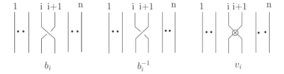
Figure 1: Braid generators $b_{i}$, $b_{i}^{-1}$ and virtual braid generator $v_{i}$.

We sketch the definitions for the braid group and virtual braid group and verify the Bell matrix $B$ to form a braid representation and virtual braid representation. We propose the braid teleportation configuration $(b^{-1}\otimes Id)(Id\otimes b)$ with the teleportation swapping as its special example, and explain it in terms of the crossed measurement [40].

A braid representation $b$-matrix is a $d\times d$ matrix acting on $V\otimes V$ where $V$ is a $d$-dimensional complex vector space. The symbol $b_{i}$ denotes a braid $b$ acting on the tensor product $V_{i}\otimes V_{i+1}$, see Figure 1 where $b_{i}$ is described by a under crossing and its inverse $b_{i}^{-1}$ is represented by an over crossing. The classical braid group $B_{n}$ is generated by braids $b_{1},b_{2}$, $\cdots,b_{n-1}$ satisfying the braid relation, see Figure 2,

$$b_{i}b_{j} = b_{j}b_{i},\qquad j\neq i\pm 1,$$

$$b_{i}b_{i+1}b_{i} = b_{i+1}b_{i}b_{i+1},\qquad i=1,\cdots,n-2.$$ (14)

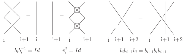
Figure 2: Identity and the braid relation.

The virtual braid group $VB_{n}$ [36, 37, 38, 39] is an extension of the classical braid group $B_{n}$ by the symmetric group $S_{n}$. It has both braids $b_{i}$ and virtual crossings $v_{i}$ which are defined by the virtual crossing relation,

$$v_{i}^{2} = 1\!\!1,\qquad v_{i}v_{i+1}v_{i}=v_{i+1}v_{i}v_{i+1},\qquad i=1,\cdots,n-2,$$

$$v_{i}v_{j} = v_{j}v_{i},\qquad j\neq i\pm 1,$$ (15)

a presentation of the symmetric group $S_{n}$, and the virtual mixed relation:

$$b_{i}v_{j} = v_{j}b_{i},\qquad j\neq i\pm 1,$$

$$b_{i+1}v_{i}v_{i+1} = v_{i}v_{i+1}b_{i},\qquad i=1,\cdots,n-2.$$ (16)

See Figure 1-2. A virtual crossing $v_{i}$ is represented by two crossing arcs with a small circle placed around a crossing point. In virtual crossings, we do not distinguish between under and over crossings but which are described respectively in the classical knot theory. The identity $Id$ is represented by parallel vertical straight lines without any crossings.

We verify the Bell matrix to satisfy the braid relation (2.2). On its right handside of (2.2), after a little algebra we have

$$(1\!\!1_{2}\otimes B)(B\otimes 1\!\!1_{2})(1\!\!1_{2}\otimes B)=\frac{1}{\sqrt{2}}(1\!\!1_{2}\otimes B^{2}+B^{2}\otimes 1\!\!1_{2})$$ (17)

and on its left handside we can derive the same result. We now prove the Bell matrix to satisfy the virtual mixed relation (2.2) as the permutation matrix $P$ is chosen as a virtual crossing,

$$P=\left(\begin{array}[]{cccc}1&0&0&0\\ 0&0&1&0\\ 0&1&0&0\\ 0&0&0&1\end{array}\right),\qquad P|ij\rangle=|ji\rangle,\qquad i,j=0,1.$$ (18)

On the left handside of (2.2), we derive

$$(1\!\!1_{2}\otimes B)(P\otimes 1\!\!1_{2})(1\!\!1_{2}\otimes P)(|i\rangle\otimes|j\rangle\otimes|k\rangle)=(1\!\!1_{2}\otimes B)(|k\rangle\otimes|ij\rangle)$$ (19)

which can be also obtained via the right handside of (2.2).

Figure 3: Teleportation swapping with permutation $P$ as virtual crossing.

In view of the fact that the braid configuration $(B^{-1}\otimes 1\!\!1_{2})(1\!\!1_{2}\otimes B)$ is the most important element in the above teleportation equation (9), we propose the concept of the braid teleportation configuration $(b^{-1}\otimes Id)(Id\otimes b)$. Since a braid is a kind of generalization of permutation, we call $(P\otimes Id)(Id\otimes P)$ or $(Id\otimes P)(P\otimes Id)$ as the teleportation swapping, which satisfy

$$|k\rangle\otimes|ij\rangle=(P\otimes Id)(Id\otimes P)(|ij\rangle\otimes|k\rangle),$$

$$|ij\rangle\otimes|k\rangle=(Id\otimes P)(P\otimes Id)(|k\rangle\otimes|ij\rangle).$$ (20)

See Figure 3, the permutation $P$ represented by a virtual crossing with a small circle at the crossing point. In the crossed measurement [40], a braid or crossing acts as a device of measurement which is non-local in both space and time. In Figure 4, the two lines of a crossing $b$ represent two observable operations: the first relating the measurement at the space-time point $(x_{1},t_{1})$ to that at the other point $(x_{2},t_{2})$ and the second one relating the measurement at $(x_{1},t_{2})$ to that at $(x_{2},t_{1})$. The crossed measurement $(Id\otimes b)$ plays a role of sending a qubit from Charlie to Alice with a possible local unitary transformation. Similarly, the crossed measurement $(b^{-1}\otimes Id)$ transfers a qubit from Alice to Bob with a possible local unitary transformation.

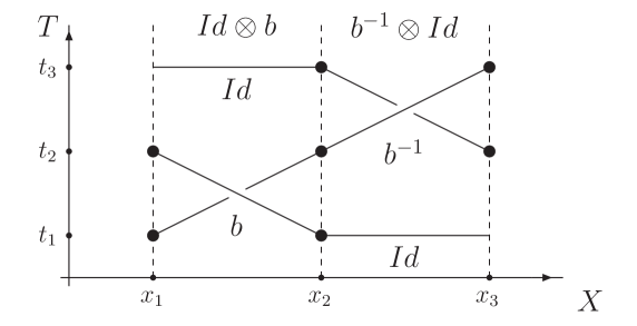
Figure 4: Braid teleportation configuration and crossed measurement.

2.3 Teleportation and virtual braid group

We describe the teleportation in the framework of the virtual braid group: The braid relation (2.2) builds a connection between topological entanglements and quantum entanglements, while the virtual mixed relation (2.2) is a sort of reformulation of the teleportation equation (2.1). A nontrivial unitary braid detecting knots or links can be identified with a universal quantum gate transforming a separate state into an entangled one, see [11, 12, 13]. In the following, we make a connection clear between the virtual mixed relation (2.2) and the teleportation equation (2.1).

In terms of the Bell matrix and teleportation swapping, the left handside of the teleportation equation (2.1) has a form,

$$|\psi\rangle_{C}\otimes|\phi^{+}\rangle_{AB}=(1\!\!1_{2}\otimes B)(P\otimes 1\!\!1_{2})(1\!\!1_{2}\otimes P)(|11\rangle_{CA}\otimes|\psi\rangle_{B}),$$ (21)

while its right handside, $RHS$ leads to a formalism,

$$RHS=(1\!\!1_{2}\otimes P-1\!\!1_{2}\otimes\sigma_{2}\otimes\sigma_{2})(B\otimes 1\!\!1_{2})(|11\rangle_{CA}\otimes|\psi\rangle_{B})$$ (22)

where the permutation matrix $P$ (18) is given by

$$P=\frac{1}{2}(1\!\!1_{4}+\sigma_{1}\otimes\sigma_{1}+\sigma_{2}\otimes\sigma_{2}+\sigma_{3}\otimes\sigma_{3}),$$ (23)

and local unitary transformations (2.1) among the Bell states are used. Hence the teleportation equation (2.1) has a new formulation given by

$$|\psi\rangle_{C}\otimes|\phi^{+}\rangle_{AB}=(1\!\!1_{2}\otimes P-1\!\!1_{2}\otimes\sigma_{2}\otimes\sigma_{2})(|\phi^{+}\rangle_{CA}\otimes|\psi\rangle_{B}).$$ (24)

This equation (24) is an equivalent realization of the teleportation swapping on the state $|\phi^{+}\rangle_{CA}\otimes|\psi\rangle_{B}$:

$$(1\!\!1_{2}\otimes P-1\!\!1_{2}\otimes\sigma_{2}\otimes\sigma_{2})(|\phi^{+}\rangle_{CA}\otimes|\psi\rangle_{B})=(P\otimes 1\!\!1_{2})(1\!\!1_{2}\otimes P)(|\phi^{+}\rangle_{CA}\otimes|\psi\rangle_{B}),$$ (25)

and it can be regarded as a formulation of the virtual mixed relation (2.2) on the state $|11\rangle_{CA}\otimes|\psi\rangle_{B}$,

$$(1\!\!1_{2}\otimes B)(P\otimes 1\!\!1_{2})(1\!\!1_{2}\otimes P)(|11\rangle_{CA}\otimes|\psi\rangle_{B})$$

$$=(P\otimes 1\!\!1_{2})(1\!\!1_{2}\otimes P)(B\otimes 1\!\!1_{2})(|11\rangle_{CA}\otimes|\psi\rangle_{B}).$$ (26)

Similarly, the teleportation equations for the Bell state $|\phi^{-}\rangle_{AB}$, $|\psi^{\pm}\rangle_{AB}$ are respectively obtained to be

$$|\psi\rangle_{C}\otimes|\phi^{-}\rangle_{AB} = (1\!\!1_{2}\otimes P-1\!\!1_{2}\otimes\sigma_{1}\otimes\sigma_{1})(|\phi^{-}\rangle_{CA}\otimes|\psi\rangle_{B}),$$

$$|\psi\rangle_{C}\otimes|\psi^{+}\rangle_{AB} = (1\!\!1_{2}\otimes P-1\!\!1_{2}\otimes\sigma_{3}\otimes\sigma_{3})(|\psi^{+}\rangle_{CA}\otimes|\psi\rangle_{B}),$$

$$|\psi\rangle_{C}\otimes|\psi^{-}\rangle_{AB} = (1\!\!1_{2}\otimes P-1\!\!1_{8})(|\psi^{-}\rangle_{CA}\otimes|\psi\rangle_{B}),$$ (27)

in which local unitary transformations of $(1\!\!1_{2}\otimes P-1\!\!1_{2}\otimes\sigma_{2}\otimes\sigma_{2})$ have been exploited. All of them can be identified with realizations of the virtual mixed relation (2.2) or the teleportation swapping.

3 Diagrammatical representations for teleportation

We devise diagrammatical rules for describing maximally entangled states in a diagrammatical approach and apply them to three typical descriptions of the quantum teleportation phenomena: the transfer operator, quantum measurements and characteristic equations.

3.1 Notations for maximally entangled states

Maximally entangled states have various good algebraic properties and they play important roles in the quantum teleportation phenomena. Here we fix our notations for maximally entangled states. The vectors $|e_{i}\rangle$ form a set of complete and orthogonal bases for a $d$-dimension Hilbert space $\cal H$, and the covectors $\langle e_{i}|$ are chosen for its dual Hilbert space ${\cal H}^{\ast}$, i.e., they satisfy

$$\sum_{i=0}^{d-1}|e_{i}\rangle\langle e_{i}|=1\!\!1_{d},\qquad\langle e_{j}|e_{i}\rangle=\delta_{ij},\qquad i,j=0,1,\cdots d-1,$$ (28)

where $\delta_{ij}$ is the Kronecker symbol.

A maximally entangled bipartite vector $|\Omega\rangle$ and its dual vector $\langle\Omega|$ have the forms

$$|\Omega\rangle=\frac{1}{\sqrt{d}}\sum_{i=0}^{d-1}|e_{i}\otimes e_{i}\rangle,\qquad\langle\Omega|=\frac{1}{\sqrt{d}}\sum_{i=0}^{d-1}\langle e_{i}\otimes e_{i}|.$$ (29)

The local action of a bounded linear operator $M$ in the Hilbert space $\cal H$ on $|\Omega\rangle$ satisfies

$$(M\otimes 1\!\!1_{d})|\Omega\rangle=(1\!\!1_{d}\otimes M^{T})|\Omega\rangle,\qquad M_{ij}\equiv\langle e_{i}|M|e_{j}\rangle,\,\,\,M^{T}_{ij}=M_{ji},$$ (30)

and so it is permitted to move the local action of the operator $M$ from the Hilbert space to the other Hilbert space as $M$ acts on $|\Omega\rangle$. A trace of two operators $M^{\dagger}$ and $M^{\prime}$ can be represented by an inner product of two quantum vectors $|\psi\rangle$ and $|\psi^{\prime}\rangle$,

$$tr(M^{\dagger}M^{\prime})=d\,\langle\psi|\psi^{\prime}\rangle,\qquad|\psi\rangle\equiv(M\otimes 1\!\!1_{d})|\Omega\rangle,\,\,\,|\psi^{\prime}\rangle\equiv(M^{\prime}\otimes 1\!\!1_{d})|\Omega\rangle,$$ (31)

while an inner product with the action of an operator product $N_{1}\otimes N_{2}$ is also a form of trace,

$$\langle\psi|N_{1}\otimes N_{2}|\psi^{\prime}\rangle=\frac{1}{d}tr(M^{\dagger}N_{1}M^{\prime}N_{2}^{T}).$$ (32)

The transfer operator $T_{BC}$ sending a quantum state from Charlie to Bob,

$$T_{BC}\equiv\sum_{i=0}^{d-1}|e_{i}\rangle_{B}\,\,{}_{C}\langle e_{i}|,\qquad T_{BC}|\psi\rangle_{C}=|\psi\rangle_{B},$$ (33)

is recognized to be an inner product between maximally entangled vectors $|\Phi(U)\rangle_{CA}$ and $|\Phi(V^{T})\rangle_{AB}$ defined by local unitary actions of $U$ and $V^{T}$ on $|\Omega\rangle$, i.e.,

$${}_{CA}\langle\Phi(U)|\Phi(V^{T})\rangle_{AB}\equiv{}_{CA}\langle\Omega|(U^{\dagger}\otimes 1\!\!1_{d})(V^{T}\otimes 1\!\!1_{d})|\Omega\rangle_{AB}$$

$$={}_{CAB}\langle\Omega\otimes 1\!\!1_{d}|(U^{\dagger}\otimes 1\!\!1_{d}\otimes 1\!\!1_{d})(1\!\!1_{d}\otimes V^{T}\otimes 1\!\!1_{d})|1\!\!1_{d}\otimes\Omega\rangle_{CAB}$$

$$=\frac{1}{d}(VU^{\dagger})_{B}\,\,T_{BC}$$ (34)

which has a special case of $U=V$ given by

$$\frac{1}{d}T_{BC}={}_{CA}\langle\Phi(U)|\Phi(U^{T})\rangle_{AB}={}_{CA}\langle\Omega|\Omega\rangle_{AB}.$$ (35)

A maximally entangled vector $|\Omega_{n}\rangle$ is a local unitary transformation of $|\Omega\rangle$, i.e., $|\Omega_{n}\rangle=(U_{n}\otimes 1\!\!1_{d})|\Omega\rangle$, and the set of local unitary operators $U_{n}$ satisfies the orthogonal relation $tr(U_{n}^{\dagger}U_{m})=d\,\delta_{nm}$, which leads to the fundamental properties of $|\Omega_{n}\rangle$,

$$\langle\Omega_{n}|\Omega_{m}\rangle=\delta_{nm},\qquad\sum_{n=1}^{d^{2}}|\Omega_{n}\rangle\langle\Omega_{n}|=1\!\!1_{d},\qquad n,m=1,\cdots,d^{2}.$$ (36)

We introduce the symbol $\omega_{n}$ to denote a maximally entangled state $|\Omega_{n}\rangle\langle\Omega_{n}|$ and especially use the symbol $\omega$ to represent $|\Omega\rangle\langle\Omega|$, i.e.,

$$\omega\equiv|\Omega\rangle\langle\Omega|,\qquad\omega_{n}\equiv|\Omega_{n}\rangle\langle\Omega_{n}|,\qquad U_{1}=1\!\!1_{d},\,\,\,\,\,\sum_{n=1}^{d^{2}}\omega_{n}=1\!\!1_{d},$$ (37)

where $\omega_{n}$ is a projector since $\omega_{n}^{2}=\omega_{n}$, $n=1,\,\cdots,\,d^{2}$, representing a set of observables over an output parameter space.

3.2 Diagrammatical rules for maximally entangled states

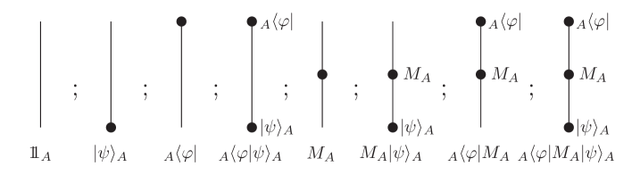
Figure 5: Straight lines without or with points.

Our diagrammatical rules assign a definite diagram to a given algebraic expression: Every diagrammatic element is mapped to an algebraic term. They consist of three parts: the first for our convention; the second for straight lines and oblique lines; the third for cups and caps.

Rule 1. Read an algebraic expression such as an inner product from the left to the right and draw a diagram from the top to the bottom.

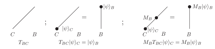
Figure 6: Oblique line for transfer operator.

Rule 2. See Figure 5. A straight line of type $A$ denotes an identity for the system $A$, which is a linear combination of projectors. Straight lines of type $A$ with top or bottom boundary solid points describe a vector $|\psi\rangle_{A}$, a covector ${}_{A}\langle\varphi|$, and an inner product ${}_{A}\langle\varphi|\psi\rangle_{A}$ for the system $A$, respectively. Straight lines of type $A$ with a middle solid point and top or bottom boundary solid points describe an operator $M_{A}$, a covector ${}_{A}\langle e_{i}|M_{A}$, a vector $M_{A}|\psi\rangle_{A}$ and an inner product ${}_{A}\langle\varphi|M_{A}|\psi\rangle_{A}$, respectively. See Figure 6: An oblique line connecting the system $C$ to the system $B$ describes the transfer operator $T_{BC}$ and its solid points have the same interpretations as those on a straight line of type $A$.

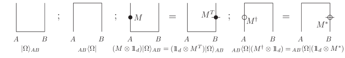
Figure 7: Cups and caps without or with points.

Rule 3. See Figure 7. A cup denotes a maximally entangled vector $|\Omega\rangle$ and a cap does for its dual $\langle\Omega|$. A cup with a middle solid point at its one branch describes the local action of an operator $M$ on $|\Omega\rangle$. This solid point flows to the other branch and becomes a solid point with a cross line representing $M^{T}$ due to (30). The same things happen for a cap except that a solid point is replaced by a small circle to distinguish the operator $M$ from its transposed and complex conjugation $M^{\dagger}=(M^{T})^{\ast}$.

A cup and a cap can generate several kinds of configurations. See Figure 8. As a cup is at the top and a cap is at the bottom for the same composite system, such a configuration is assigned to a projector $|\Omega\rangle\langle\Omega|$. As a cap is at the top and a cup is at the bottom for the same composite system, this configuration describes an inner product $\langle\Omega|\Omega\rangle=1$ by a closed circle. As a cup is at the bottom for the composite system ${\cal H}_{C}\otimes{\cal H}_{A}$ and a cap is at the top for the composite system ${\cal H}_{A}\otimes{\cal H}_{B}$, the diagram is equivalent to an oblique line representing the transfer operator $T_{BC}$ from Charlie to Bob.

Additionally, see Figure 8. As a cup has a local action of the operator $M$ and a cap has a local action of the operator $N^{\dagger}$, a resulted circle with a solid point for $M$ and a small circle for $N^{\dagger}$ represents a trace $\frac{1}{d}tr(MN^{\dagger})$. As conventions, we describe a trace of operators by a closed circle with solid points or small circles. We assign each cap or cup a normalization factor $\frac{1}{\sqrt{d}}$ and a circle a normalization factor $d$ according to the trace of $1\!\!1_{d}$.

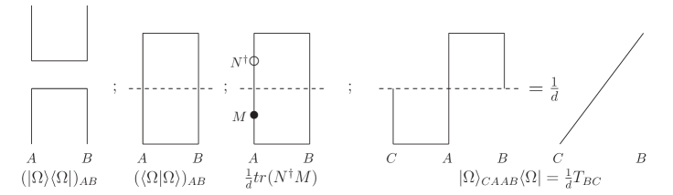
Figure 8: Three kinds of combinations of a cup and a cap.

3.3 Description of teleportation (I): the transfer operator

Besides its standard description [7] for the teleportation equation (2.1), the teleportation can be explained in terms of the transfer operator $T_{BC}$ (33) which sends a quantum state from Charlie to Bob in the way: $T_{BC}|\psi\rangle_{C}=|\psi\rangle_{B}$, also see [43]. In the following, we repeat the above algebraic calculation in (3.1) for the transfer operator $T_{BC}$ at the diagrammatic level and then discuss the so called acausality problem.

From the left to the right, the inner product ${}_{CA}\langle\Phi(U)|\Phi(V^{T})\rangle_{AB}$ consists of the cap $\langle\Omega|$, identity $1\!\!1_{d}$, local unitary operators $U$ and $V^{T}$, identity $1\!\!1_{d}$ and cup $|\Omega\rangle$ which are drawn from the top to the bottom, see Figure 9. Move the local operators $U^{\dagger}$ and $V^{T}$ along the line from their positions to the top boundary point of the system $B$ and obtain the local product $(VU^{\dagger})_{B}$ of unitary operators acting on a quantum state that Bob has. The normalization factor $\frac{1}{d}$ is from vanishing of a cup and a cap. Hence the quantum teleportation can be regarded as a flow of quantum information from Charlie to Bob.

But the operator product $\frac{1}{d}(VU^{\dagger})_{B}T_{BC}$ seems to argue that the quantum measurement with the unitary operator $U^{\dagger}$ plays a role before the state preparation with the unitary operator $V^{T}$. It is not true. Let us read Figure 9 in the way where the $T$-axis denotes a time arrow and the $X$-axis denotes a space distance. The quantum information flow starts from the state preparation, goes to the quantum measurement and come backs to the state preparation again and finally goes to the quantum measurement. As a result, it flows from the state preparation to the quantum measurement without violating the causality principle.

Note that we have to impose an additional rule on how to move operators in our diagrammatic approach: It is forbidden for an operator to cross over another operator. For example, we have the operator product $\frac{1}{d}(VU^{\dagger})_{B}$ instead of $\frac{1}{d}(U^{\dagger}V)_{B}$, see Figure 9. Obviously, the violation of this rule leads to the violation of the causality principle.

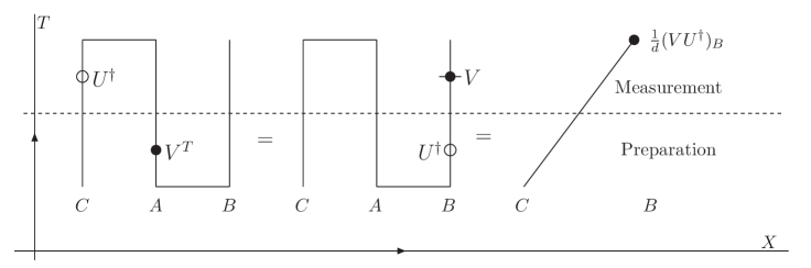
Figure 9: Transfer operator and acausality problem.

3.4 Description of teleportation (II): quantum measurements

Teleportation has an interpretation via quantum measurements [40, 41, 42, 45]. The difference from the standard description [7] of the teleportation is that the maximally entangled state $|\Omega\rangle_{AB}$ between Alice and Bob is created in the non-local measurement [40]. Here we simply represent the quantum measurement in terms of the projector $(|\Omega\rangle\langle\Omega|)_{AB}$.

Therefore, the teleportation is determined by two quantum measurements: the one denoted by $(|\Omega\rangle\langle\Omega|)_{AB}$ and the other denoted by $(|\Omega_{n}\rangle\langle\Omega_{n}|)_{CA}$. This leads to a new formulation of the teleportation equation,

$$(|\Omega_{n}\rangle\langle\Omega_{n}|\otimes 1\!\!1_{d})(|\psi\rangle\otimes|\Omega\rangle\langle\Omega|)=\frac{1}{d}(|\Omega_{n}\rangle\otimes 1\!\!1_{d})(1\!\!1_{d}\otimes(1\!\!1_{d}\otimes U_{n}^{\dagger}|\psi\rangle)\langle\Omega|),$$ (38)

where the lower indices $A,B,C$ are omitted for convenience.

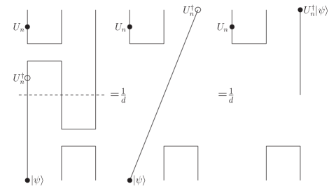
Figure 10: Teleportation based on quantum measurements.

Read the teleportation equation (38) from the left to the right and draw a diagram from the top to the bottom in view of our rules, i.e., Figure 10. There is a natural connection between two formalisms (2.1) and (38) of the teleportation equation. Choose all unitary matrices $U_{n}$ in the way so that they satisfy (36) and then make a summation of all independent teleportation equations like (38) to derive the version (2.1) of the teleportation equation in the $d$-dimension Hilbert space,

$$|\psi\rangle\otimes|\Omega\rangle=\frac{1}{d}\sum_{n=1}^{d^{2}}|\Omega_{n}\rangle\otimes U_{n}^{\dagger}|\psi\rangle.$$ (39)

In the case of $d=2$, the collection of unitary operators consists of the unit matrix $1\!\!1_{2}$ and Pauli matrices $\sigma_{1},\sigma_{2},\sigma_{3}$. The Bell measurements are denoted by projectors in terms of the Bell states $|\phi^{\pm}\rangle$ and $|\psi^{\pm}\rangle$, and they satisfy

$$1\!\!1_{2}=|\phi^{+}\rangle\langle\phi^{+}|+|\phi^{-}\rangle\langle\phi^{-}|+|\psi^{+}\rangle\langle\psi^{+}|+|\psi^{-}\rangle\langle\psi^{-}|.$$ (40)

We have the following teleportation equations, the same type as (38),

$$(|\phi^{-}\rangle\langle\phi^{-}|\otimes 1\!\!1_{2})(|\psi\rangle\otimes|\phi^{+}\rangle)=\frac{1}{2}(|\phi^{-}\rangle\otimes\sigma_{3}|\psi\rangle),$$

$$(|\psi^{+}\rangle\langle\psi^{+}|\otimes 1\!\!1_{2})(|\psi\rangle\otimes|\phi^{+}\rangle)=\frac{1}{2}(|\psi^{+}\rangle\otimes\sigma_{1}|\psi\rangle),$$

$$(|\psi^{-}\rangle\langle\psi^{-}|\otimes 1\!\!1_{2})(|\psi\rangle\otimes|\phi^{+}\rangle)=\frac{1}{2}(|\psi^{-}\rangle\otimes-i\sigma_{2}|\psi\rangle),$$

$$(|\phi^{+}\rangle\langle\phi^{+}|\otimes 1\!\!1_{2})(|\psi\rangle\otimes|\phi^{+}\rangle)=\frac{1}{2}(|\phi^{+}\rangle\otimes|\psi\rangle),$$ (41)

which has a summation to be the teleportation equation (2.1).

The second example is on a continuous teleportation [41]. The maximally entangled vector $|\Omega^{\prime}\rangle$ and teleportated vector $|\Psi\rangle$ in the continuous case have the forms,

$$|\Omega^{\prime}\rangle=\int dx\,\,|x,x\rangle,\qquad|\Psi\rangle=\int dx\,\,\psi(x)\,\,|x\rangle,$$ (42)

and the other maximally entangled state $|\Omega_{\alpha\beta}^{\prime}\rangle$ is formulated by a combined action of a $U(1)$ rotation with a translation $T$ on $|\Omega^{\prime}\rangle$, i.e.,

$$|\Omega_{\alpha\beta}^{\prime}\rangle=(U_{\beta}\otimes T_{\alpha})|\Omega^{\prime}\rangle\equiv\int dx\exp(i\beta x)|x,x+\alpha\rangle,\qquad\alpha,\beta\in{\mathbb{R}}$$ (43)

where $U_{\beta}|x\rangle=e^{i\beta x}|x\rangle$, $T_{\alpha}|x\rangle=|x+\alpha\rangle$ and which is a common eigenvector of a location operator $\mathbf{X}\otimes 1\!\!1-1\!\!1\otimes\mathbf{X}$ and conjugate momentum operator $\mathbf{P}\otimes 1\!\!1+1\!\!1\otimes\mathbf{P}$,

$$(\mathbf{X}\otimes 1\!\!1-1\!\!1\otimes\mathbf{X})|\Omega^{\prime}_{\alpha\beta}\rangle=-\alpha|\Omega^{\prime}_{\alpha\beta}\rangle,\qquad(\mathbf{P}\otimes 1\!\!1+1\!\!1\otimes\mathbf{P})|\Omega^{\prime}_{\alpha\beta}\rangle=2\beta|\Omega^{\prime}_{\alpha\beta}\rangle.$$ (44)

The teleportation equation of the type (38) is obtained to be

$$(|\Omega^{\prime}_{\alpha\beta}\rangle\langle\Omega^{\prime}_{\alpha\beta}|\otimes 1\!\!1)(|\Psi\rangle\otimes|\Omega^{\prime}\rangle)=(|\Omega^{\prime}_{\alpha\beta}\rangle\otimes 1\!\!1)(1\!\!1\otimes 1\!\!1\otimes U_{-\beta}T_{\alpha}|\Psi\rangle)$$ (45)

which has a similar diagrammatic representation as Figure 10.

Note that the continuous teleportation is a simple generalization of a discrete teleportation without essential conceptual changes, as is explicit in our diagrammatic approach. The translation operator $T_{\alpha}$ is its own adjoint operator, and is permitted to move along the cup to the top boundary point (see Figure 10), although it does not behave like the matrix operator $M$ (30).

3.5 Description of teleportation (III): characteristic equations

In the tight teleportation and dense coding schemes [22], all involved finite Hilbert spaces are $d$ dimensional and the classical channel distinguishes $d^{2}$ signals. All examples we treated as above belong to the tight class. In the following, we derive characteristic equations for all tight teleportation and dense coding schemes.

Charlie has his density operator $\rho_{C}=(|\phi_{1}\rangle\langle\phi_{2}|)_{C}$ which denotes a quantum state to be sent to Bob. Alice and Bob share a maximally entangled state $\omega_{AB}$. Alice makes the Bell measurement $(\omega_{n})_{CA}$ in the composite system between Charlie and her. As Bob gets a message denoted by $n$ from Alice and then applies a local unitary transformation $T_{n}$ on his observable ${\cal O}_{B}$, which are given by

$$T_{n}({\cal O}_{B})=U_{n}^{\dagger}{\cal O}_{B}U_{n},\qquad{\cal O}_{B}=(|\psi_{1}\rangle\langle\psi_{2}|)_{B},\qquad n=1,2,\cdots d^{2}.$$ (46)

In terms of $\rho_{C}$, $\omega_{AB}$, $(\omega_{n})_{CA}$ and $T_{n}({\cal O}_{B})$, the tight teleportation scheme is summarized in an equation, called a characteristic equation for the teleportation,

$$\sum_{n=1}^{d^{2}}tr((\rho\otimes\omega)(\omega_{n}\otimes T_{n}({\cal O})))=tr(\rho{\cal O}),$$ (47)

where the lower indices $A,B,C$ are neglected for convenience. It catches the aim of a successful teleportation, i.e., Charlie performs the measurement in his system as he does in Bob’s system although they are independent of each other. This equation can be easily proved in our diagrammatical approach. The term containing the message $n$ is found to satisfy an equation,

$$tr((|\phi_{1}\rangle\langle\phi_{2}|\otimes|\Omega\rangle\langle\Omega|)(|\Omega_{n}\rangle\langle\Omega_{n}|\otimes U_{n}^{\dagger}|\psi_{1}\rangle\langle\psi_{2}|U_{n}))=\frac{1}{d^{2}}tr(\rho{\cal O})$$ (48)

which is obvious in the left term of Figure 11. There are $d^{2}$ distinguished messages labeled by $n$, and so we prove the tight teleportation equation (47) in a diagrammatical approach.

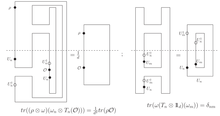
Figure 11: All tight teleportation and dense coding schemes.

A note is added for a characteristic equation for the dense coding. As Alice and Bob share the maximally entangled state $|\Omega\rangle_{AB}$, Alice transforms her state by the local unitary transformation $T_{n}$ to encode a message $n$ and then Bob performs the measurement on an observable $\omega_{m}$ of his system. In the case of $n=m$, Bob gets the message. All the tight dense coding schemes are concluded in the equation,

$$tr(\omega(T_{n}\otimes 1\!\!1_{d})(\omega_{m}))=\delta_{nm}$$ (49)

which can be proved in our diagrammatic approach, see the right term of Figure 11.

4 Generalized Temperley–Lieb configurations

Diagrammatical tricks involved in Figure 11 for deriving characteristic equations for all tight teleportation and dense coding schemes, shed us an insight that our diagrammatical quantum circuits have topological features to be explained by a mathematical structure. The diagrammatic representation for the teleportation based on quantum measurements, Figure 10 is a key clue for us because it is a standard configuration for the product $E_{1}E_{2}$ of the Temperley–Lieb algebra as the local unitary transformation $U_{n}$ is an identity.

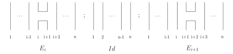
Figure 12: The $TL_{n}$ generators $E_{i}$, $Id$ and $E_{i+1}$.

We propose the Temperley–Lieb algebra under local unitary transformations to be a suitable algebraic structure underlying the teleportation. The Temperley–Lieb algebra $TL_{n}(\lambda)$ is generated by the identity $Id$ and $n-1$ hermitian projectors $E_{i}$ satisfying

$$E_{i}^{2} = E_{i},\qquad(E_{i})^{\dagger}=E_{i},\,\,\,i=1,\ldots,n-1,$$

$$E_{i}E_{i\pm 1}E_{i} = \lambda^{-2}E_{i},\qquad E_{i}E_{j}=E_{j}E_{i},\,\,\,|i-j|>1,$$ (50)

in which $\lambda$ is called the loop parameter. The diagrammatical representation for the Temperley–Lieb algebra $TL_{n}(\lambda)$, called the Brauer diagram [44] or Kauffman diagram [46, 47] in literature, consists of planar diagrams $(n,n)$ that make connections between two rows of $n$ points. Each point in the top row is connected to another different point in the top or bottom row by an arc, but all arcs in a diagram have to be disjoint of each other.

See Figure 12. The identity $Id$ is represented by a diagram with $n$ parallel vertical strings. A diagrammatical representation for the idempotent $E_{i}$ is similar to the diagram for the identity $Id$ except that the $i$th and $i+1$th top (and bottom) points are connected. A diagram for the idempotent $E_{i+1}$ is obtained in the same way. Here the configurations of cups and caps appear and they are formed by connecting different points in the same row: A cup (cap) refers to an arc between two distinct points at the top (bottom) row.

Hence our diagrammatical rules take roots in the diagrammatical representation for the Temperley-Lieb algebra. The reason is that the maximally entangled state $\omega$ can form a representation of the $TL_{n}(d)$ algebra with the loop parameter $d$. For example, the $TL_{3}(d)$ algebra is generated by two idempotents $E_{1}$ and $E_{2}$ given by

$$E_{1}=\omega\otimes Id,\qquad E_{2}=Id\otimes\omega,$$ (51)

which satisfy the axiom $E_{1}E_{2}E_{1}=\frac{1}{d^{2}}E_{1}$ in the way

$$E_{1}E_{2}E_{1}|\alpha\beta\gamma\rangle=\frac{1}{d}\sum_{l=0}^{d-1}E_{1}E_{2}|ll\gamma\rangle\delta_{\alpha\beta}=\frac{1}{d^{3}}\sum_{n=0}^{d-1}|nn\gamma\rangle\delta_{\alpha\beta}=\frac{1}{d^{2}}E_{1}|\alpha\beta\gamma\rangle$$ (52)

and satisfy the axiom $E_{2}E_{1}E_{2}=\frac{1}{d^{2}}E_{2}$ via a similar calculation.

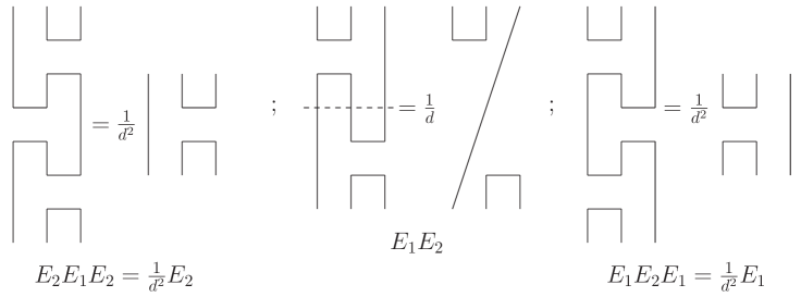
Figure 13: The diagrammatical representation for the $TL_{3}(d)$ algebra.

See Figure 13. The product $E_{i}E_{j}$ of $E_{i}$ and $E_{j}$ is a tangle product obtained by attaching bottom points of $E_{i}$ to top points of $E_{j}$. A resulted diagram may have loops which have an interpretation in terms of the loop number $\lambda$. A diagram for the product $E_{i}E_{i+1}$ ($E_{i+1}E_{i}$) is the same as Figure 9 except those points representing local unitary transformations, and so it is called the teleportation configuration in our paper.

See Figure 13 again. We can set up the $TL_{3}(d)$ algebra in terms of our diagrammatical rules by diagrammatically proving the axioms that the idempotents $E_{1}$ and $E_{2}$ (51) have to satisfy. The diagrammatical proof applies topological diagrammatical operations by straightening configurations of cups and caps into a straight line. Such diagrammatical tricks have been exploited in the derivation of characteristic equations for all tight teleportation and dense coding schemes in Figure 10. Note that each cup (cap) is with a normalization factor $d^{-\frac{1}{2}}$. The normalization factor $\frac{1}{d}$ in the teleportation configuration $E_{1}E_{2}$ is from vanishing of a cup and cap, while the normalization factor $\frac{1}{d^{2}}$ in $E_{1}E_{2}E_{1}$ is from four vanishing cups and caps.

In terms of the density matrix $\omega_{n}$ (37) which is a local unitary transformation of the maximally entangled state $\omega$, we can set up a representation of the Temperley–Lieb algebra $TL_{n}(d)$. For example, the $TL_{3}(d)$ algebra can be generated by $\tilde{E}_{1}$ and $\tilde{E}_{2}$,

$$\tilde{E}_{1}=\omega_{n}\otimes Id,\qquad\tilde{E}_{2}=Id\otimes\omega_{n},$$ (53)

which are proved to satisfy the axioms of the Temperley–Lieb algebra in our diagrammatic approach. See Figure 14. Therefore we think that these configurations, devised for quantum information protocols involving maximally entangled states, projective measurements and local unitary transformations, belong to our generalized Temperley–Lieb configurations, i.e., Temperley-Lieb diagrams with solid points or small circles in our diagrammatic approach. That is to say that we propose the Temperley–Lieb algebra under local unitary transformations to underlie the quantum teleportation phenomena.

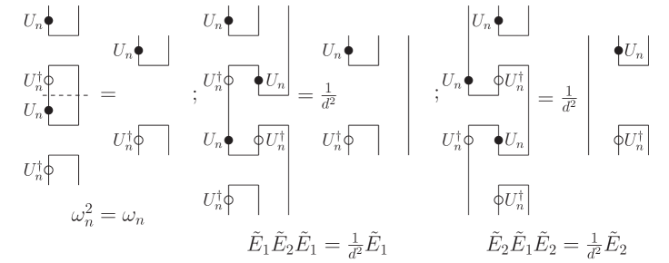
Figure 14: The $TL_{3}(d)$ algebra under local unitary transformations.

The teleportation configuration $E_{i}E_{i+1}$ ($E_{i+1}E_{i}$) is a product of two idempotents $E_{i}$ and $E_{i+1}$. Here we explain it to be a fundamental configuration for defining the Brauer algebra $D_{n}(\lambda)$ which is an extension of the Temperley–Lieb algebra $TL_{n}(\lambda)$ with virtual crossings. The Temperley-Lieb idempotents $E_{i}$ and virtual crossings $v_{i}$ (2.2) have to satisfy the following mixed relations:

$$E_{i}v_{i}=v_{i}E_{i}=E_{i},\qquad E_{i}v_{j}=v_{j}E_{i},\qquad j\neq i\pm 1,i=1,\cdots,n-1,$$

$$v_{i\pm 1}v_{i}E_{i\pm 1}=\lambda E_{i}E_{i\pm 1},\qquad\,\,\,E_{i}v_{i\pm 1}v_{i}=\lambda E_{i}E_{i\pm 1}.$$ (54)

See Figure 15. The axiom that the teleportation configuration $E_{i}E_{i+1}$ ($E_{i+1}E_{i}$) is equivalent to the configuration $v_{i+1}v_{i}E_{i+1}$ ($v_{i}v_{i+1}E_{i}$) informs us that the teleportation can be performed via two quantum gates denoted by a virtual crossing $v$ and the Bell measurement denoted by an idempotent $E$. For example, with the permutation $P$ (18) as a virtual crossing and the maximally entangled state $\omega$ as an idempotent, they form a representation of the Brauer algebra $D_{2}(d)$ with the loop parameter $d$, see [23] for the detail where $\omega$ is regarded as the partial transpose of permutation $P$. Hence it is interesting for quantum computing that the teleportation can be realized by two swap gates $P$ and the Bell measurement $\omega$.

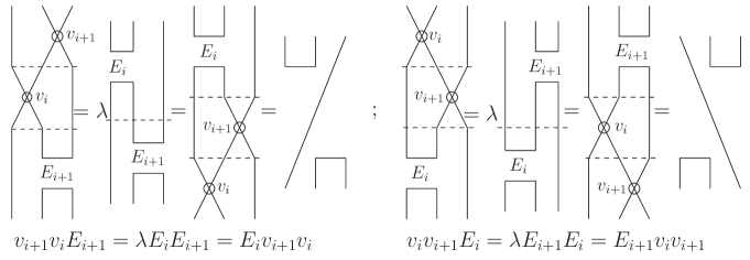
Figure 15: Teleportation, teleportation swapping and Brauer algebra.

5 Comparisons with known approaches

We propose the Temperley–Lieb algebra under local unitary transformations to be a right mathematical framework for the quantum teleportation phenomena. Here we compare it with two known approaches to the quantum information flow: the teleportation topology [11, 21] and strongly compact closed category theory [27], in order to emphasize essential differences among them.

5.1 Comparison with teleportation topology

Teleportation topology [11, 21] regards the teleportation as a kind of topological amplitude. There are one to one correspondences between quantum amplitudes and topological amplitudes. The state preparation (a Dirac ket) describes a creation of two particles from the vacuum and has a diagrammatic representation of a cup vector $|Cup\rangle$, while the measurement process (a Dirac bra) denotes an annihilation of two particles and is related to a cap vector $\langle Cap|$. The cup and cap vectors are associated with matrices $M$ and $N$ in the way,

$$|Cup\rangle=\sum_{i,j=0}^{d-1}M_{ij}|e_{i}\otimes e_{j}\rangle,\qquad\langle Cap|=\sum_{i,j=0}^{d-1}\langle e_{i}\otimes e_{j}|N_{ij}$$ (55)

which have to satisfy a topological condition, i.e., the concatenation of a cup and a cap is a straight line denoted by the identity matrix $N_{ij}M_{jk}=\delta_{ik}$. See Figure 16.

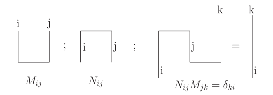
Figure 16: Teleportation topology: cup, cap and topological condition.

However, our diagrammatic rules does not admit an interpretation of the teleportation topology. First, the concatenation of a cup and a cap is formulated via the concept of the transfer operator (33) which is not an identity required by the topological condition. Second, our cup and cap vectors are normalized maximally entangled vectors given by

$$|Cup\rangle=\frac{1}{\sqrt{d}}\sum_{i=0}^{d-1}|e_{i}\otimes e_{i}\rangle,\qquad\langle Cap|=\frac{1}{\sqrt{d}}\sum_{i=0}^{d-1}\langle e_{i}\otimes e_{i}|$$ (56)

which leads to a normalization factor $\frac{1}{d}$ to the straight line from the concatenation of a cup and a cap. Third, our approach underlies the Temperley–Lieb configurations and so involves all kinds of combinations of cups and caps. For example, a projector is represented by a top cup with a bottom cap, as is not considered by the teleportation topology.

5.2 Quantum information flow in the categorical approach

We set up one to one correspondences between a bipartite vector and a map. There are a $d_{1}$-dimension Hilbert space ${\cal H}_{(1)}$ and a $d_{2}$-dimension Hilbert space ${\cal H}_{(2)}$. A bipartite vector $|\Phi\rangle$ has a form in terms of product bases $|e^{(1)}_{i}\rangle\otimes|e^{(2)}_{j}\rangle$ of ${\cal H}_{(1)}\otimes{\cal H}_{(2)}$,

$$|\Phi\rangle=\sum_{i=0}^{d_{1}-1}\sum_{j=0}^{d_{2}-1}m_{ij}|e^{(1)}_{i}\rangle\otimes|e^{(2)}_{j}\rangle,\qquad\langle\Phi|=\sum_{i=0}^{d_{1}-1}\sum_{j=0}^{d_{2}-1}m^{\ast}_{ij}\langle e^{(1)}_{i}|\otimes\langle e^{(2)}_{j}|$$ (57)

where $\langle\Phi|$ denotes a dual vector of $|\Phi\rangle$ in a dual product space ${\cal H}^{\ast}_{(1)}\otimes{\cal H}^{\ast}_{(2)}$ with the basis $\langle e^{(1)}_{i}|\otimes\langle e^{(2)}_{j}|$. As the product bases are fixed the bipartite vectors $|\Phi\rangle$ or $\langle\Phi|$ are also determined by a $d_{1}\times d_{2}$ matrix $M_{d_{1}\times d_{2}}=(m_{ij})$. Define two types of maps $f$ and $f^{\ast}$ in the way,

$$f:{\cal H}_{1}\rightarrow{\cal H}^{\ast}_{2},\qquad f(\cdot)=\sum_{i=0}^{d_{1}-1}\sum_{j=0}^{d_{2}-1}m_{ij}\langle e^{(1)}_{i}|\cdot\rangle\langle e^{(2)}_{j}|,$$

$$f^{\ast}:{\cal H}^{\ast}_{1}\rightarrow{\cal H}_{2},\qquad f^{\ast}(\cdot)=\sum_{i=0}^{d_{1}-1}\sum_{j=0}^{d_{2}-1}m_{ij}|e^{(2)}_{j}\rangle\langle\cdot|e^{(1)}_{i}\rangle.$$ (58)

We have the following bijective correspondences,

$$|\Phi\rangle\approx\langle\Phi|\approx M\approx f\approx f^{\ast}$$ (59)

which suggests that we can label a bipartite project $|\Phi\rangle\langle\Phi|$ by the map $f$ or $f^{\ast}$ or matrix $M$.

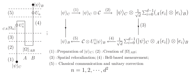
Figure 17: Quantum information flow and strongly compact closed category.

To transport Charlie’s unknown quantum state $|\psi\rangle_{C}$ to Bob, the teleportation has to complete all the operations: preparation of $|\psi\rangle_{C}$; creation of $|\Omega\rangle_{AB}$ in Alice and Bob’s systems; Bell-based measurement ${}_{CA}\langle\Omega_{n}|$ in Charlie and Alice’s systems; classical communication between Alice and Bob; Bob’s local unitary correction. These steps divide the quantum information flow into six pieces which are shown in the left term of Figure 17 where the third piece represents a process bringing Alice and Charlies’ particles together for an entangling measurement. In the category theory, every step or piece is denoted by a specific map which satisfies the axioms of the strongly compact closed category theory. The crucial point is to identify a bijective correspondence between the Bell vector and a map from the dual Hilbert space ${\cal H}^{\ast}$ to the Hilbert space $\cal H$, i.e.,

$$\frac{1}{\sqrt{d}}\sum_{i=0}^{d-1}|e_{i}\rangle_{A}\otimes|e_{i}\rangle_{B}\approx\frac{1}{\sqrt{d}}\sum_{i=0}^{d-1}{}_{A}\langle e_{i}|\otimes|e_{i}\rangle_{B},\qquad{\cal H}_{A}\otimes{\cal H}_{B}\approx{\cal H}_{A}^{\ast}\otimes{\cal H}_{B}$$ (60)

so that the strongly compact closed category theory has a physical realization in the form of the quantum information flow. See the right term of Figure 17 where the symbol ${\mathcal{C}}$ denotes the complex field and we have

$$|\psi\rangle_{C}\approx|\psi\rangle_{C}\otimes{\mathcal{C}},\qquad|\psi\rangle_{B}\approx{\mathcal{C}}\otimes|\psi\rangle_{B},$$ (61)

and we can create a bipartite state from a complex number ${\mathcal{C}}$ and also annihilate it into ${\mathcal{C}}$. Note that the appearance of ${\cal H}^{\ast}\otimes{\cal H}$ is not require by the teleportation or the quantum information flow but is imposed by the axioms of the strongly compact closed category theory.

To sketch the quantum information flow in the form of compositions of a series of maps which are central topics of the category theory, we study an example in details. Set five Hilbert spaces ${\cal H}_{i}$ and its dual ${\cal H}^{\ast}_{i}$, $i=1,\cdots,5$ and define eight bipartite projectors $P_{\alpha}=|\Phi_{\alpha}\rangle\langle\Phi_{\alpha}|$, $\alpha=1,\cdots,8$ in which a bipartite vector $|\Phi_{\alpha}\rangle$ is an element of ${\cal H}_{i}\otimes{\cal H}_{i+1}$, $i=1,\cdots,4$. In the left diagram of Figure 18, every box represents a bipartite projector $P_{\alpha}$ and a vector $|\phi_{C}\rangle\in{\cal H}_{1}$ that Charlie owns will be transported to Bob who is supposed to obtain a vector $|\phi_{B}\rangle\in{\cal H}_{5}$ through the quantum information flow. The projectors $P_{1}$ and $P_{2}$ pick up an incoming vector in ${\cal H}_{2}\otimes{\cal H}_{3}\otimes{\cal H}_{4}\otimes{\cal H}_{5}$ and the projectors $P_{7}$ and $P_{8}$ determine an outgoing vector in ${\cal H}_{1}\otimes{\cal H}_{2}\otimes{\cal H}_{3}\otimes{\cal H}_{4}$. The right diagram in Figure 18 shows the quantum information flow from $|\phi_{C}\rangle$ to $|\phi_{B}\rangle$ in a clear way. It is drawn according to permitted and forbidden rules [28]: a flow is forbidden to go through a box from the one side to the other side, and is forbidden to be reflected at the incoming point, and has to change its direction from an incoming flow to an outgoing flow as it passes through a box. Obviously, if those rules are not imposed there will be many possible pathes from $|\phi_{C}\rangle$ to $|\phi_{B}\rangle$.

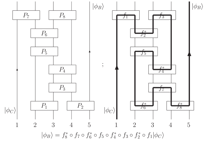
Figure 18: Quantum information flow in the categorical approach.

We now work out a formalism of the quantum information flow in the categorical approach. Consider the projector $P_{7}=|\Phi_{7}\rangle\langle\Phi_{7}|$ and introduce the map $f_{1}$ to represent the action of $\langle\Phi_{7}|$, a half of $P_{7}$,

$$f_{1}:{\cal H}_{1}\rightarrow{\cal H}_{2}^{\ast},\qquad f_{1}|\phi_{C}\rangle=\langle\Phi_{7}|\phi_{C}\rangle.$$ (62)

Similarly, the remaining seven boxes are labeled by the maps $f_{2}^{\ast}$, $f_{3}$, $f_{4}^{\ast}$, $f_{5}$, $f_{6}^{\ast}$, $f_{7}$ and $f_{8}^{\ast}$, respectively and so the quantum information flow is encoded in the the form of a series of maps,

$$|\phi_{B}\rangle=f_{8}^{\ast}\circ f_{7}\circ f_{6}^{\ast}\circ f_{5}\circ f_{4}^{\ast}\circ f_{3}\circ f_{2}^{\ast}\circ f_{1}|\phi_{C}\rangle$$ (63)

where we identify the tensor product $|\Phi\rangle\otimes 1\!\!1_{d}\otimes\cdots\otimes 1\!\!1_{d}$ with $|\Phi\rangle$. Additionally, following rules of the teleportation topology [11, 21] and assigning the matrices $M,N$ to a cup and a cap respectively, we have the quantum information flow in the matrix teleportation,

$$|\phi_{B}\rangle=M_{8}\cdot N_{7}\cdot M_{6}\cdot N_{5}\cdot M_{4}\cdot N_{3}\cdot M_{2}\cdot N_{1}|\phi_{C}\rangle.$$ (64)

5.3 Comparisons with the categorical approach

We make conceptual differences clear between our diagrammatic teleportation approach and the categorical description for quantum information flow. They are essential: both physical and mathematical. In the mathematical side, we believe the braid group and Temperley–Lieb algebra underlying the teleportation instead of various maps in the category theory because we seek for a real bridge between knot theory and quantum information [23]. A bipartite projector is an idempotent of the Temperley–Lieb algebra but in the categorical approach only its half, a bipartite vector, is exploited. In the physical side, we use concepts like the Hilbert space, state, vector and local unitary transformation which are basic ingredients of standard quantum mechanics described by the von Neummann’s axioms, while the categorical approach aims at setting up a high-level approach beyond the von Neummann’s axioms.

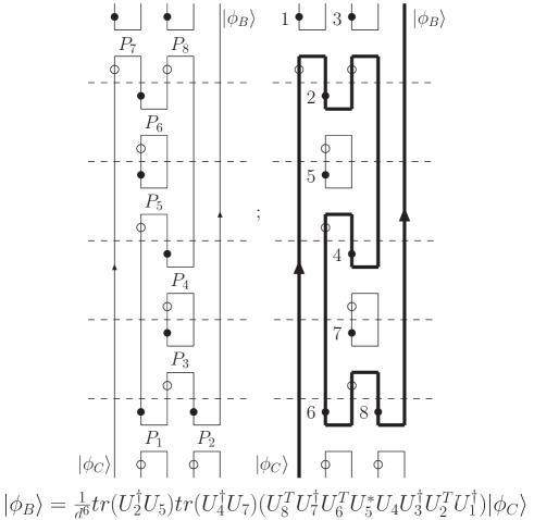
Figure 19: Quantum information flow in the Temperley–Lieb configurations.

To explain these differences in the detail, we revisit the example in Figure 18 and redraw a diagram according to our diagrammatical rules. In Figure 19, every projector consists of a top cup and a bottom cap denoting maximally entangled vectors $|\Omega\rangle$ and $\langle\Omega|$. The solid points $1,\cdots 8$ on the left branches of cups denote local unitary transformations $U_{1},\cdots,U_{8}$ and small circles on the left branches of caps denote their adjoint operators $U_{1}^{\dagger},\cdots,U_{8}^{\dagger}$, respectively. Following our rules, a quantum information flow from $|\phi_{C}\rangle$ to $|\phi_{B}\rangle$ is determined by the transfer operator given by

$$|\phi_{B}\rangle=\frac{1}{d^{6}}tr(U_{2}^{\dagger}U_{5})tr(U_{4}^{\dagger}U_{7})(U_{8}^{T}U_{7}^{\dagger}U_{6}^{T}U_{5}^{\ast}U_{4}U_{3}^{\dagger}U_{2}^{T}U_{1}^{\dagger})|\phi_{C}\rangle$$ (65)

where the normalization factor $\frac{1}{d^{6}}$ is contributed from six vanishing cups and six vanishing caps, and two traces are representations of two closed circles.

There are several remarkable things to be mentioned as Figure 18 is compared with Figure 19. Our diagrammatical approach not only derives the quantum information flow from $|\phi_{C}\rangle$ to $|\phi_{B}\rangle$ in a natural way but also yields a normalization factor from the closed circles. This normalization factor is crucial for the quantum formation flow. For examples, setting eight local unitary operators $U_{i}$ to be an identity leads to $|\phi_{B}\rangle=\frac{1}{d^{4}}|\phi_{C}\rangle$, or assuming $U_{2}$ and $U_{5}$ (or $U_{4}$ and $U_{7}$) orthogonal to each other gives a zero vector, i.e., $|\phi_{B}\rangle=0$, no flow!

About the acausality problem which arises in the description for the quantum information flow, we think that it is not reasonable to argue such a question on the teleportation without considering the whole process from the global view. See Figure 18 and Figure 19: the quantum information flow is only one part of the diagram in our diagrammatical approach. Note that in the categorical approach the quantum information flow is created under the guidance of additional permitted and forbidden rules [28] but in our approach it is derived in a natural way without any imposed rules, as can be observed in the comparison of Figure 18 with Figure 19.

Furthermore, we can apply a bijective correspondence between a local unitary transformation and a bipartite vector, as is different from a choice preferred by the categorical approach. For example, we have

$$|\psi(U)\rangle=(U\otimes 1\!\!1_{d})|\Omega\rangle,\qquad|\psi(U)\rangle\approx U\approx|\psi(U)\rangle\langle\psi(U)|$$ (66)

and so the Bell states (2.1) are represented by an identity or the Pauli matrices

$$|\phi^{+}\rangle\approx 1\!\!1_{2},\,\,\,|\phi^{-}\rangle\approx\sigma_{3},\,\,\,|\psi^{+}\rangle\approx\sigma_{1},\,\,\,|\psi^{-}\rangle\approx i\sigma_{2}.$$ (67)

Hence we can regard the equation (65) as the quantum information flow in terms of local unitary transformations.

6 Concluding remarks and outlooks

In this paper, we apply the braid group, Temperley–Lieb algebra and Brauer algebra to mathematical descriptions of the quantum teleportation phenomena. As a remark, we explore the virtual braid structure in the teleportation equation, and propose the braid teleportation configuration $(b^{-1}\otimes Id)(Id\otimes b)$. They are expected to be related to the braid statistics of anyons or topological quantum computing [48]. We will make a further study on the connection between the braid teleportation configuration and crossed measurement [41].

In our further research [49, 50], we explore the braid teleportation configuration $(b^{-1}\otimes Id)(Id\otimes b)$ in the state model [8] which is devised for a braid representation of the Temperley–Lieb algebra and applied to a disentanglement of a knot or link. We find that the braid teleportation configuration consists of teleportation and non-teleportation terms and realize that the teleportation term is a basic element of the Temperley–Lieb algebra. In addition, we study new types of quantum algebras via the RTT relation of the Bell matrix [51, 52].

We design diagrammatic rules for quantum information protocols involving maximally entangled states, and apply them to three different types of descriptions for the teleportation: the transfer operator [43]; quantum measurements [40, 41, 42]; characteristic equations for tight teleportation schemes [22]. The tight teleportation scheme includes all elements of the teleportation and unifies them from the global view into an algebraic or diagrammatic equation, while the other approaches such as the standard description [7], the transfer operator [43] and quantum measurements [41], all observe the teleportation from the local point of view.

Based on our diagrammatical representations for various descriptions of the quantum teleportation phenomena, we propose the Temperley–Lieb algebra under local unitary transformations to be an algebraic structure underlying quantum information protocols involving maximally entangled states, projective measurements and local unitary transformations. We find the teleportation configuration to be a fundamental element for defining the Brauer algebra and obtain an equivalent realization of the teleportation in terms of swap gates and Bell measurements.

In the extension of the present paper [49, 50], we apply our diagrammatical rules to the entanglement swapping [53], quantum computing [54] and multi-partite entanglements. The entanglement swapping yields an entangled state between two systems which never met before and have no physical interactions, and it has a characteristic equation which can be derived in our diagrammatical approach. In the quantum computing which chooses the teleportation as a primitive element, we show the Temperley–Lieb configurations for a unitary braid gate, swap gate and CNOT gate. Additionally, we discuss how to represent multipartite entangled states in our diagrammatic approach.

In a general sense, Bell measurements and local unitary transformations are crucial points for an application of our diagrammatic rules. We expect our diagrammatic approach to be exploited in topics such as Bell inequalities, quantum cryptography, and so on. To develop our diagrammatical rules, we refer to the work on atemporal diagrams for quantum circuits [55] where a system of diagrams is introduced for the representation of various elements of a quantum circuit in a form which makes no reference to time. Note that our diagrammatical rules are devised for uncovering topological features in quantum circuits but an atemporal diagram is a kind of diagrammatical notation for a quantum circuit.

In our further research, we will continue to explore applications of mathematical structures involved in this paper. We expect the categorical theory to play important roles in the study of the quantum information phenomena in view of [29, 34, 56, 57, 58]. We think that the Temperley–Lieb algebra under local unitary transformations, is an interesting mathematical subject, because it contains abundant mathematical objects such as braids and provides a kind of realization of quantum computing. As a virtual braid representation can be obtained via the Brauer algebra (i.e., the virtual Temperley–Lieb algebra [23, 59]), we need set up connections between the virtual braid teleportation configuration and virtual Temperley–Lieb configuration.

References

- [1] R.F. Werner, Quantum States with Einstein-Podolsky-Rosen Correlations Admitting a Hidden-Variable Model, Phys. Rev. A 40 (1989) 4277.
- [2] M. Nielsen and I. Chuang, Quantum Computation and Quantum Information (Cambridge University Press, 1999).
- [3] P.W. Shor, Algorithms for Quantum Computation: Discrete Logrithms and Factoring. In S. Goldwasser, editor, Proceedings of the 35th Annual Symposium on the Foundations of Computer Science, pp. 124-134, Los Alamitos, CA, 1994. IEEE Computer Society Press.
- [4] L.K. Grover, Quantum Mechanics Helps in Searching for a Needle in a Haystack, Phys. Rev. Lett. 78 (1997) 325-328.
- [5] C.H. Bennett, G. Brassard, Quantum Cryptography: Public Key Distribution and Coin Tossing, Int. Conf. Computers, Systems & Signal Processing, Bangalore, India, December 10-12, 1984, pp. 175-179.
- [6] A.K. Ekert, Quantum Cryptography Based on Bell’s Theorem, Phys. Rev. Lett. 67 (1991) 661-663.
- [7] C.H. Bennett, G. Brassard, C. Crepeau, R. Jozsa, A. Peres and W. K. Wootters, Teleporting an Unknown Quantum State via Dual Classical and Einstein-Podolsky-Rosen Channels, Phys. Rev. Lett. 70 (1993) 1895-1899.
- [8] L.H. Kauffman, Knots and Physics (World Scientific Publishers, 2002).
- [9] J.L. Brylinski and R. Brylinski, Universal Quantum Gates, in Mathematics of Quantum Computation, Chapman & Hall/CRC Press, Boca Raton, Florida, 2002 (edited by R. Brylinski and G. Chen).
- [10] H.A. Dye, Unitary Solutions to the Yang–Baxter Equation in Dimension Four, Quant. Inf. Proc. 2 (2003) 117-150. Arxiv: quant-ph/0211050.
- [11] L.H. Kauffman and S.J. Lomonaco Jr., Braiding Operators are Universal Quantum Gates, New J. Phys. 6 (2004) 134. Arxiv: quant-ph/0401090.
- [12] Y. Zhang, L.H. Kauffman and M.L. Ge, Universal Quantum Gate, Yang–Baxterization and Hamiltonian. Int. J. Quant. Inform., Vol. 3, 4 (2005) 669-678. Arxiv: quant-ph/0412095.
- [13] Y. Zhang, L.H. Kauffman and M.L. Ge, Yang–Baxterizations, Universal Quantum Gates and Hamiltonians. Quant. Inf. Proc. 4 (2005) 159-197. Arxiv: quant-ph/0502015.
- [14] C.N. Yang, Some Exact Results for the Many Body Problems in One Dimension with Repulsive Delta Function Interaction, Phys. Rev. Lett. 19 (1967) 1312-1314.
- [15] R.J. Baxter, Partition Function of the Eight-Vertex Lattice Model, Annals Phys. 70 (1972) 193-228.
- [16] L.H. Kauffman, Quantum Computation and the Jones Polynomial, in Quantum Computation and Information, S. Lomonaco, Jr. (ed.), AMS CONM/305, 2002, pp. 101-137. Arxiv: math. QA/0105255.
- [17] L.H. Kauffman, Quantum Topology and Quantum Computing, in Quantum Computation, S. Lomonaco (ed.), AMS PSAPM/58, 2002, pp. 273–303.
- [18] L. H. Kauffman and S. J. Lomonaco Jr., Quantum Knots, in E. Donkor, A.R. Pirich and H.E. Brandt (eds.), Quantum Information and Computation II, Spie Proceedings, (12 -14 April, Orlando, FL, 2004), Vol. 5436, pp. 268-284. Arxiv: quant-ph/0403228.
- [19] L.H. Kauffman and S.J. Lomonaco Jr., Quantum Entanglement and Topological Entanglement, New J. Phys. 4 (2002) 73.1–73.18.
- [20] L.H. Kauffman and S.J. Lomonaco Jr., Entanglement Criteria–Quantum and Topological, in E. Donkor, A.R. Pirich and H.E. Brandt (eds.), Quantum Information and Computation – Spie Proceedings, (21-22 April, Orlando, FL, 2003), Vol. 5105, pp. 51-58. Arxiv: quan-ph/0304091.
- [21] L.H. Kauffman, Teleportation Topology. Opt. Spectrosc. 9 (2005) 227-232. Arxiv: quan-ph/0407224.
- [22] R. F. Werner, All Teleportation and Dense Coding Schemes, J. Phys. A 35 (2001) 7081–7094. Arxiv: quant-ph/0003070.
- [23] Y. Zhang, L.H. Kauffman and R.F. Werner, Permutation and its Partial Transpose. Arxiv: quant-ph/0606005. Accepted by International Journal of Quantum Information for publication.
- [24] H.N.V. Temperley and E.H. Lieb, Relations between the ‘Percolation’ and ‘Colouring’ Problem and Other Graph-Theoretical Problems Associated with Regular Planar Lattices: Some Exact Results for the ‘Percolation’ Problem, Proc. Roy. Soc. A 322 (1971) 251-280.
- [25] S. Abramsky, and B. Coecke, Physical Traces: Quantum vs. Classical Information Processing. Electronic notes on Theoretical Computer Science 69 (special issue: Proceedings of Category Theory in Computer Science 2002). Arxiv:cs/0207057.
- [26] S. Abramsky, and B. Coecke, Abstract Physical Traces. Theory and Applications of Categories 14 (2003) 111–124.
- [27] B. Coecke, The Logic of Entanglement. An Invitation. Oxford University Computing Laboratory Research Report nr. PRG-RR-03-12. An 8 page short version is at Arxiv:quant-ph/0402014. The full 160 page version is at web.comlab.ox.ac.uk/oucl/ publications/tr/rr-03-12.html.
- [28] B. Coecke, Quantum Information-Flow, Concretely, and Axiomatically. In: Proceedings of Quantum Informatics 2004, pp. 15–29, Y. I. Ozhigov, Ed., Proceedings of Spie, Vol. 5833. Arxiv:quant-ph/0506132.
- [29] S. Abramsky, and B. Coecke, A Categorical Semantics of Quantum Protocols. In: Proceedings of the 19th Annual IEEE Symposium on Logic in Computer Science (LiCS‘04), IEEE Computer Science Press. Arxiv:quant-ph/0402130.
- [30] B. Coecke, De-linearizing Linearity: Projective Quantum Axiomatics from Strong Compact Closure. Electronic Notes in Theoretical Computer Science (special issue: Proceedings of the 3rd International Workshop on Quantum Programming Languages). Arxiv:quant-ph/0506134.
- [31] B. Coecke, Kindergarten Quantum Mechanic–Leture Notes. In: Quantum Theory: Reconstructions of the Foundations III, pp. 81-98, A. Khrennikov, American Institute of Physics Press. Arxiv: quant-ph/0510032.
- [32] B. Coecke, Introducing Categories to the Practicing Physicist, in What is Category Theory? Advanced Studies in Mathematics and Logic 30, pp. 45-74, Polimetrica Publishing, 2005.
- [33] B. Coecke and D. Pavlovic, Quantum Measurements Without Sums, to appear in: Mathematics of Quantum Computing and Technology.
- [34] S. Abramsky and R. Duncan, A Categorical Quantum Logic. Arxiv: quant-ph/0512114.
- [35] S. Abramsky, High-Level Methods for Quantum Computation and Quantum Information. Pleanary talk at 19th Annual IEEE Symposium on Logic in Computer Science (LiCS’04). Proceedings of the 19th Annual IEEE Symposium on Logic in Computer Science, IEEE Computer Science Press.
- [36] L.H. Kauffman, Virtual Knot Theory, European J. Comb. 20 (1999) 663-690.
- [37] L. H. Kauffman, A Survey of Virtual Knot Theory, in “Proceedings of Knots in Hellas 98” (World Scientific, Singpore, 2000) 143-202.
- [38] L. H. Kauffman, Detecting Virtual Knots, Atti. Sem. Mat. Fis. Univ. Modena, Supplemento al Vol. IL (2001) 241-282.
- [39] S. Kamada, Braid Representation of Virtual Knots and Welded Knots, Arxiv: math. GT/0008092.
- [40] Y. Aharonov, D.Z. Albert, and L. Vaidman, Measurement Process in Relativistic Quantum Theory, Phys. Rev. D 34 (1986) 1805-1813.
- [41] L. Vaidman, Teleportation of Quantum States, Phys. Rev. A 49 (1994) 1473-1475.
- [42] L. Vaidman, Instantaneous Measurement of Nonlocal Variables, Phys. Rev. Lett. 90 (2003) 010402
- [43] J. Preskill, Quantum Information and Computation, Lecture Notes for Ph219/CS219, Chapter 4, pp. 26-35. See http://www.iqi.caltech.edu/ presill/ph219.
- [44] R. Brauer, On Algebras Which are Connected With the Semisimple Continuous Groups, Ann. of Math. 38 (1937) 857-872.
- [45] N. Erez, Teleportation from a Projection Operator Point of View. Arxiv: quant-ph/0510130.
- [46] L.H. Kauffman and S.L. Lin, Temperley–Lieb Recoupling Theory and Invariants of Three-Manifold, Ann. of Math. Stud. 114 (Princeton Univ. Press, 1994).
- [47] L.H. Kauffman, Knot Diagrammatics, in W. Menasco and M. Thistlethwaite (eds.), Handbook of Knot Theory, (Elsevier, 2005), pp. 233–318. Arxiv: math. GN/0410329.
- [48] F. Wilczek, Fractional Statistics and Anyon Superconductivity (World Scientific, 1990).
- [49] Y. Zhang, Algebraic Structures Underlying Quantum Information Protocols. Note that it is an original version of the present manuscript. Arxiv: quant-ph/0601050.
- [50] Y. Zhang, Teleportation Braid Configuration and Temperley–Lieb Algebra, (in preparation).
- [51] Y. Zhang, N.H. Jing and M.L. Ge, New Quantum Algebras Associated with Bell States. Arxiv: math-ph/0610036.
- [52] J. Franko, E.C. Rowell and Z.H. Wang, Extraspecial 2-Groups and Images of Braid Group Representations. Arxiv: math.RT/0503435.
- [53] M. Żukowski, A. Zeilinger, M.A. Horne and A.K. Ekert, ‘Event-Ready-Detectors’ Bell Experiment via Entanglement Swapping. Phys. Rev. Let. 71 (1993) 4287–4290.
- [54] D. Gottesman and I.L. Chuang, Quantum Teleportation is a Universal Computational Primitive. Nature 402 (1999) 390–393. Arxiv:quant-ph/9908010.
- [55] R.B. Griffiths, S. Wu, L. Yu and S.M. Cohen, Atemporal Diagrams for Quantum Circuits, Phys. Rev. A 73 (2006) 052309. Arxiv: quant-ph/0507215.
- [56] J. Baez, Quantum Quandaries: A Category-Theoretic Perspective. In: S. French et al. (Eds.) Structural Foundations of Quantum Gravity, Oxford University Press. Arxiv:quant-ph/0404040.
- [57] P. Selinger, Dagger Compact Closed Categories and Completely Positive Maps. Electronic Notes in Theoretical Computer Science (special issue: Proceedings of the 3rd International Workshop on Quantum Programming Languages).
- [58] L.H. Kauffman and S.J. Lomonaco Jr., -Deformed Spin Networks, Knot Polynomials and Anyonic Topological Quantum Computation. Arxiv: quant-ph/0606114.
- [59] Y. Zhang, L.H. Kauffman and M.L. Ge, Virtual Extension of Temperley–Lieb Algebra, (in preparation).