Microscopic derivation of the Jaynes-Cummings model with cavity losses

Abstract

In this paper we provide a microscopic derivation of the master equation for the Jaynes-Cummings model with cavity losses. We single out both the differences with the phenomenological master equation used in the literature and the approximations under which the phenomenological model correctly describes the dynamics of the atom-cavity system. Some examples wherein the phenomenological and the microscopic master equations give rise to different predictions are discussed in detail.

I Introduction

The Jaynes-Cummings (JC) model is the fundamental model for the quantum description of matter-light interaction JC . It describes the dynamics of a two-level atom strongly interacting with a single mode of the quantized radiation field in the rotating-wave approximation (RWA). This model has been extensively studied in the past three decades shore_review ; puribook . Purely quantum effects predicted by the model, such as Rabi oscillations and collapses and revivals of the atomic inversion operator, have been observed in the experiments both with microcavities haroche ; harocheRMP ; Walther and with trapped ion systems wineland .

In cavity quantum electrodynamics, the JC model describes the strong-coupling regime of micromasers and of one-atom lasers. A realistic description of these systems, however, must take into account the photon losses due to imperfect reflectivity of the cavity mirrors. Cavity losses have been described in the literature by means of a phenomenological master equation of the form

$$\dot{\rho}=-i\left[H_{JC},\rho\right]+\gamma\left(a\rho a^{\dagger}-\frac{1}{2}a^{\dagger}a\rho-\frac{1}{2}\rho a^{\dagger}a\right),$$ (1)

where $\rho$ is the density matrix of the atom-cavity system, $H_{JC}$ is the Jaynes-Cummings Hamiltonian, and $\gamma$ represents the rate of loss of photons from the cavity, and where we have put $\hbar=1$. The second term on the r.h.s. of Eq. (1) has been derived microscopically in the framework of a different physical problem, i.e., the one wherein the system is given by the quantized cavity mode only, losing excitations because of its interaction with the surrounding electromagnetic field in the vacuum state cohen_libro .

In this paper we will show that, when the system consists not only of the cavity mode, but also of the two-level atom interacting with the cavity, the fully microscopic derivation gets more complicated, and in general the master equation for the atom-cavity system is not of the form given by Eq. (1). We will show that only under certain conditions the phenomenological master equation coincides with the microscopic one. These conditions are typically met in the cavity QED experiments, and this explains the extensive and successful use of Eq. (1) for the description of the dynamics of the JC model with losses. The knowledge of the limitations of the phenomenological model, however, allows us on the one hand to point out some misuse of the model, e.g., for the study of the damping of highly excited quasi-classical states geaben . On the other hand it paves the way to the correct description of photon losses in the case of structured reservoirs, e.g. for photonic bandgap cavities. Moreover, our derivation brings to light the microscopic processes which occur in the open system dynamics, and therefore how decoherence and dissipation come into play.

The paper is structured as follows. In Sec. II we give a short review on the JC model and on the usual phenomenological description of losses in this model. In Sec. III we present the microscopic derivation of the JC model with cavity losses, for the general case of a $T$ temperature electromagnetic reservoir. In Sec. IV we describe the dynamics for the case of one initial excitation in the atom-cavity system, we solve the master equation and we compare it with the solution of the phenomenological model existing in the literature. In Sec. V we briefly discuss some situations in which the use of the microscopic model could lead to substantial differences compared to the phenomenological model, suggesting experimental situations in which such differences could be observed, and finally we present conclusions.

II The Jaynes-Cummings model and the phenomenological description of losses

Since its introduction, in 1963 JC , the JC model has been one of the most used models for the description of radiation-matter interaction in quantum optics shore_review , in particular in cavity quantum electrodynamics haroche , and in ion traps wineland . In this section we briefly review some of its features.

Let us consider a two-level atom and denote by $\left|g\right>$ and $\left|e\right>$ the ground and excited state, respectively. The energy separation between the two states is given by $\hbar\omega_{0}$, with $\omega_{0}$ the Bohr frequency. The resonant interaction between the atom and a mode of the electromagnetic field, in the RWA and in units of $\hbar$, is described by the following Hamiltonian JC :

$$H_{JC}=\frac{\,\omega_{0}}{2}\sigma_{z}+\omega_{0}\,a^{\dagger}a+\Omega\left(a\sigma_{+}+a^{\dagger}\sigma_{-}\right),$$ (2)

where $a^{\dagger}$ ($a$) is the creation (annihilation) operator of the mode, $\sigma_{-}=\left|g\right>\left<e\right|$, $\sigma_{+}=\left|e\right>\left<g\right|$, and $\sigma_{z}=\left|e\rangle\langle e\right|-\left|g\rangle\langle g\right|$.

It is straightforward to show that the total number of excitations in the atom-cavity system, given by ${\cal N}=\left<a^{\dagger}a+\sigma_{z}+1/2\right>$, is a constant of motion. This allows to diagonalize easily the Hamiltonian $H_{JC}$. One finds the following eigenstates and eigenvalues shore_review :

$$\left|E_{N,\pm}\right>=\frac{1}{\sqrt{2}}\left(\left|N,g\right>\pm\left|N-1,e\right>\right),$$

$$E_{N,\pm}=\left(N-\frac{1}{2}\right)\omega_{0}\pm\Omega\sqrt{N},$$ (3)

for $N\geq 1$, while the ground state and the corresponding energy eigenvalue are

$$\left|E_{0}\right>=\left|0,g\right>,\hskip 28.45274ptE_{0}=-\frac{\omega_{0}}{2},$$ (4)

respectively, where $|N,i\rangle=|N\rangle|i\rangle$, with $i=e,g$, indicates the tensor product of the Fock state $|N\rangle$ and the electronic states $|i\rangle$.

From the eigenstates and the eigenvalues of $H_{JC}$ one can calculate the evolution of the system given any initial conditions. Well known examples of system dynamics are Rabi oscillations of the atomic state population, and collapses and revivals of the oscillations when the mode is initially in a coherent state shore_review .

In cavity quantum electrodynamics the main source of dissipation originates from the leakage of cavity photons due to imperfect reflectivity of the cavity mirrors. A second source of dissipation and decoherence, namely spontaneous emission of photons by the atom, is mostly suppressed by the presence of the cavity, and therefore its effect is usually neglected.

The dissipative dynamics of the quantized modes of the radiation field inside the cavity in absence of the atom, i.e., when the atom is not inside the cavity, can be derived microscopically assuming that the cavity modes are coupled with the electromagnetic field outside the cavity, which represents a reservoir at temperature $T$ cohen_libro . The typical approach to the description of the losses in the JC model consists in assuming that the presence of the atom inside the cavity does not modify strongly the mechanism of cavity losses, which therefore can be modelled by the above mentioned master equation. It is worth stressing further, however, that this approach is purely phenomenological, since it does not take into account, in the microscopic derivation, the presence of the atom inside the cavity. The phenomenological master equation has the form

$$\dot{\rho} = -i\left[H_{JC},\rho\right]$$ (5)

$$+ \gamma\left[n(\omega_{0})+1\right]\left[a\rho a^{\dagger}-\frac{1}{2}\left(a^{\dagger}a\rho+\rho a^{\dagger}a\right)\right]$$

$$+ \gamma n(\omega_{0})\left[a^{\dagger}\rho a-\frac{1}{2}\left(aa^{\dagger}\rho+\rho aa^{\dagger}\right)\right],$$

with $n(\omega_{0})$ the average number of quanta of the reservoir in the mode of frequency $\omega_{0}$, and $\gamma$ the rate of loss of cavity photons. We note that for a zero-$T$ reservoir the master equation above reduces to the one given by Eq. (1). Equations (1) and (5) have been assumed to be valid in most of the earlier studies dealing with the JC model with losses, for example in agar1 ; agar2 ; agar3 ; barnett ; briegel ; puribook ; harocheRMP .

The use of the master equations given by Eqs. (1) and (5) has also been motivated by the fact that in many cavity QED experiments the atoms fly through the cavity and actually remain inside the cavity only for a short time. This could induce one to think that the effect of their presence inside the cavity might be negligible. We believe, however, that a comparison with a microscopic master equation describing the coupling of the entire atom-cavity system with a reservoir of electromagnetic modes at $T$ temperature is highly desirable and it may both provide a justification of the validity of the phenomenological model under the typical experimental conditions and put into evidence the physical contexts where the use of such a model may be unjustified. This is the main motivation of the results we will describe in the following sections.

We begin, in the next section, by presenting the general formalism, reviewed, e.g., in Ref. petruccionebook , to derive a master equation for the open quantum system of interest starting from the microscopic Hamiltonian of the total closed system (system+environment). We will then compare the master equation we obtain with the one given by Eq. (5).

III Microscopic derivation of the quantum master equation

III.1 The general formalism

We assume that the open quantum system of interest, e.g., the atom-cavity system, is part of a larger system whose dynamics is unitary and governed by the Hamiltonian $H$. The external environment is that part of the total closed system other than the system of interest. The Hamiltonian of the total closed system is given by

$$H=H_{S}+H_{E}+H_{\rm int},$$ (6)

where $H_{S}$ and $H_{E}$, are the system and environment Hamiltonians, respectively, and $H_{\rm int}$ is the system-environment interaction Hamiltonian which is taken to be of the form

$$H_{\rm int}=A\otimes E,$$ (7)

with $A=A^{\dagger}$ and $E=E^{\dagger}$ Hermitian operators acting on the system and on the environment Hilbert spaces, respectively.

We expand the interaction Hamiltonian $H_{\rm int}$ by means of the relations

$$A = \sum_{\omega}A(\omega),$$

$$A(\omega) = \sum_{\epsilon^{\prime}-\epsilon=\omega}\Pi(\epsilon)A\Pi(\epsilon^{\prime}),$$ (8)

where $\Pi(\epsilon)$ is the projector onto the eigenspace corresponding to the eigenvalue $\epsilon$ of the operator $H_{S}$ and the sum is taken over all the Bohr frequencies relative to $H_{S}$.

Following the standard procedure, i.e., writing down the Liouville-von Neumann equation for the total density operator in the interaction picture with respect to $H_{S}+H_{E}$, performing the Born-Markov and the rotating wave approximations, tracing out the environmental degrees of freedom and then going back to the Schrödinger picture, one obtains the following master equation for the reduced density operator $\rho$ of the system petruccionebook :

$$\dot{\rho}(t)=-i[H_{S},\rho(t)]$$

$$+\sum_{\omega>0}\gamma(\omega)\left[A(\omega)\rho(t)A^{\dagger}(\omega)-\frac{1}{2}\left\{A^{\dagger}(\omega)A(\omega),\rho(t)\right\}\right]$$

$$+\!\!\!\!\sum_{\omega>0}\!\!\!\gamma(-\omega)\!\left[A^{\dagger}(\omega)\rho(t)A(\omega)\!-\!\frac{1}{2}\left\{A(\omega)A^{\dagger}(\omega),\rho(t)\right\}\right]\!,$$ (9)

where the relation $A(-\omega)=A^{\dagger}(\omega)$ has been used and where we have neglected the renormalization term petruccionebook . The coefficients $\gamma(\omega)$ are given by the Fourier transform of the correlation functions of the environment:

$$\gamma(\omega)=\int_{-\infty}^{+\infty}d\tau\,\mathrm{e}^{i\omega\tau}\left<E^{\dagger}(\tau)E(0)\right>,$$ (10)

where the environment operators are in the interaction picture.

We stress once more that the formalism presented above is valid as long as we can perform three approximations: weak coupling or Born approximation, Markovian approximation and rotating wave approximation. It is worth recalling that the Markovian approximation can be seen as a coarse-graining in time, and therefore holds as long as the correlation time of the reservoir $\tau$ is much smaller than the characteristic time scale of the system dynamics $t$

$$t\gg\tau.$$ (11)

The RWA, instead, is valid as long as the relaxation time of the system is much longer than the typical timescale of the free evolution of the quantum system, i.e., when the maximum of the rates $\gamma(\omega)$ is much smaller than the minimum difference between the Bohr frequencies relative to $H_{S}$ petruccionebook :

$$\gamma_{\rm max}\ll\Delta\omega_{\rm min}.$$ (12)

In the rest of this section we will apply this general formalism to the description of cavity losses in the Jaynes-Cummings model.

III.2 Application of the general formalism to the Jaynes-Cummings model

We model the environment as a collection of quantum harmonic oscillators in thermal equilibrium at $T$ temperature and we assume that the interaction Hamiltonian is linear in both the electromagnetic field of the cavity mode and the position operators of the harmonic oscillators, i.e.,

$$H_{S} = H_{JC},\;\;\;H_{E}=\sum_{k}\omega_{k}b^{\dagger}b,$$

$$H_{\rm int} = \left(a+a^{\dagger}\right)\sum_{k}g_{k}\left(b_{k}+b_{k}^{\dagger}\right),$$ (13)

with $\omega_{k}$ the frequencies of the environment oscillators, $b^{{\dagger}}_{k}$ ($b_{k}$) the creation (annihilation) operator of quanta in the $k$-th environmental mode, and $g_{k}$ the coupling constants.

For this system, the operators $A(\omega)$, defined in Eq. (III.1), are given by

$$A \!\!\!\left(\!E_{N^{\prime}\!,\,l}\!-\!E_{N,\,m}\right)=\left|E_{N,\,m}\right>\left<E_{N,\,m}\right|\!\left(a+a^{\dagger}\right)\!\left|E_{N^{\prime}\!,\,l}\right>\left<E_{N^{\prime}\!,\,l}\right|$$ (14)

$$= \frac{1}{2}\delta_{N,N^{\prime}-1}\!\left(\!\sqrt{N+1}+lm\sqrt{N}\right)\left|E_{N,\,m}\right>\left<E_{N+1,\,l}\right|,$$

for $N\geq 1$ and

$$A\left(E_{1,\pm}-E_{0}\right)=\frac{1}{\sqrt{2}}\left|E_{0}\right>\left<E_{1,\pm}\right|,$$ (15)

for $N=1$. In Eq. (14) we indicate the states $\left|E_{N,\pm}\right>$ by $\left|E_{N,\pm 1}\right>$ and the energy eigenvalues $E_{N,\pm}$ by $E_{N,\pm 1}$. Accordingly $l$ and $m$ take the values $\pm 1$.

Having in mind Eq. (III.1) we can write the Markovian RWA master equation for the JC model interacting with a thermal bath at $T$ temperature as follows

$$\dot{\rho} = -i\left[H_{JC},\rho\right]+\sum_{l=\pm 1}\frac{\gamma\left(E_{1,\,l}-E_{0}\right)}{2}\left(\left|E_{0}\right>\left<E_{1,\,l}\right|\rho\left|E_{1,\,l}\right>\left<E_{0}\right|-\frac{1}{2}\left\{\left|E_{1,\,l}\right>\left<E_{1,\,l}\right|,\rho\right\}\right)$$ (16)

$$+ \sum_{l,m=\pm 1}\sum_{N=1}^{\infty}\frac{\gamma\left(E_{N+1,\,l}-E_{N,\,m}\right)}{4}\left(\sqrt{N+1}+lm\sqrt{N}\right)^{2}\Big{(}\left|E_{N,\,m}\right>\left<E_{N+1,\,l}\right|\rho\left|E_{N+1,\,l}\right>\left<E_{N,\,m}\right|$$

$$- \left.\frac{1}{2}\left\{\left|E_{N+1,\,l}\right>\left<E_{N+1,\,l}\right|,\rho\right\}\right)$$

$$+ \sum_{l=\pm 1}\frac{\gamma\left(E_{0}-E_{1,\,l}\right)}{2}\left(\left|E_{1,\,l}\right>\left<E_{0}\right|\rho\left|E_{0}\right>\left<E_{1,\,l}\right|-\frac{1}{2}\left\{\left|E_{0}\right>\left<E_{0}\right|,\rho\right\}\right)$$

$$+ \sum_{l,m=\pm 1}\sum_{N=1}^{\infty}\frac{\gamma\left(E_{N,\,m}-E_{N+1,\,l}\right)}{4}\left(\sqrt{N+1}+lm\sqrt{N}\right)^{2}\Big{(}\left|E_{N+1,\,l}\right>\left<E_{N,\,m}\right|\rho\left|E_{N,\,m}\right>\left<E_{N+1,\,l}\right|$$

$$- \left.\frac{1}{2}\left\{\left|E_{N,\,m}\right>\left<E_{N,\,m}\right|,\rho\right\}\right).$$

The Kubo-Martin-Schwinger condition kms

$$\gamma(-\omega)=\mathrm{exp}\left(-\frac{\omega}{k_{B}T}\right)\gamma(\omega),$$ (17)

ensures that the stationary state reached at time $t=+\infty$ is the thermal state petruccionebook

$$\rho_{\rm th}=\frac{\mathrm{exp}\left(-\frac{H_{JC}}{k_{B}T}\right)}{Tr\left\{\mathrm{exp}\left(-\frac{H_{JC}}{k_{B}T}\right)\right\}},$$ (18)

as expected from statistical mechanical considerations and as can be easily justified by the detailed balance principle and by means of Eq. (17).

It is worth underlining a first difference between our microscopic master equation, given by Eq. (16), and the phenomenological one given by Eq. (5). While the thermal stationary state predicted by the phenomenological model is given by

$$\rho_{\rm th}^{\rm ph}=\frac{\mathrm{exp}\left(-\frac{\frac{\,\omega_{0}}{2}\sigma_{z}+\omega_{0}\,a^{\dagger}a}{k_{B}T}\right)}{Tr\left\{\mathrm{exp}\left(-\frac{\frac{\,\omega_{0}}{2}\sigma_{z}+\omega_{0}\,a^{\dagger}a}{k_{B}T}\right)\right\}},$$ (19)

our microscopic approach predicts that the stationary state is the one given by Eq. (18), which differs from Eq. (19) for the presence of the interaction energy term in $H_{JC}$ [See Eq. (2)].

We conclude this section noting the limit of validity of our microscopic master equation. From Eqs. (II) and (12) we deduce that the RWA we have performed is valid as long as the smallest difference between Bohr frequencies relative to $H_{JC}$ is much larger than the highest decay rate of the system, i.e.

$$2\Omega\gg\gamma_{\rm max},$$ (20)

since the typical evolution timescale of the system is given by the inverse of the Rabi frequency $2\Omega$.

IV Comparison between the two master equations

IV.1 The phenomenological master equation in the dressed-state approximation and its relation with the experiments

In the first part of this section we examine an important feature of the phenomenological master equation given by Eq. (1) which explains its success in describing accurately most of the cavity QED experiments.

In agar1 ; agar2 ; barnett it has been shown that, in a regime very close to the one in which our microscopic master equation is valid, i.e. for $\gamma\ll\Omega$, one can approximate the phenomenological master equation by means of the so-called dressed-state approximation. In a later paper geaben the validity of this approximation was carefully analyzed and it was discovered that it actually requires the stronger condition $\gamma\ll\Omega/(2N^{3/2})$ in order to be valid. The dressed-state approximation amounts at neglecting, in the interaction picture with respect to the Hamiltonian $H_{JC}$, all the time-dependent terms oscillating at frequencies which are multiple of $\Omega$, under the hypothesis that this frequency is much larger than the decay rate $\gamma$.

In the Schrödinger picture, the set of coupled differential equations for the matrix elements, in the dressed-state approximation, $\left<E_{N,+}\right|\dot{\rho}\left|E_{N,+}\right>$, $\left<E_{N,-}\right|\dot{\rho}\left|E_{N,-}\right>$ and $\left<E_{N,\pm}\right|\dot{\rho}\left|E_{N,\mp}\right>$ coincide with the corresponding set of equations obtained from our master equation (16) at zero temperature, when the spectrum of the environment is flat, i.e. in the case of white noise. In other words, our microscopic approach justifies the validity of the dressed-state approximation in terms of a microscopic system-reservoir interaction model, and explains the success of the phenomenological master equation in fitting the experimental data in the strong coupling regime, i.e., when the relaxation time is much longer than the frequency of the Rabi oscillations harocheRMP . It is worth stressing, however, that if the spectrum of the environment is not flat the predictions of the two master equations differ also in the limit of weak damping since, in this case, the differential equations for the relevant matrix elements obtained from our microscopic master equation do not coincide with the differential equations obtained from the phenomenological master equation after performing the dressed-state approximation agar1 ; agar2 .

In the next subsection we present a comparison between the predictions of the phenomenological and microscopic master equations at zero temperature when the system has one initial excitation. We will concentrate on a finite (three) dimensional subspace using the phenomenological model without the dressed-state approximation, because the restriction of Eq. (1) to such a subspace gives rise to an exactly solvable dynamical case.

Since our microscopic model gives the same predictions of the dressed-state approximation for the phenomenological model, the examples we are going to consider in the next subsection will give us also insight in the limits of validity of the dressed-state approximation itself.

As we will see in the following, the discrepancy between the phenomenological master equation (without dressed-state approximation) and the microscopic master equation is indeed appreciable already at the first order in $\gamma/\Omega$. Consequently, for the value of the parameters considered in our examples, the applicability of the dressed state approximation to the phenomenological model appears to be questionable.

IV.2 Dynamics at $T=0$ with one initial excitation

IV.2.1 Decay of the Rabi oscillations with the atom initially excited

We assume the initial state of the system is $\left|0,e\right>$. In absence of cavity losses one would observe a continuous exchange of energy between the atom and the cavity mode, namely the Rabi oscillations. The interaction between the cavity and the environment causes the loss of energy from the atom-cavity system to the external environment. Since in the system there is only one initial excitation and the environment is at zero temperature, the number of excitations cannot increase in time and Eq. (16) reduces to the following simplified master equation:

$$\dot{\rho} = -i\left[H_{JC},\rho\right]$$ (21)

$$+ \gamma\left(\omega_{0}+\Omega\right)\left(\frac{1}{2}\left|E_{0}\right>\left<E_{1,+}\right|\rho\left|E_{1,+}\right>\left<E_{0}\right|\right.$$

$$- \left.\frac{1}{4}\left\{\left|E_{1,+}\right>\left<E_{1,+}\right|,\rho\right\}\right)$$

$$+ \gamma\left(\omega_{0}-\Omega\right)\left(\frac{1}{2}\left|E_{0}\right>\left<E_{1,-}\right|\rho\left|E_{1,-}\right>\left<E_{0}\right|\right.$$

$$- \left.\frac{1}{4}\left\{\left|E_{1,-}\right>\left<E_{1,-}\right|,\rho\right\}\right),$$

obtained from Eq. (16) neglecting all the terms which do not contribute to the evolution of the system.

In the Appendix we provide the solution of both Eq. (1) and Eq. (21) based on the method of the damping basis briegel .

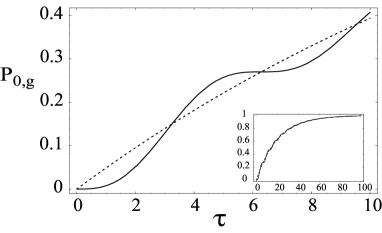
Figure 1: Populations $P_{0,g}(t)$ and $P_{0,g}^{\rm ph}(t)$ vs $\tau=2\Omega t$, when the system starts from the state $\left|0,e\right>$, with $\gamma/2\Omega=0.1$. The solid line refers to the predictions given by the phenomenological master equation, while the dashed line refers to the predictions given by the microscopic one. In the inset it is shown the long time behavior of the same quantities, for $0\leq\tau\leq 100$.

In Fig. 1 we plot the time evolution of the population of the state $\left|0,g\right>$ predicted by both the phenomenological and the microscopic master equations, with $\gamma\left(\omega_{0}-\Omega\right)=\gamma\left(\omega_{0}+\Omega\right)=\gamma=\Omega/5$. This condition legitimates the use of our RWA master equation, while it does not assure the validity of the dressed-state approximation on the phenomenological model, in accordance to geaben . The populations are given by

$$P_{0,g}(t)=\left<0,g\right|\rho(t)\left|0,g\right>=1-\mathrm{e}^{-\frac{\gamma}{2}t},\\$$ (22)

for the predictions of Eq. (21) (microscopic model), as one can see from Eq. (35) in the Appendix putting $\gamma_{a}=\gamma_{b}=\gamma$, and by

$$P_{0,g}^{\rm ph}(t)=\left<0,g\right|\rho(t)\left|0,g\right>=1-\frac{16\Omega^{2}}{16\Omega^{2}-\gamma^{2}}\mathrm{e}^{-\frac{\gamma}{2}t}$$

$$+\frac{\gamma^{2}+\gamma\sqrt{\gamma^{2}-16\Omega^{2}}}{2\left(16\Omega^{2}-\gamma^{2}\right)}\mathrm{e}^{\frac{-\gamma+\sqrt{\gamma^{2}-16\Omega^{2}}}{2}t}$$

$$+\frac{\gamma^{2}-\gamma\sqrt{\gamma^{2}-16\Omega^{2}}}{2\left(16\Omega^{2}-\gamma^{2}\right)}\mathrm{e}^{\frac{-\gamma-\sqrt{\gamma^{2}-16\Omega^{2}}}{2}t},$$ (23)

for the predictions of Eq. (1) (phenomenological master equation).

In both cases, the ground state population of the atom-cavity system increases in time with the same exponential rate, due to the cavity losses. There is, however, an important difference in the behavior predicted by the two equations. Indeed, while our microscopic master equation predicts a purely exponential increase, the phenomenological master equation predicts the presence of oscillations at the Rabi frequency superimposed to the exponential increase. As anticipated, the amplitude of these oscillations is of the order of $\gamma/\Omega$. This difference in the ground state population dynamics reflects different physical mechanisms in the dissipation process. According to the phenomenological master equation, given by Eq. (1), only the cavity can directly lose excitations, as one can see from the form of the dissipator. The rate of loss is indeed proportional to the population of the state $\left|1,g\right>$ only, while the state $\left|0,e\right>$ does not directly decay. In this sense the oscillating behavior of the population of the ground state is a signature of the Rabi oscillations which induce the system decay via the coupling of the state $\left|0,e\right>$ to the state $\left|1,g\right>$.

The microscopic master equation given by Eq. (16), with $\gamma\left(\omega_{0}-\Omega\right)=\gamma\left(\omega_{0}+\Omega\right)$, predicts instead that both the states $\left|1,g\right>$ and $\left|0,e\right>$ decay with the same rate, since they are both superpositions of the states $\left|E_{1,+}\right>$ and $\left|E_{1,-}\right>$. For this reason there is no oscillating behavior in the time evolution of the population of $\left|0,g\right>$.

The difference between the predictions of the phenomenological master equation and those of the microscopic master equation can be revealed by performing joint measurements on both the atom and the cavity, in order to get the population of the state $\left|0,g\right>$ of the composite system.

We can observe a difference in the system dynamics also measuring the population of the atomic ground state, given by $P_{g}(t)=\left<0,g\right|\rho(t)\left|0,g\right>+\left<1,g\right|\rho(t)\left|1,g\right>$. This type of measurement can be performed with standard techniques harocheRMP . With the help of Eq. (21) one finds [See Eqs. (35) and Eq. (36) in the Appendix]

$$P_{g}\left(t\right)=1-\frac{1}{2}\mathrm{e}^{-\frac{\gamma}{2}t}-\frac{1}{4}\left[\mathrm{e}^{\left(2i\Omega-\frac{\gamma}{2}\right)t}-\mathrm{e}^{\left(-2i\Omega-\frac{\gamma}{2}\right)t}\right],$$ (24)

while using Eq. (1) one finds, from Eq.  (23) and Eq. (Appendix) in the Appendix,

$$P_{g}^{\rm ph}(t)=1-\frac{8\Omega^{2}}{16\Omega^{2}-\gamma^{2}}\mathrm{e}^{-\frac{\gamma}{2}t}$$

$$+\frac{2\gamma^{2}+2\gamma\sqrt{\gamma^{2}-16\Omega^{2}}-16\Omega^{2}}{4\left(16\Omega^{2}-\gamma^{2}\right)}\mathrm{e}^{\frac{-\gamma+\sqrt{\gamma^{2}-16\Omega^{2}}}{2}t}$$

$$+\frac{2\gamma^{2}-2\gamma\sqrt{\gamma^{2}-16\Omega^{2}}-16\Omega^{2}}{4\left(16\Omega^{2}-\gamma^{2}\right)}\mathrm{e}^{\frac{-\gamma-\sqrt{\gamma^{2}-16\Omega^{2}}}{2}t}.$$ (25)

In this case, however, the behavior predicted by the phenomenological master equation is very similar to the one predicted by the microscopic one, as one can see from Fig. 2.

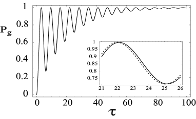
Figure 2: Populations $P_{g}(t)$ and $P_{g}^{\rm ph}(t)$ vs $\tau=2\Omega t$ for the initial state $\left|0,e\right>$, with $\gamma/2\Omega=0.1$. The solid line refers to the predictions given by the phenomenological master equation, while the dashed line refers to the predictions given by the microscopic one. In the large panel, where one can see the long time behavior, the two lines are indistinguishable, while in the inset we have emphasized the dynamics for $21\leq\tau\leq 26$, to put into evidence the presence of the frequency shift.

The only difference, indeed, is the presence of a frequency shift in the Rabi oscillations, as predicted by the phenomenological model. However, since such a shift is of the order of $\left(\gamma/\Omega\right)^{2}$ agar3 , the differences in the predicted behavior may be difficult to detect.

IV.2.2 Decay of a Bell state: exponential vs. oscillatory behavior.

We now consider the case in which the atom-cavity system is initially prepared in a Bell state, such as the state $\left|E_{1+}\right>$, as given by Eq. (II). Contrarily to the case considered in the previous subsection, this time the measurement of the atomic ground state population $P_{g}(t)$ would allow to bring to light the differences in the predictions of the phenomenological and microscopic master equations.

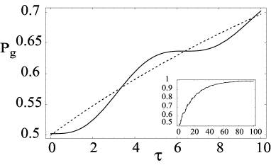
Figure 3: Populations $P_{g}(t)$ and $P_{g}^{\rm ph}(t)$ vs $\tau=2\Omega t$, when the system starts from the state $\left|E_{1,+}\right>$, with $\gamma/2\Omega=0.1$. The solid line refers to the predictions given by the phenomenological master equation, while the dashed line refers to the predictions given by the microscopic one. In the inset one can see the long time behavior of the same quantities for $0\leq\tau\leq 100$.

For the case of the initial state $\left|E_{1+}\right>$ the ground state population is given by

$$P_{g}\left(t\right)=1-\frac{1}{2}\mathrm{e}^{-\frac{\gamma}{2}t},$$ (26)

for the microscopic model [See Eq. (16)] and

$$P_{g}^{\rm ph}(t)=1-\frac{8\Omega^{2}}{16\Omega^{2}-\gamma^{2}}\mathrm{e}^{-\frac{\gamma}{2}t}$$

$$+\frac{\gamma^{2}+\gamma\sqrt{\gamma^{2}-16\Omega^{2}}}{4\left(16\Omega^{2}-\gamma^{2}\right)}\mathrm{e}^{\frac{-\gamma+\sqrt{\gamma^{2}-16\Omega^{2}}}{2}t}$$

$$+\frac{\gamma^{2}-\gamma\sqrt{\gamma^{2}-16\Omega^{2}}}{4\left(16\Omega^{2}-\gamma^{2}\right)}\mathrm{e}^{\frac{-\gamma-\sqrt{\gamma^{2}-16\Omega^{2}}}{2}t},$$ (27)

for the phenomenological model [See Eq. (1)]. Details on the derivation of the above formulas are given in the Appendix.

As we see from Fig. 3, the atomic ground state population, as predicted by the microscopic master equation given by Eq. (16), exhibits a purely exponential behavior while the phenomenological master equation, given by Eq. (1), predicts the presence of oscillations at the Rabi frequency with amplitude of the order of $\gamma/\Omega$. In other words, in the microscopic approach, the atom-cavity system as a whole is subjected to cavity losses and therefore the atom dressed by the cavity mode can directly decay, although it is only the cavity which is directly coupled to the environment.

We stress that, although the generation of a Bell state may be more complicated than the generation of a Fock state, the set of measurements necessary to distinguish between the predictions of the two master equations when the initial state is $\left|E_{1,+}\right>$ is simpler than the set of joint measurements needed in the case of the initial state $\left|0,e\right>$. In fact in the case of the Bell state we just need a way to experimentally distinguish between the atomic excited and ground state, for example by means of a static electric field which ionizes the excited state only, as shown in harocheRMP .

V Discussion and conclusive remarks

In the previous section we have seen that our derivation of the dissipative dynamics of the JC model with losses, taking into account the presence of the atom inside the cavity, allows to give a microscopic description of the interaction between the atom-cavity open quantum system and the external electromagnetic field.

It appears evident from our results that, although the source of the losses is the escape of photons through the cavity mirrors, it is the atom-cavity system as a whole, i.e. the atom dressed by the cavity mode, which comes into play in the dissipative dynamics. Stated another way, while the jump operators appearing in the phenomenological master equations, given by Eq. (1), are the annihilation and creation operators of photons in the cavity ($a$, and $a^{{\dagger}}$), those appearing in the microscopic master equation [See, e.g., Eq. (21)] describe transitions between the dressed states of the atom-cavity system.

A noteworthy point emerging from our analysis is that the deviations of the exactly solved phenomenological model from our microscopic model (coinciding with the one obtained from the phenomenological model with the dressed-state approximation) are of the first order in $\gamma/\Omega$. For this reason it should be possible to check experimentally the predictions of the microscopic model with the set up currently used in cavity QED experiments.

It is worth stressing that in Eq. (1) only one cavity loss rate $\gamma\equiv\gamma(\omega_{0})$, with $\gamma(\omega)$ given by Eq. (10), appears. On the contrary, in Eq. (21), the loss rates corresponding to jump operators connecting the ground state with the states $|E_{1,+}\rangle$ and $|E_{1,-}\rangle$ are different, and more precisely they are given by $\gamma(\omega_{0}+\Omega)$ and $\gamma(\omega_{0}-\Omega)$, respectively. This clearly indicates that, when the spectrum of the reservoir is not flat, the phenomenological master equation does not provide a description which can be justified in terms of a microscopic system-reservoir interaction model as the one we have considered.

In the light of the considerations made above we expect that, already in the weak coupling regime, differences between our approach and the phenomenological one should become evident in those physical contexts where the reservoir is structured, e.g. in photonic band gap materials and hybrid solid-state cavity QED systems photbg1 ; photbg2 ; photbg3 .

Appendix

In this appendix we recall the method of the damping basis introduced in Ref. briegel to solve master equations, and we apply it to Eq. (21).

Given a master equation of the form

$$\dot{\rho}=\mathcal{L}\rho,$$ (28)

where $\mathcal{L}$ is a time-independent linear superoperator acting on $\rho$, one considers the following eigenvalue problem

$$\mathcal{L}\rho_{\lambda}=\lambda\rho_{\lambda},$$ (29)

where $\rho_{\lambda}$ is a right eigenoperator of the superoperator $\mathcal{L}$ with eigenvalue $\lambda$. When the set of right eigenoperators $\left\{\rho_{\lambda}\right\}$ is a basis for the space of linear operators acting on the Hilbert space of the system, as in the case analyzed in this paper, any density operator can be expanded with respect to this set.

It is easy to show that if the system starts from the initial condition

$$\rho(0)=\sum_{\lambda}c_{\lambda}\rho_{\lambda},$$ (30)

then the time evolution of the system is then given by

$$\rho(t)=\sum_{\lambda}c_{\lambda}\mathrm{e}^{\lambda t}\rho_{\lambda}$$ (31)

The coefficients $\left\{c_{\lambda}\right\}$ of the decomposition in Eq. (30) are given by

$$c_{\lambda}=\mathrm{Tr}\left\{\check{\rho}_{\lambda}\,\rho(0)\!\right\},$$ (32)

where $\check{\rho}_{\lambda}$ is the solution of the left eigenvalue problem

$$\check{\rho}_{\lambda}\mathcal{L}=\lambda\check{\rho}_{\lambda},$$ (33)

where the set of left eigenvalues $\left\{\lambda\right\}$ is the same as in the right eigenvalue problem briegel .

When the dimension of the Hilbert space one considers is finite and equal to $n$, the superoperator can be represented by a non-hermitian $n^{2}\times n^{2}$ matrix. The right eigenoperators, if they exist, are represented by $n^{2}$-component column vectors, while the left eigenoperators are represented by $n^{2}$-component row vectors.

Applying this method to Eq. (21), we have to look for the nine right eigenoperators of its superoperator. For simplicity we call $\gamma_{a}=\gamma\left(\omega_{0}-\Omega\right)$ and $\gamma_{b}=\gamma\left(\omega_{0}+\Omega\right)$.

Six of the nine right eigenoperators are given by the coherences $\left|E_{0}\right>\left<E_{1,-}\right|$, $\left|E_{0}\right>\left<E_{1,+}\right|$, $\left|E_{1,-}\right>\left<E_{1,+}\right|$ and their hermitian conjugates, with eigenvalues respectively equal to $i\left(\omega_{0}-\Omega\right)-\gamma_{a}/2$, $i\left(\omega_{0}+\Omega\right)-\gamma_{b}/2$, $i(2\Omega)-\left(\gamma_{a}+\gamma_{b}\right)/4$ and their complex conjugates. The other three right eigenoperators are given by $\left|E_{0}\right>\left<E_{0}\right|$, $\left(\left|E_{1,-}\right>\left<E_{1,-}\right|-\left|E_{0}\right>\left<E_{0}\right|\right)$, $\left(\left|E_{1,+}\right>\left<E_{1,+}\right|-\left|E_{0}\right>\left<E_{0}\right|\right)$ with eigenvalues respectively equal to $0$, $-\gamma_{a}/2$ and $-\gamma_{b}/2$.

By expanding the initial state with respect to these nine eigenoperators, one can then compute the evolution of the system under the initial conditions given in part B of Sec. IV.

When the initial state is $\rho(0)=\left|0,e\right>\left<0,e\right|$ one obtains the following density operator at time $t$

$$\rho(t)=\left(1-\frac{1}{2}\mathrm{e}^{-\frac{\gamma_{a}}{2}t}-\frac{1}{2}\mathrm{e}^{-\frac{\gamma_{b}}{2}t}\right)\left|E_{0}\right>\left<E_{0}\right|$$

$$+\frac{1}{2}\mathrm{e}^{-\frac{\gamma_{a}}{2}t}\left|E_{1,-}\right>\left<E_{1,-}\right|+\frac{1}{2}\mathrm{e}^{-\frac{\gamma_{b}}{2}t}\left|E_{1,+}\right>\left<E_{1,+}\right|$$

$$-\frac{1}{2}\mathrm{e}^{-\frac{\gamma_{a}+\gamma_{b}}{4}t}\left(\mathrm{e}^{2i\Omega t}\left|E_{1,-}\right>\left<E_{1,+}\right|+\mbox{h.c.}\right),$$ (34)

which allows us to express the population of the state $\left|0,g\right>$ as follows

$$P_{0,g}(t)=\left<0,g\right|\rho(t)\left|0,g\right>=1-\frac{1}{2}\mathrm{e}^{-\frac{\gamma_{a}}{2}t}-\frac{1}{2}\mathrm{e}^{-\frac{\gamma_{b}}{2}t}.\\$$ (35)

The population of the state $\left|1,g\right>$ is given by

$$P_{1,g}(t)=\left<1,g\right|\rho(t)\left|1,g\right>=\frac{1}{4}\left[\mathrm{e}^{-\frac{\gamma_{a}}{2}t}+\mathrm{e}^{-\frac{\gamma_{b}}{2}t}\right.$$ (36)

$$\left.-\mathrm{e}^{\left(2i\Omega-\frac{\gamma_{a}+\gamma_{b}}{4}\right)t}-\mathrm{e}^{\left(-2i\Omega-\frac{\gamma_{a}+\gamma_{b}}{4}\right)t}\right].$$

Using the two equations above one can calculate $P_{g}(t)=\left<g\right|\rho(t)\left|g\right>=\left<0,g\right|\rho(t)\left|0,g\right>+\left<1,g\right|\rho(t)\left|1,g\right>$ given in Eq. (24).

Equation (35) and Eq. (36) are to be compared with the corresponding quantities computed using the phenomenological master equation, given by Eq. (1), and considering the same initial condition. Following the same lines one derives Eq. (23) for the population of the ground state $\left|0,g\right>$ and

$$P_{1,g}^{\rm ph}(t)=\left<1,g\right|\rho(t)\left|1,g\right>=\frac{8\Omega^{2}}{16\Omega^{2}-\gamma^{2}}\mathrm{e}^{-\frac{\gamma}{2}t}$$

$$-\frac{16\Omega^{2}}{4\left(16\Omega^{2}-\gamma^{2}\right)}\mathrm{e}^{\frac{-\gamma+\sqrt{\gamma^{2}-16\Omega^{2}}}{2}t}$$

$$-\frac{16\Omega^{2}}{4\left(16\Omega^{2}-\gamma^{2}\right)}\mathrm{e}^{\frac{-\gamma-\sqrt{\gamma^{2}-16\Omega^{2}}}{2}t},$$ (37)

for the population of state $\left|1,g\right>$.

In the same way one can derive the time evolution predicted by the microscopic master equation (21) when the initial condition is $\rho(0)=\left|E_{1,+}\right>\left<E_{1,+}\right|$:

$$\rho(t) =\left(1-\mathrm{e}^{-\frac{\gamma_{b}}{2}t}\right)\left|E_{0}\right>\left<E_{0}\right|$$ (38)

$$+\mathrm{e}^{-\frac{\gamma_{b}}{2}t}\left|E_{1,+}\right>\left<E_{1,+}\right|,$$

which gives the following expressions for the populations of states $\left|0,g\right>$ and $\left|1,g\right>$

$$P_{0,g}(t)=\left<0,g\right|\rho(t)\left|0,g\right>=1-\mathrm{e}^{-\frac{\gamma_{b}}{2}t},$$

$$P_{1,g}(t)=\left<1,g\right|\rho(t)\left|1,g\right>=\frac{1}{2}\mathrm{e}^{-\frac{\gamma_{b}}{2}t}.$$ (39)

Once more, we must compare these expressions with the corresponding ones obtained by means of the phenomenological master equation given by Eq. (1). Using this equation one obtains

$$P_{0,g}^{\rm ph}(t)=\left<0,g\right|\rho(t)\left|0,g\right>=1-\frac{16\Omega^{2}}{16\Omega^{2}-\gamma^{2}}\mathrm{e}^{-\frac{\gamma}{2}t}$$

$$+\frac{\gamma^{2}}{2\left(16\Omega^{2}-\gamma^{2}\right)}\mathrm{e}^{\frac{-\gamma+\sqrt{\gamma^{2}-16\Omega^{2}}}{2}t}$$

$$+\frac{\gamma^{2}}{2\left(16\Omega^{2}-\gamma^{2}\right)}\mathrm{e}^{\frac{-\gamma-\sqrt{\gamma^{2}-16\Omega^{2}}}{2}t},$$ (40)

for the population of $\left|0,g\right>$, and

$$P_{1,g}^{\rm ph}(t)=\left<1,g\right|\rho(t)\left|1,g\right>=\frac{8\Omega^{2}}{16\Omega^{2}-\gamma^{2}}\mathrm{e}^{-\frac{\gamma}{2}t}$$

$$-\frac{\gamma^{2}-\gamma\sqrt{\gamma^{2}-16\Omega^{2}}}{4\left(16\Omega^{2}-\gamma^{2}\right)}\mathrm{e}^{\frac{-\gamma+\sqrt{\gamma^{2}-16\Omega^{2}}}{2}t}$$

$$-\frac{\gamma^{2}+\gamma\sqrt{\gamma^{2}-16\Omega^{2}}2}{4\left(16\Omega^{2}-\gamma^{2}\right)}\mathrm{e}^{\frac{-\gamma-\sqrt{\gamma^{2}-16\Omega^{2}}}{2}t},$$ (41)

for the population of $\left|1,g\right>$.

References

- (1) E.T. Jaynes and F.W. Cummings, Proc. IEEE 51, 89 (1963).
- (2) For a review see B.W. Shore and P.L. Knight, J. Mod. Opt. 40, 1195 (1993).
- (3) R.R. Puri, Mathematical Methods of Quantum Optics (Springer, 2001).
- (4) S. Haroche et al., in Fundamental Systems in Quantum Optics, ed. by J. Dalibard, J.-M. Raimond and J. Zinn-Justin (North Holland, 1992).
- (5) J.M. Raimond et al., Rev. Mod. Phys. 73, 565 (2001).
- (6) H. Walther et al., Rep. Prog. Phys. 69, 1325 (2006).
- (7) D. Wineland et al., J. Res. Natl. Inst. Stand. Technol. 103, 258 (1998).
- (8) J. Gea-Banacloche, Phys. Rev. A 47, 2221 (1993).
- (9) C. Cohen-Tannoudji et al., Atom-Photon Interactions (John Wiley, New York, 1998).
- (10) G.S. Agarwal and R.R. Puri, Phys. Rev. A 33, 1757 (1986).
- (11) R.R. Puri and G.S. Agarwal, Phys. Rev. A 33, 3610 (1986).
- (12) R.R. Puri and G.S. Agarwal, Phys. Rev. A 35, 3433 (1987).
- (13) S.M. Barnett and P.L. Knight, Phys. Rev. A 33, 2444 (1986).
- (14) H.-J. Briegel and B.-G. Englert, Phys. Rev. A 47, 3311 (1993).
- (15) H.-P. Breuer and F. Petruccione, The Theory of Open Quantum systems (Oxford University Press, 2002).
- (16) H. Spohn and J.L. Lebowitz, Adv. Chem. Phys. 38, 109 (1979).
- (17) T. Quang and S. John, Phys. Rev. A 56, 4273 (1997).
- (18) L. Florescu, S. John, T. Quang, and R. Wang, Phys. Rev. A 69, 013816 (2006).
- (19) B. Lev et al., Nanotechnology 15, S556 (2004)