Regular and Chaotic Quantum Dynamic in Atom-Diatom Reactive Collisions

Abstract

A new micro-irreversible $3D$ theory of quantum multichannel scattering in the three-body system is developed. The quantum approach is constructed on the generating trajectory tubes which allow taking into account influence of classical non-integrability of the dynamical quantum system. When the volume of classical chaos in phase space is larger than the quantum cell in the corresponding quantum system, quantum chaos is generated. The probability of quantum transitions is constructed for this case. The collinear collision of the $Li+(FH)\to(LiF)+H$ system is used for numerical illustration of a system generating quantum (wave) chaos.

I Introduction

In the early stage of quantum mechanics development A. Einstein asked a question that have attracted close attention several decades later Ein . The question was: what would be the analogue of a classical chaotic system in quantum mechanics? In particular he pointed to the three-body system, which in general is well known to have a chaotic nature.

In an effort to formulate and obtain the solution of the problem of quantum chaos, M. Gutzwiller tentatively divided all the existing knowledge of the dynamics of physical systems into three areas Gutz :

1. Regular classical mechanics ($R$ area);

2. Classical chaotic system or dynamical Poincare system ($P$ area);

3. Regular quantum mechanics ($Q$ area).

The mentioned areas are connected by certain conditions. Thus, Bohr’s correspondence principle connects the $R$ and $Q$ areas, transferring quantum mechanics into classical Newtonian mechanics in the limit $\hbar\rightarrow 0$. Areas $R$ and $P$ are connected by the Kolmogorov-Arnold-Moser (KAM) theorem.

The general principle which can connect $P$ and $Q$ areas is not determined yet. Related to the fourth, conditionally named the quantum chaos area $Q_{ch}$, M.  Gutzwiller mentioned that the ”quantum chaos” conception is rather a puzzle than a well formulated problem. It is evident that the task formulated correctly in $Q_{ch}$ area is the most general one and under specific conditions must be transformed into the aforementioned limiting areas.

Observation of chaotic phenomena in the spectroscopy of atomic nuclei Brody , atoms Fried , molecules Nemes and in billiard systems Miln -Dembr has stimulated a considerable interest in the quantum chaos problem in recent years. Irregular behavior of the wavefunction has been found in numerical calculations of quantum mechanical stadium billiard problem McDonald . It has been shown that the so called scars which were observed have classical trajectory characteristics Heller . It has been known for a long time that classical models of chemical reactions exhibit chaos Hamilton . It was shown that the mixing properties of chaotic dynamics observed in unimolecular reactions can be explained by some statistical laws Marcus . Recall that one major motivation for the continued classical investigation of the reactive scattering problem Kovacs -Ott is several kinds of experiments on waves, which have demonstrated the validity of the ideas of quantum chaotic scattering Smilansky -Dorn . Atomic systems are quantum objects should thus be treated considering their quantum properties.

The development of different semiclassical and mixed quantum-classical methods (see for example the detailed report Nyman ) can be considered as a natural extension of the classical trajectory study. This development has been motivated by the fact that the standard quantum approach is too demanding even for most few-body systems. For many problems various quasi-classical methods can give satisfactory results. The semiclassical methods, however, are restricted to relatively small systems.

The problem of quantum chaos and its connection with classical nonintegrability was originally studied by the authors in the framework of a collinear three-body collision model Gev . In the current article this approach is generalized to the $3D$ case.

II Formulation of scattering problem

We will be interested in the three-body reactive scattering process $A+(BC)_{n}\to(ABC)^{*}\to(AB)_{m}+C$, where $A,B,$ and $C$ are atoms, $n$ and $m$ characterize the set of quantum numbers of diatomic states corresponding to initial $(in)$ and final $(out)$ scattering arrangements and $(ABC)^{*}$ denotes the resonance complex. Moreover $m_{A},m_{B}$ and $m_{C}$ are the masses of the particles and ${\bf{r_{A}}},{\bf{r_{B}}}$ and ${\bf{r_{C}}}$ the column vectors describing their positions relative to an origin fixed in the laboratory system. The reactant arrangement is best described by mass scaled reactant Jacobi co-ordinates, while the product arrangement is best described by mass scaled product Jacobi coordinates. For the reactant arrangement we can write Delves ; Smith :

$${\bf{q}_{0\alpha}}=\lambda\,{\bf{R}}_{\alpha},\qquad{\bf{q}_{1\alpha}}=\lambda^{-1}\,{\bf{r}}_{\alpha},$$ (1)

where $\bf{R}_{\alpha}$ and ${\bf{r}}_{\alpha}$ Jacobi coordinates of reactant $(in)$ channel, moreover: $\lambda=\bigl{[}m_{A}\bigl{(}1-m_{A}/{M}\bigr{)}/\mu\bigr{]}^{1/2},\quad\mu=\bigl{[}m_{A}m_{B}m_{C}/M\bigr{]}^{1/2},\quad M=m_{A}+m_{B}+m_{C}.$ In term of coordinates $({\bf{q}_{0\alpha}},{\bf{q}_{1\alpha}})$ the Hamiltonian of three-body system takes:

$$H\bigl{(}{\bf{q}};{\bf{P_{{\bf{q}}}}}\bigr{)}=\bigl{(}1/2\mu\bigr{)}{\bf{P}}_{\bf{q}}^{2}+V\bigl{(}q_{0},q_{1},\theta\bigr{)},\qquad\bf{q}=\bigl{(}{\bf{q}_{0}},{\bf{q}_{1}})=\{q_{k}\},\quad k=0,...,5.$$ (2)

Note that here and in the following we omit the channel index for simplicity. In (2) $\mu$ and ${\bf{P}_{\bf{q}}}$ are the effective mass and moment of body system, $(q_{0}=|{\bf{\bf{q_{0}}}}|,q_{1}=|{\bf{\bf{q_{1}}}}|,\theta)$ characterizes the intrinsic coordinates, $\theta$ is the angle between vectors ${\bf{\bf{q_{0}}}}$ and ${{\bf{q_{1}}}}$. The remaining coordinates $(q_{3},q_{4},q_{5})$ are expresses via Euler angles. The interaction potential between all atoms $V\bigl{(}q_{0},q_{1},\theta\bigr{)}$ depends on intrinsic coordinates.

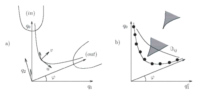
Figure 1: a) Intrinsic Jacobi and local coordinate systems. The angle $\vartheta$ is defined from $\cot\vartheta=b=\sqrt{{m_{A}m_{C}}\bigl{/}{m_{B}M}}$. b) The reaction path is passing through the minimums of potential energy while the reaction coordinate $\Im_{if}$ can be an arbitrary smooth curve connecting $(in)$ and $(out)$ asymptotic channels. The lower shaded area is self-crossing region for natural collision coordinate (NCC) system associated to the reaction path curve while the upper one self-crossing region for NCC system is associated to the curve $\Im_{if}$.

Recall, that the coordinate systems needed for reactants and products are different Nyman . This fact creates certain mathematical and computational complexities for the investigation of multichannel scattering problem. The way to overcome it is to turn to special type of curvilinear coordinates, which are natural and suitable for description of two (or more) asymptotical states $(in)$ and $(out)$ simultaneously. For satisfying of this conditions in the collinear collision case was introduced smooth curve $\Im_{if}$ (coordinate reaction) which connected $(in)$ and $(out)$ asymptotical channels and along which was defined local orthogonal coordinates system $(u,v)$ (see Marcus1 ; Light ).

In 3$D$ case too we can introduce the curve $\Im_{if}$, along which NCC system is defined. In this case $\Im_{if}$ is defined on the plane $(q_{0},q_{1},\theta=0)$ by expression Gev4 :

$$q_{0}^{c}=a\bigl{/}\bigl{(}{q_{1}^{c}-q_{eq}^{-}}\bigr{)}+bq_{1}^{c}+q^{+}_{eq},\qquad\qquad\qquad q_{eq}^{-}<q_{1}^{c}<\infty,$$ (3)

where $a$ and $b$ are constants. In Eq. (3) $q^{-}_{eq}$ and $q^{+}_{eq}$ are mass-scaled equilibrium bond lengths of molecules in the $(in)$ and $(out)$ channels respectively, $a$ is an arbitrary constant, which is usually chosen to make the curve pass close to the saddle point of the reaction. The superscript $c$ over $q_{0}$ and $q_{1}$ underlines the fact that the point $(q_{0}^{c},q_{1}^{c})$ lies on the curve. The limit $(q_{1}=0,\,\,q_{0}\rightarrow{\infty})$ corresponds to the $(in)$ state, while the limit $(q_{0}=bq_{1}=q_{1}\cot\vartheta)$ corresponds to the $(out)$ state. The movement along the curve $\Im_{if}$ is described by the coordinate $u$:

$$u=u_{0}-a\bigl{/}\bar{q}_{1}^{c}+b\bar{q}_{1}^{c},\qquad\bar{q}_{1}^{c}=q_{1}^{c}-q_{eq}^{-},$$ (4)

where $u_{0}$ is some initial point on the curve $\Im_{if}$. The inverse transformations between the two pairs of coordinates $(q_{0},q_{1})\Leftrightarrow(u,v)$ are:

$$q_{0}(u,v)=q_{0}^{c}(u)-v\sin\phi(u),\quad q_{1}(u,v)=q_{1}^{c}(u)+v\cos\phi(u),$$ (5)

where $v$ is the distance from the curve $\Im_{if}$. In Eq. (5) the angle $\phi(u)$ is determined by requiring orthogonality of coordinate system $(u,v)$:

$${dq_{0}^{c}}/{dq_{1}^{c}}\Bigl{|}_{(u,v=0)}=\cot\phi(u),\qquad\lim_{u\rightarrow+\infty}\cot\phi(u)=\cot\vartheta.$$ (6)

Let us introduce the system of orthogonal local coordinates ${\bf{x}}\equiv{\bf{x}}(x^{0},x^{1},...x^{5})$ along the curve $\Im_{if}$ using the transformations:

$$x^{0}=u,\quad x^{1}=v,\quad\,x^{2}=f(u,v,\theta),\quad x^{3}=d_{0}\omega_{1},\quad x^{4}=d_{0}\omega_{2},\quad x^{5}=d_{0}\omega_{3},$$ (7)

where function $f(u,v,\theta)=\sqrt{(q_{0})^{2}-2bq_{0}q_{1}\cos\theta+b^{2}(q_{1})^{2}}$ is mass-scale distance between $A$ and $B$ particles. In some part of the $3D$ Cartesian configuration space these equations determine a biunivocal mapping between the two intrinsic coordinate systems: $\{q_{0},q_{1},\theta\}$ and $\{x^{0},x^{1},x^{2}\}$. The set of coordinates $(\omega_{1},\omega_{2},\omega_{3})$ are three Euler angles, which orient the three-body system in the space-fixed frame Balint1 , $d_{0}$ is some space-dimensional constant.

II.1 Classical dynamics of three-body scattering system

For the investigation of ergodic properties of conservative dynamical system the geodesic axes distribution method on Riemann surfaces had been originally applied in Hoft . Later this method has been used and developed in the investigations of the foundations of statistical physics Krylov . The study of geodesic flow behavior on Lagrange surfaces provides an opportunity to observe important properties of classical dynamics systems katok .

Consider the $6D$ three-body classical problem on the Lagrange surface $S_{P}$:

$$S_{P}=\bigl{\{}{\bf{x}};\,P^{2}(u,v,\theta)=2\mu\bigl{[}E-U(u,v,\theta)\bigr{]}>0\bigr{\}},$$ (8)

where $E$ is the total energy and $U(u,v,\theta)$ is the interaction potential of the three-body system. The metric on the surface $S_{P}$ is introduced in conform-Euclidian form:

$$(ds)^{2}=\sum_{i,j}g_{ij}dx^{i}dx^{j},\qquad g_{ij}(u,v,\theta)=P^{2}(u,v,\theta)\delta_{ij},\quad i,j=0,1,...,5.$$ (9)

Now we can write the geodesic trajectory problem for the reduced mass $\mu$:

$$x^{k}_{;ss}+\Gamma^{k}_{ij}x^{i}_{;s}x^{j}_{;s}=0,\qquad i,j,k=0,1,...,5,$$ (10)

where $s$ is a natural parameter (time or length of the geodesic trajectory), $\Gamma^{k}_{ij}=\frac{1}{2}g^{kl}\Bigl{(}\frac{\partial g_{lj}}{\partial x^{i}}+\frac{\partial g_{il}}{\partial x^{j}}-\frac{\partial g_{ij}}{\partial x^{l}}\Bigr{)}$ is a Cristoffel symbol. Moreover $x^{i}_{;s}=\frac{dx^{i}}{ds}$ and $x^{i}_{;ss}=\frac{d^{2}x^{i}}{ds^{2}}.$

The system of differential equations (10) is solved for the initial conditions:

$$x^{i}_{0}=x^{i}(-\infty),\qquad\dot{x}^{i}_{0}=x^{i}_{;s}(-\infty),$$ (11)

for any value of the natural parameter $s$ from which the geodesic trajectory $x^{i}(s)$ and the geodesic velocity $x^{i}_{;s}(s)$ are defined. Using the relations in Eqs. (9) and (10) it is not complicated to obtain the following system of equations:

$$x^{0}_{;ss}+\frac{1}{2}\frac{\partial{\chi}}{\partial{x^{0}}}\biggl{\{}\bigl{(}x_{;s}^{0}\bigr{)}^{2}-\bigl{(}x_{;s}^{1}\bigr{)}^{2}-\bigl{(}x_{;s}^{2}\bigr{)}^{2}-\frac{I^{2}}{\mu^{2}g_{00}^{2}}\biggr{\}}+\biggl{\{}\frac{\partial{\chi}}{\partial{x^{1}}}x^{1}_{;s}+\frac{\partial{\chi}}{\partial{x^{2}}}x^{2}_{;s}\biggr{\}}x_{;s}^{0}=0,\quad$$

$$x^{1}_{;ss}+\frac{1}{2}\frac{\partial{\chi}}{\partial{x^{1}}}\biggl{\{}\bigl{(}x_{;s}^{1}\bigr{)}^{2}-\bigl{(}x_{;s}^{0}\bigr{)}^{2}-\bigl{(}x_{;s}^{2}\bigr{)}^{2}-\frac{I^{2}}{\mu^{2}g_{00}^{2}}\biggr{\}}+\biggl{\{}\frac{\partial{\chi}}{\partial{x^{0}}}x^{0}_{;s}+\frac{\partial{\chi}}{\partial{x^{2}}}x^{2}_{;s}\biggr{\}}x_{;s}^{1}=0,\quad$$

$$x^{2}_{;ss}+\frac{1}{2}\frac{\partial{\chi}}{\partial{x^{2}}}\biggl{\{}\bigl{(}x_{;s}^{2}\bigr{)}^{2}-\bigl{(}x_{;s}^{0}\bigr{)}^{2}-\bigl{(}x_{;s}^{1}\bigr{)}^{2}-\frac{I^{2}}{\mu^{2}g_{00}^{2}}\biggr{\}}+\biggl{\{}\frac{\partial{\chi}}{\partial{x^{0}}}x^{0}_{;s}+\frac{\partial{\chi}}{\partial{x^{1}}}x^{1}_{;s}\biggr{\}}x_{;s}^{2}=0,\quad$$ (12)

where $\chi(x^{0},x^{1},x^{2})=\ln g_{00}(x^{0},x^{1},x^{2})$, the $I$ is total angular momentum of three-body system. It is suitable to conduct the later calculation in the $(u,v,\theta)$ coordinates system. Because the explicit form of equation system in those coordinates is complicated, we don’t write down them here.

We have now formulated the reactive scattering problem in terms of classical dynamics on the Lagrange surface of the three-body system. Note, that the system has one integral of motion (overall energy $E$) and three degrees of freedom.

According to Poincare (see katok ), conservative dynamical systems can have regions of chaotic movement in their phase space provided that they are not integrable, i.e. have less integrals of motion than degrees of freedom. This means that certain areas in phase space may show non-stability and chaos may then be observed, i.e. the trajectory $x^{j}(s)$ then becomes exponentially non-stable with respect to change of the initial condition $x^{j}(0)$:

$${\partial{x^{j}(s)}}/{\partial{x^{j}(0)}}\sim\exp(\lambda_{j}{s}),\quad j=0,1,2,$$ (13)

where $\lambda_{j}$ describes the degree of instability and is called Lyapunov exponent.

II.2 Quantization of classical dynamical three-body scattering system

Representation for regular case:

In some coordinate systems, like the NCC system, Gev4 the $3D$ quantum reactive scattering problem can be treated in the same way as an inelastic single-arrangement problem. The overall wavefunction of the three body system can be represented:

$${\Phi}^{(+)J}_{K^{\prime}\varrho}(u,v,\theta)=\sum_{\bar{n}\bar{j}}{G}^{(+)J}_{\bar{n}\bar{j}K^{\prime}\,\varrho}(u)\Xi_{\bar{n}(\bar{j})}(v;u)\Theta_{\bar{j}K^{\prime}}(\theta),\quad\varrho=(njK),$$ (14)

where $(n,j,K)$ is a set of quantum numbers, $\Theta_{jK}(\theta)$ is a normalized associated Legendre polynomial, $\Xi_{n(j)}(v;u)$ is the vibrational part of the wavefunction and satisfies the equation:

$$\biggl{[}-\frac{\,\hbar^{2}}{2\mu}\frac{d^{\,2}}{dv^{2}}+\overline{U}(u,v)+\frac{\hbar^{2}j(j+1)}{2\mu{v^{2}}}\biggr{]}\Xi_{n(j)}(v;u)=\epsilon_{n(j)}(u)\,\Xi_{n(j)}(v;u),$$ (15)

where $\overline{U}(u,v)=U(u,v,\theta)\bigl{|}_{\theta=0}-U_{eff}(u,v)$. The function $U(u,v,\theta)\bigl{|}_{\theta=0}$ describes the potential energy of the collinear collision. $U_{eff}(u,v)$ is an effective potential:

$$U_{eff}(u,v)=\frac{1}{4\eta^{2}}\biggl{(}\frac{\partial\eta}{\partial{v}}\biggr{)}^{2}-\frac{1}{2\eta^{3}}\frac{\partial^{2}\eta}{\partial{u^{2}}}+\frac{5}{4\eta^{4}}\biggl{(}\frac{\partial\eta}{\partial{u}}\biggr{)}^{2},\quad\eta(u,v)=\bigl{[}1+K(u)v\bigr{]}\frac{ds}{du}.\quad$$ (16)

In eqn. (16), $K(u)$ is the curvature of $u$ and $s$ is the length along the curve $\Im_{ij}$:

$$K(u)=2a\frac{\bigl{[}F(q_{1}^{c})\bigr{]}^{-3/2}}{\bigl{(}q_{1}^{c}-q_{eq}^{-}\bigr{)}^{3}},\quad\frac{ds}{du}=\frac{\sqrt{F(q_{1}^{c})}}{b+a/{\bigl{(}q_{1}^{c}-q_{eq}^{-}\bigr{)}^{2}}},\quad F(q_{1}^{c})=1+\Bigl{[}b-a/{\bigl{(}q_{1}^{c}-q_{eq}^{-}\bigr{)}^{2}}\Bigr{]}^{2}.$$ (17)

Note, that the scattering function ${G}^{(+)J}_{\bar{n}\bar{j}K^{\prime}\varrho}(u)$ satisfies the following equation:

$$\Biggl{\{}\biggl{[}\delta_{n^{\prime}\bar{n}}\frac{d^{2}}{d{u^{2}}}+2\biggl{<}\frac{\partial}{\partial{u}}-\frac{1}{\eta}\frac{\partial\eta}{\partial{u}}\biggr{>}_{n^{\prime}\bar{n}}\frac{d}{d{u}}+\biggl{<}\frac{\partial^{2}}{\partial{u^{2}}}-\frac{2}{\eta}\frac{\partial\eta}{\partial{u}}\frac{\partial}{\partial{u}}\biggr{>}_{n^{\prime}\bar{n}}+\frac{2\mu}{\hbar^{2}}\biggl{<}\eta^{2}\Bigl{[}E-E_{J\bar{K}}\quad$$

$$-\epsilon_{\bar{n}(\bar{j}\,)}(u)+U(u,v)+\frac{\hbar^{2}\bar{j\,}(\bar{j\,}+1)}{2\mu{v^{2}}}\Bigr{]}\,\biggl{>}_{n^{\prime}\bar{n}}\,\,\biggr{]}\delta_{j\,^{\prime}\bar{j\,}}\delta_{K^{\prime}\bar{K}}-\frac{2\mu}{\hbar^{2}}\Bigl{<}\eta^{2}\,U_{j\,^{\prime}\bar{j\,}}^{\bar{K}}(u,v)\Bigr{>}_{n^{\prime}\bar{n}}\,\delta_{K^{\prime}\bar{K}}\quad$$

$$+\Bigl{<}\,\frac{\eta^{2}}{q_{0}^{2}}\,\Bigr{>}_{n^{\prime}\bar{n}}\,\delta_{j\,^{\prime}\bar{j\,}}\left[\delta_{K^{\prime}+1\,\bar{K}}\,{C_{J\bar{j\,}(\bar{K}-1)}^{+}+\delta_{K^{\prime}-1\,\bar{K}}\,C_{J\bar{j\,}(\bar{K}+1)}^{-}}\right]\Biggr{\}}{G}^{(+)J}_{\bar{n}\bar{j\,}\bar{K}\,\varrho}(u)=0,\qquad\quad$$ (18)

where $C^{\pm}_{JjK}=c^{\pm}_{JK}c^{\pm}_{jK}$, and moreover:$c^{\pm}_{JK}=\bigl{[}J(J+1)-K(K\pm 1)\bigr{]}^{1/2},\quad E_{JK}(u,v)=(1/2){\hbar^{2}}{\mu}^{-1}q_{0}^{-2}(u,v)\bigl{(}J(J+1)-2K^{2}\bigr{)}.$ The summations over the repeating index $n^{\prime}$ and $j\,^{\prime}$ are implied and we use the following notations for the matrix elements:

$$\bigl{<}f(u)\bigr{>}_{nn^{\prime}}=\int^{+\infty}_{-\infty}\Xi_{n(j)}(v;u)f(u,v)\Xi_{n^{\prime}(j)}^{\ast}(v;u)dv,$$

$$U^{K}_{jj\,^{\prime}}(u,v)=\int^{\pi}_{0}{\Theta_{jK}(\theta)\,U(u,v,\theta)\,\Theta_{j^{\prime}K}(\theta)}\sin\theta{d\theta}.$$ (19)

Note, that the solution of Eq. (18) is must satisfy the asymptotic condition:

$$\lim_{u\rightarrow-\infty}\sum_{n^{\prime}j\,^{\prime}}{G}^{(+)J}_{n^{\prime}j\,^{\prime}K^{\prime}\,\varrho}(u)=\frac{1}{\sqrt{2\pi}}\exp\left(-ip_{nj}^{-}\,u\right)\delta_{nn^{\prime}}\delta_{jj\,^{\prime}}\delta_{KK^{\prime}}.$$ (20)

The exact S-matrix elements can be constructed in terms of stationary overall and asymptotic wavefunctions, considering that the variable $u$ plays the role of a timing parameter ( which later will be called internal time) Gev4 :

$$\emph{S}_{n^{\prime}j\,^{\prime}K^{\prime}\,\leftarrow\,njK}(E)=\sqrt{{p^{+}_{n^{\prime}j\,^{\prime}}}\bigl{/}{p^{-}_{nj}}}\,\lim_{u\rightarrow+\infty}\sum_{\bar{n}\bar{j}}G^{(+)J}_{\bar{n}\bar{j}K^{\prime}\,\varrho}(u)\,W_{\bar{n}n^{\prime}}(u)\Lambda_{\bar{j}K^{\prime}\,\leftarrow\,jK^{\prime}},$$ (21)

where $W_{n^{\prime}\bar{n}}(u)=\bigl{\langle}\Xi_{\bar{n}(\bar{j\,})}(v;u)\Pi_{n^{\prime}(j\,^{\prime})}^{(out)}(v)\bigr{\rangle}_{v},\quad\Lambda_{\bar{j}K^{\prime}\,\leftarrow\,jK^{\prime}}=\bigl{<}\Theta_{\bar{j\,}K^{\prime}}(\theta)\Theta_{jK^{\prime}}(\theta)\bigr{>}_{\theta}=\delta_{\bar{j\,}j}.$ The expression for the S-matrix elements in eqn. (21) can be simplified, if we take as basis the functions $\Xi_{n(j)}(v;u)$, which in the limit $u\rightarrow+\infty$ coincide with the orthonormal basis of the $(out)$ asymptotic wavefunctions $\Pi_{n(j)}^{(out)}(v)$. In this case we get the simplification $\lim_{u\rightarrow+\infty}W_{n^{\prime}\bar{n}}(u)=\delta_{n^{\prime}\bar{n}}$ and the following expression holds for the S-matrix elements:

$$\emph{S}_{n^{\prime}j\,^{\prime}K^{\prime}\,\leftarrow\,njK}(E)=\sqrt{{p^{+}_{n^{\prime}j\,^{\prime}\,}}\bigl{/}{p^{-}_{nj}}}\,{G}^{(+)J}_{\varrho\,^{\prime}\varrho}(E;+\infty),\qquad\varrho=(njK).$$ (22)

Representation for chaotic case: It is well known that some chemical reactions, especially when highly excited, exhibit quantum chaotic behavior Gutz ; Honv , i.e., the statistical properties of eigen-energies and eigen-vectors are very similar to those of random matrix systems Hak ; Mehta .

For systems which are not too quantum mechanical in nature, the quantum probability current is localized along the classical trajectory. In the chaotic case, these classical trajectories diverge exponentially from each other and from the quantum current tubes too. This results in serious difficulties in describing chaotic reactive quantum processes in terms of standard quantum representations. In order to overcome the this problem, a new quantization method bases on the quasi-classical approach has been proposed Gev for the three-body system. The idea is to carry out the quantization on separate classical trajectory tubes $\Re({\bf{x}}_{3}(s))$, where ${\bf{x}}_{3}(s)\equiv{\bf{x}}_{3}\bigl{(}u(s),v,\theta\bigr{)}$ and $u(s)$ is the solution of the geodesic equations (12), which varies along the curve $\Im_{if}$ and is called as a generating trajectory (recall that it has the meaning of internal time). Every solution $u(s)$ generates some topological trajectory tube, which can be described by the Schrödinger equation, which for the present case means Eq. (18). The summed contribution of all such tubes gives the whole quantum picture.

The goal of the scattering problem is the calculation of the probability amplitudes for transitions between different asymptotic states. In mathematical language this corresponds to the determination of the total mathematical expectation of the elementary quantum process in the three-body system. In the classical case the solution $u(s)$ depends on the initial scattering phase $\varphi=2\pi\{u/L\}$, as does then the overall wavefunction and $S$-matrix elements. Here $L$ is a some period and $\{\cdot\}$ describes a fractional part of the function. This implies that the transition amplitude $\bigtriangleup_{\varrho\,^{\prime}\,\varrho}=\bigl{|}\emph{S}_{\varrho\,^{\prime}\,\leftarrow\,\varrho}(\varphi;E)\bigl{|}^{2}$ must be averaged over the $\varphi$ phase distribution:

$$W_{\varrho\,^{\prime}\,\leftarrow\,\varrho}(E)=\frac{\int\sigma(\varphi;E)\bigtriangleup_{\varrho\,^{\prime}\,\,\varrho}(\varphi\,;E)\,d\varphi}{\int\sigma(\varphi;E)d\varphi},$$ (23)

where $\sigma(\varphi;E)$ is the distribution of classical trajectories which will be determined later in the section III. In the case when the chaotic regions in phase space of classical system are smaller than the elementary quantum cell $\hbar^{N}$ ($N$ is the dimension of configuration space) the transition amplitude $\bigtriangleup_{\varrho\,^{\prime}\,\,\varrho}(\varphi\,;E)$ is independent from $\varphi$.

III Numerical experiment

Numerical calculations are here made for the collinear reaction $Li+(FH)_{n}\to(LiFH)^{*}\to(LiF)_{m}+H$. The LEPS type potential energy surface of Carter and Murrell for this reaction was used carter . The classical trajectory study was performed by solving eqn. (12) for a total angular momentum quantum number $\bigl{(}J=0,\,$ and fixing the NCC angle (Jacobi angle) to $\theta=0\bigr{)}$.

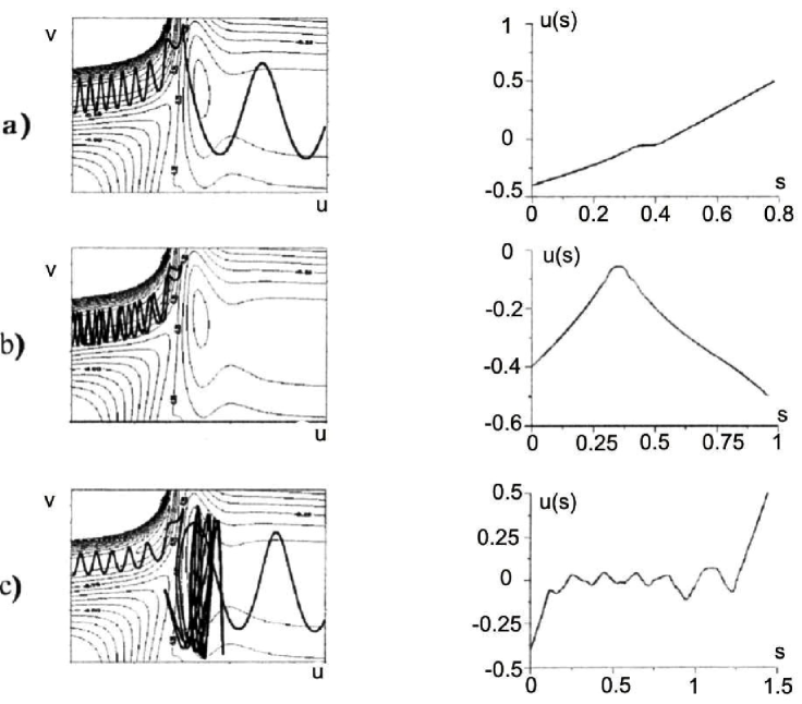
Figure 2: Geodesic trajectories and internal times depending on natural parameter $s$.

In Fig.2, three generating trajectories (or internal time) $u(s)$ and their corresponding $v(u)$ graphs are shown for different initial phases $\varphi$ of the trajectories. It is seen that the generating trajectories behave quite differently depending on the initial phase $\varphi$ for fixed energy $E$. Panel a) in Fig.2 shows a direct exchange reaction to which corresponds a monotone, but not uniformly changing, internal time (as a function of the natural parameter $s$ (usual time). Panel b) shows a non-reactive trajectory to which corresponds non-monotone internal time. In panel c) the geodesic trajectory again describes the exchange reaction which here goes via a resonance $(ABC)^{\ast}$ state and for which the dependence of $u$ on the parameter $s$ is complicated.

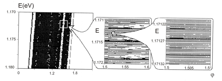
Figure 3: Chaotic map of initial values of the total energy $E$ and initial phase $\varphi$ for passed through (white points) and reflected back (black points) geodesic trajectories.

Now the main task is the investigation of the behavior of the geodesic trajectory flow. Numerical calculations shows, that for initial values corresponding to the chaotic regions mentioned above, the main Lyapunov exponent is positive and grows fast. The last fact points to exponential divergence of geodesic trajectories.

In Fig.3, the white points in initial parameter space correspond to the transition from the reactant ($R_{(in)}^{2}$ subspace) to product regions ($R_{(out)}^{2}$ subspace), while the black points correspond to the reflection back to the product region. The distribution of black and white points depend on energy and initial phase, for fixed initial vibrational coordinate $v_{0}$, and shows an irregular behavior. Recall that $v_{0}$ is an average equilibrium distance between bound particles $B$ and $C$ in the ground ($n=0$, where $n$-is a vibrational quantum number) state. Note that qualitatively the same picture we get for $v_{n}$ (equilibrium distance on excited quantum stat $n$). One can see from the results of calculations that the structure of chaotic behavior region is self-similar with respect to scale transformation.

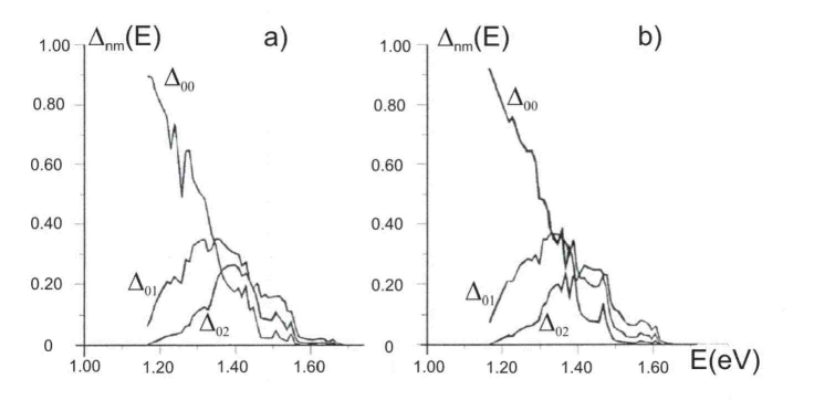
Figure 4: (a) - dependencies of transition probabilities $\Delta_{00},\,\Delta_{01}$ and $\Delta_{02}$ on energy $E$ for fixed phase $\varphi$; (b) - the same dependencies, but calculated for the other (slightly differing from the first one) fixed phase $\varphi_{a}-\varphi_{b}=10^{-5}$.

Let us consider the influence of chaotic behavior of the classical problem in Fig.4, which show the dependence on energy $E$ of over-barrier transition probabilities in the $Li+FH$ system for fixed phases $\varphi_{i}$ and equilibrium distance $v_{n}$. It can be seen that a small change in initial phase significantly changes the dependencies. In this connection the difficult problem arises to find a measure for the space (map) of passed through and reflected back geodesic trajectories. To calculate the probability for a specific quantum transition at an energy $E$, one has to average the corresponding quantum probability with respect to $\bigl{(}E,\varphi\bigr{)}$ within the range $[\Delta{E},\Delta{\varphi}=2\pi]$, where $\Delta{E}$ is a small interval of energies near $E$ and $\Delta{\varphi}=2\pi$ is the period of the values for the initial vibrational phase. The procedure of the averaging consists of that square $[\Delta{E}\times 2\pi]$ is divided by $N\gg 1$ rectangles, each of them having some phase point $\varphi_{i}$ inside. Then each rectangle is subdivided by the grid with $M_{i}=[l_{i}\times k_{i}]$ nodes, $l_{i}$ and $k_{i}$ being the number of breaking points for $\Delta{E}$ and $2\pi/N$ intervals respectively.

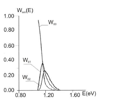
Figure 5: The transition probabilities after averaging with respect on phase distribution $\sigma(\varphi)$.

Probability for geodesic trajectory (generating trajectory) to pass through the $i$-th rectangle is calculated by the formula:

$$\sigma(\varphi_{i},E)=\lim_{l_{i},k_{i}\to\infty}N_{i}/M_{i},$$ (24)

where $N_{i}$ counts how many times the generating trajectory passes through into subspace $R^{2}_{(in)}$. Exchange reaction probability is then calculated as a limit of sum:

$$W_{\,n\to m}=\lim_{N\to\infty}\biggl{\{}\frac{\sum_{i=1}^{N}\sigma(\varphi_{i})\big{|}S_{\,n\to m}(\varphi_{i},E)\bigr{|}^{2}}{\sum_{i=1}^{N}\sigma(\varphi_{i})}\biggr{\}}=\frac{\int_{0}^{2\pi}\sigma(\varphi)\Delta_{n\,m}(\varphi,E)d\varphi}{\int_{0}^{2\pi}\sigma(\varphi)d\varphi}.$$ (25)

Particularly using (25) for reacting system $Li+(FH)\to(LiFH)^{\ast}\to(LiF)+H$ we can calculate transition probabilities see Fig.5.

IV conclusion

The $3D$ quantum theory Eq.s (12) and (18) was constructed, which described the classical permissible $P^{2}(u,v,\theta)>0$ reactive scattering in the three-body system with taking into account the influence of classical non-integrability on the quantum dynamics. By means of numerical modelling of collinear reacting system $Li+(FH)_{n}\to(LiFH)^{\ast}\to(LiF)_{m}+H$ it was shown that when chaotic region in phase space of classical system is larger than the quantum sell volume in the corresponding quantum system chaos is generated too. The calculations which are made for reacting collinear systems $O+N_{2},\,N+N_{2},\,N+O_{2},\,N+O_{2}$ show that the classical chaos is not enough developed and can’t generate the quantum chaos. However not excepting that these systems can be quantum chaotic in the $3D$ scattering case. Moreover we are sure that all $3D$ three-body scattering systems in more or less degrees are chaotic.

Finally it is necessary to note that developed approach to give a chance by defined conditions pass to $R$, $P$ and $Q$ regions of motion. When classical chaos is absent or developed insufficiently strong this approach coincides with standard quantum representation.

V Acknowledgments

This work partially was supported by INTAS Grant No. 03-51-4000, Armenian Science Research Council and Swedish Science Research Council.

References

- (1) A. Einstein, Zum Quantensatz von Sommerfeld und Epstein, Vehr. Dtsch. Phys. Ges., 19, 82, (1917).
- (2) M. C. Gutzwiller, Chaos in Class. and Quantum Mechanics, Springer, Berlin, (1990).
- (3) T. A. Brody et al., Rev. Mod. Phys. 53, (1981) 385.
- (4) H. Friedrich, D. Wintgen, Phys. Rep. 183, (1989) 37.
- (5) L. Nemes, Acta Phys. Hung. 73 (1993) 95.
- (6) V. Milner et al., Phys. Rev. Lett. 86 (2001) 1514.
- (7) N. Friedman, A. Kaplan, D. Carasso, N. Davidson, Phys. Rev. Lett. 86 (2001) 1518.
- (8) C. Dembrowski et al., Phys. Rev. Lett. 86 (2001) 3284.
- (9) S. W. McDonald, A. N. Kaufman, Phys. Rev. Lett. 42 (1979) 1189.
- (10) E. J. Heller, Phys. Rev. Lett. 53 (1984) 1515.
- (11) I. Hamilton and P. J. Brumer, Chem. Phys. 82, (1985) 1937.
- (12) D. M. Wardlaw and R.A. Marcus, Adv. Chem. Phys. 70-1, 231 (1988).
- (13) Z. Kovacs, L. Wiesenfeld, Phys. Rev. E. 51, (1995) 5476.
- (14) E. Ott and T. Tel, Chaos 3, (1993) 417.
- (15) U. Smilansky, Chaos and Quantum Physics, Ed. by M. J. Giannoni, A. Varos, and J. Zinn-Justin (north-Holland, Amsterdam, 1991), p. 371.
- (16) H. J. Stöckmann and J. Stein, Phys. Rev. Lett. 64, (1990) 1255.
- (17) E. Dorn and U. Smilansky, ibid 68, (1992) 1255.
- (18) G. Nyman and Yu Hua-Gen, Rep. Prog. Phys. 63, (2000) 1001.
- (19) A. V. Bogdanov et al., AMS/IP Studies in Adv. Math., 13, (1999) 69.
- (20) L. M. Delves, Nuclear Phys., 9, (1959) 391.
- (21) L. M. Smith, J. Chem. Phys., 31, (1959) 1352.
- (22) R. A. Marcus, J. Chem. Phys., 45, (1966) 4493.
- (23) J. Light, Adv. Chem. Phys., 19, (1971) 1.
- (24) A. S. Gevorkyan, G. Balint-Kurti and G. Nyman, arXiv:physics/0607093.
- (25) G. G. Balint-Kurti, L. F. sti-Molnr and A. Brown, Phys. Chem., 3, (2001) 702.
- (26) E. Hoft, J. Proc., of National Acad. of Sciences of USA, 18, (1932) 93.
- (27) N. S. Krylov, Studies on Foundation of Statistical Mechanics, Publ. AN SSSR, Leningrad, 1950.
- (28) A. Katok, Hassenblatt B., Introduction to the Modern Theory of Dynamical Systems, Cambridge University Press, 1996.
- (29) P. Honvault, J.-M. Launay, Chem. Phys. Lett. 329, (2000) 233-238.
- (30) F. Haake, Quantum Signatures of Chaos, (Springer-Verlag, Heidelberg, 2001).
- (31) M. L. Mehta, Random Matrices, Academic Press, New York, 1991.
- (32) J. S. Carter, J. N. Murrel, Physics, 41, 567, 1980.