Topological Quantum Compiling

Abstract

A method for compiling quantum algorithms into specific braiding patterns for nonabelian quasiparticles described by the so-called Fibonacci anyon model is developed. The method is based on the observation that a universal set of quantum gates acting on qubits encoded using triplets of these quasiparticles can be built entirely out of three-stranded braids (three-braids). These three-braids can then be efficiently compiled and improved to any required accuracy using the Solovay-Kitaev algorithm.

I Introduction

The requirements for realizing a fully functioning quantum computer are daunting. There must be a scalable system of qubits which can be initialized and individually measured. It must be possible to enact a universal set of quantum gates on these qubits. And all this must be done with sufficient accuracy so that quantum error correction can be used to prevent decoherence from spoiling any computation.

The problems of error and decoherence are particularly difficult ones for any proposed quantum computer. While the states of classical computers are typically stored in macroscopic degrees of freedom which have a built-in redundancy and thus are resistant to errors, building similar redundancy into quantum states is less natural. To protect quantum information it is necessary to encode it using quantum error correcting code states.shor ; steane These states are highly entangled, and have the property that code states corresponding to different logical qubit states can be distinguished from one another only by global (“topological”) measurements. Unlike states whose macroscopic degrees of freedom are effectively classical (think of the magnetic moment of a small part of a hard drive), such highly entangled “topologically degenerate” states do not typically emerge as the ground states of physical Hamiltonians. One route to fault-tolerant quantum computation is therefore to build the encoding and fault-tolerant gate protocols into the “software” of the quantum computer.aharonov

A remarkable recent development in the theory of quantum computation which directly addresses these issues has been the realization that certain exotic states of matter in two space dimensions, so-called nonabelian states, may provide a natural medium for storing and manipulating quantum information.kitaev ; freedman1 ; freedman2 ; freedmanbams In these states, localized quasiparticle excitations have quantum numbers which are in some ways similar to ordinary spin quantum numbers. However, unlike ordinary spins, the quantum information associated with these quantum numbers is stored globally, throughout the entire system, and so is intrinsically protected against decoherence. Furthermore, these quasiparticles satisfy so-called nonabelian statistics. This means that when two quasiparticles are adiabatically moved around one another, while being kept sufficiently far apart, the action on the Hilbert space is represented by a unitary matrix which depends only on the topology of the path used to carry out the exchange. Topological quantum computation can then be carried out by moving quasiparticles around one another in two space dimensions.kitaev ; freedman1 The quasiparticle world-lines form topologically nontrivial braids in three (= 2 + 1) dimensional space-time, and because these braids are topologically robust (i.e., they cannot be unbraided without cutting one of the strands) the resulting computation is protected against error.

Nonabelian states are expected to arise in a variety of quantum many-body systems, including spin systems,fendley ; nayak ; levin rotating Bose gases,cooper and Josephson junction arrays.doucot Of those states which have actually been experimentally observed, the most likely to possess nonabelian quasiparticle excitations are certain fractional quantum Hall states. Moore and Readmooreread were the first to propose that quasiparticle excitations which obey nonabelian statistics might exist in the fractional quantum Hall effect. Their proposal was based on the observation that the conformal blocks associated with correlation functions in the conformal field theory describing the two-dimensional Ising model could be interpreted as quantum Hall wave functions. These wave functions describe both the ground state of a half-filled Landau level of spin-polarized electrons, as well as states with some number of fractionally charged quasihole excitations (charge = $e/4$). The particular ground state this construction produces, the so-called Pfaffian, or Moore-Read state, is considered the most likely candidate for the observed fractional quantum Hall state at Landau level filling fraction $\nu=5/2$ ($\nu=1/2$ in the second Landau level).morf ; rezayi00

In this conformal field theory construction, states with four or more quasiholes present correspond to finite-dimensional conformal blocks, and so the corresponding wave functions form a finite-dimensional Hilbert space. The monodromy — or braiding properties — of these conformal blocks are then assumed to describe the unitary transformations acting on the Hilbert space produced by adiabatically braiding quasiholes around one another.mooreread Explicit wave functions for these states were worked out in Ref. nayakwilczek, , and the nonabelian braiding properties have been verified numerically in Ref. simon03, . In an alternate approach, the Moore-Read state can be viewed as a composite fermion superconductor in a so-called “weak pairing” $p_{x}+ip_{y}$ phase.readgreen In this description, the finite-dimensional Hilbert space arises from zero energy solutions of the Bogoliubov-DeGennes equations in the presence of vortices,readgreen and the vortices themselves are nonabelian quasiholes whose braiding properties have been shown to agree with the conformal field theory result.ivanov ; stern Recently, a number of experiments have been proposed to directly probe the nonabelian nature of these excitations.dassarma05 ; stern06 ; bonderson06 ; hou06

Unfortunately, the braiding properties of quasihole excitations in the Moore-Read state are not sufficiently rich to carry out purely topological quantum computation, although “partially” topological quantum computation using a mixture of topological and non-topological gates has been shown to be possible.bravyi ; freedman3 However, Read and Rezayireadrezayi have shown that the Moore-Read state is just one of a sequence of states labeled by an index $k$ corresponding to electrons at filling fractions $\nu=k/(2+k)$, with $k=1$ corresponding to the $\nu=1/3$ Laughlin state and $k=2$ to the Moore-Read state. The wavefunctions for these states can be written as correlation functions in the $Z_{k}$ parafermion conformal field theory,readrezayi and the braiding properties of the quasihole excitations were worked out in detail in Ref. slingerland01, . There it was shown that the quasiholes are described by the $SU(2)_{k}$ Chern-Simons-Witten (CSW) theories, up to overall abelian phase factors which are irrelevant for quantum computation. More recently, explicit quasihole wave functions have been worked out for the $k=3$ Read-Reazyi state,ardonne with results consistent with the predicted $SU(2)_{3}$ braiding properties. The elementary braiding matrices for the $SU(2)_{k}$ CSW theory for $k=3$ and $k\geq 5$ have been shown to be sufficiently rich to carry out universal quantum computation, in the sense that any desired unitary operation on the Hilbert space of $N$ quasiparticles, with $N\geq 3$ for $k\geq 3$, $k\neq 4,8$, and $N\geq 4$ for $k=8$, can be approximated to any desired accuracy by a braid.freedman1 ; freedman2

The main purpose of this paper is to give an efficient method for determining braids which can be used to carry out a universal set of a quantum gates (i.e. single-qubit rotations and controlled-NOT gates) on encoded qubits for the case $k=3$, thought to be physically relevant for the experimentally observedxia $\nu=12/5$ fractional quantum Hall effectreadrezayi ; rezayiread ($\nu=12/5$ corresponds to $\nu=2/5$ in the second Landau level, and this is the particle-hole conjugate of $\nu=3/5$ corresponding to $k=3$). We refer to the process of finding such braids as “topological quantum compiling” since these braids can then be used to translate a given quantum algorithm into the “machine code” of a topological quantum computer. This is analogous to the action of an ordinary compiler which translates instructions written in a high level programming language into the machine code of a classical computer.

It should be noted that the proof of universality for $SU(2)_{3}$ quasiparticles is a constructive one,freedman1 ; freedman2 and therefore, as a matter of principle, it provides a prescription for compiling quantum gates into braids. However, in practice, for two-qubit gates (such as controlled-NOT) this prescription, if followed straightforwardly, is prohibitively difficult to carry out, primarily because it involves searching the space of braids with six or more strands. We address this difficulty by dividing our two-qubit gate constructions into a series of smaller constructions, each of which only involves searching the space of three-stranded braids (three-braids). The required three-braids then can be found efficiently and used to construct the desired two-qubit gates. This “divide and conquer” approach does not, in general, yield the most accurate braid of a given length which approximates a desired quantum gate. However, we believe that it does yield the most accurate (or at least among the most accurate) braids which can be obtained for a given fixed amount of classical computing power.

This paper is organized as follows. In Sec. II we review the basic properties of the $SU(2)_{k}$ Hilbert space, and show that the case $SU(2)_{3}$ is, for our purposes, equivalent to the case $SO(3)_{3}$ – the so-called Fibonacci anyon model. Section III then presents a quick review of the mathematical machinery needed to compute with Fibonacci anyons. In Sec. IV we outline how, in principle, these particles can be used to encode qubits suitable for quantum computation. Section V then describes how to find braiding patterns for three Fibonacci anyons which can be used to carry out any allowed operation on the Hilbert space of these quasiparticles to any desired accuracy, thus effectively implementing the procedure given in Ref. freedman1, for carrying out single-qubit rotations. In Sec. VI we discuss the more difficult case of two-qubit gates, and give two classes of explicit gate constructions — one, first discussed by the authors in Ref. bonesteel05, , in which a pair of quasiparticles from one qubit is “woven” through the quasiparticles in the second qubit, and another, presented here for the first time, in which only a single quasiparticle is woven. Finally, in Sec. VII we address the question of to what extent the constructions we find are special to the $k=3$ case, and in Sec. VIII we summarize our results.

II Fusion Rules and Hilbert Space

Consider a system with quasiparticle excitations described by the $SU(2)_{k}$ CSW theory. It is convenient to describe the properties of this system using the so-called quantum group language.slingerland01 The relevant quantum groups are “deformed” versions of the representation theory of $SU(2)$, i.e. the theory of ordinary spin, and much of the intuition for thinking about ordinary spin can be carried over to the quantum group case.

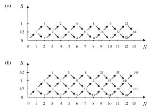
Figure 1: Bratteli diagrams for $SU(2)_{k}$ for (a) $k=2$ and (b) $k=3$. Here $N$ is the number of $q$-spin 1/2 quasiparticles and $S$ is the total $q$-spin of those quasiparticles. The number at a given $(N,S)$ vertex of each diagram indicates the number of paths to that vertex starting from the $(0,0)$ point. This number gives the dimensionality of the Hilbert space of $N$ $q$-spin 1/2 quasiparticles with total $q$-spin $S$.

In the quantum group description of an $SU(2)_{k}$ CSW theory, each quasiparticle has a half-integer $q$-deformed spin ($q$-spin) quantum number. Just as for ordinary spin, there are rules for combining $q$-spin known as fusion rules. The fusion rules for the $SU(2)_{k}$ theory are similar to the usual triangle rule for adding ordinary spin, except that they are truncated so that there are no states with total $q$-spin $>k/2$. Specifically, the fusion rules for the level $k$ theory are,fuchsbook

$$s_{1}\otimes s_{2} = |s_{1}-s_{2}|\oplus|s_{1}-s_{2}|+1\oplus\ldots$$ (1)

$$\ \ \ \ \ \ldots\oplus\min(s_{1}+s_{2},k-s_{1}-s_{2}).$$

Note that in the quantum group description of nonabelian anyons, states are distinguished only by their total $q$-spin quantum numbers. The $q$-deformed analogs of the $S_{z}$ quantum numbers are physically irrelevant — there is no degeneracy associated with them, and they play no role in any computation involving braiding.slingerland01 The situation is somewhat analogous to that of a collection of ordinary spin-1/2 particles in which the only allowed operations, including measurement, are rotationally invariant and hence independent of $S_{z}$, as is the case in exchange-based quantum computation.divincenzo

The fusion rules of the $SU(2)_{k}$ theory fix the structure of the Hilbert space of the system. For a collection of quasiparticles with $q$-spin 1/2, a useful way to visualize this Hilbert space is in terms of its so-called Bratteli diagram. This diagram shows the different fusion paths for $N$ $q$-spin 1/2 quasiparticles in which these quasiparticles are fused, one at a time, going from left to right in the diagram. Bratteli diagrams for the cases $k=2$ and $k=3$ are shown in Fig. 1.

The dimensionality of the Hilbert space for $N$ $q$-spin 1/2 quasiparticles with total $q$-spin $S$ can be determined by counting the number of paths in the Bratteli diagram from the origin to the point $(N,S)$. The results of this path counting are also shown in Fig. 1, where one can see the well-known $2^{N/2-1}$ Hilbert space degeneracy for the $k=2$ (Moore-Read) case,mooreread ; nayakwilczek and the Fibonnaci degeneracy for the $k=3$ case.readrezayi

In this paper we will focus on the $k=3$ case, which is the lowest $k$ value for which $SU(2)_{k}$ nonabelian anyons are universal for quantum computation.freedman1 ; freedman2 In fact, we will show that two-qubit gates are particularly simple for this case. Before proceeding, it is convenient to introduce an important property of the $SU(2)_{3}$ theory, namely that the braiding properties of $q$-spin 1/2 quasiparticles are the same as those with $q$-spin 1 (up to an overall abelian phase which is irrelevant for topological quantum computation). This is a useful observation because the theory of $q$-spin 1 quasiparticles in $SU(2)_{3}$ is equivalent to $SO(3)_{3}$, a theory also known as the Fibonacci anyon theorypreskillnotes ; kuperberg — a particularly simple theory with only two possible values of $q$-spin, 0 and 1, for which the fusion rules are

$$0\otimes 0=0,\ \ \ \ \ 0\otimes 1=1\otimes 0=1,\ \ \ \ \ 1\otimes 1=0\oplus 1.$$ (2)

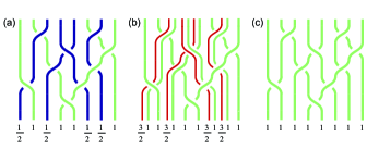
Figure 2: (color online). Graphical proof of the equivalence of braiding $q$-spin-1/2 and $q$-spin-1 objects for $SU(2)_{3}$. Part (a) shows a braiding pattern for a collection of objects, some having $q$-spin 1/2 and some having $q$-spin 1. Part (b) shows the same braiding pattern but with the $q$-spin-1/2 objects represented by $q$-spin 1 objects fused with $q$-spin-3/2 objects, which, for $SU(2)_{3}$, has a unique fusion channel. Finally, part (c) shows the same braid with the $q$-spin-3/2 objects removed. Because these $q$-spin-3/2 objects are effectively abelian for $SU(2)_{3}$, removing them from the braid will only result in an overall phase factor which will be irrelevant for quantum computing.

Here we give a rough proof of this equivalence. This proof is based on the fact that for $k=3$ the fusion rules involving $q$-spin 3/2 quasiparticles take the following simple form

$$\frac{3}{2}\otimes s = \frac{3}{2}-s.$$ (3)

The key observation is that since for $k=3$ the highest possible $q$-spin is 3/2, when fusing a $q$-spin-3/2 object with any other object (here we use the term object to describe either a single quasiparticle or a group of quasiparticles viewed as a single composite entity), the Hilbert space dimensionality does not grow. This implies that moving a $q$-spin-3/2 object around other objects can, at most, produce an overall abelian phase factor. While this phase factor may be important physically, particularly in determining the outcome of interference experiments involving nonabelian quasiparticles,dassarma05 ; stern06 ; bonderson06 ; hou06 it is irrelevant for quantum computing, and thus does not matter when determining braids which correspond to a given computation. Because (3) implies that a $q$-spin-1/2 object can be viewed as the result of fusing a $q$-spin-1 object with a $q$-spin-3/2 object, it follows that the braid matrices for $q$-spin-1/2 objects are the same as that for $q$-spin-1 objects up to an overall phase (as can be explicitly checked).

In fact, based on this argument we can make a stronger statement. Imagine a collection of $SU(2)_{3}$ objects which each have either $q$-spin 1 or $q$-spin 1/2. It is then possible to carry out topological quantum computation, even if we do not know which objects have $q$-spin 1 and which have $q$-spin 1/2. The proof is illustrated in Fig. 2. Figure 2(a) shows a braiding pattern for a collection of objects, some of which have $q$-spin 1/2 and some of which have $q$-spin 1. Fig. 2(b) then shows the same braiding pattern, but now all objects with $q$-spin 1/2 are represented by objects with $q$-spin 1 fused to objects with $q$-spin 3/2. Because, as noted above, the $q$-spin 3/2 objects have trivial (abelian) braiding properties, the unitary transformation produced by this braid is the same, up to an overall abelian phase, as that produced by braiding nothing but $q$-spin 1 objects, as shown in Fig. 2(c). It follows that provided one can measure whether the total $q$-spin of some object belongs to the class $1\equiv\{1,1/2\}$ or the class $0\equiv\{0,3/2\}$ — something which should, in principle, be possible by performing interference experiments as described in Refs. sb, and slingerland, — then quantum computation is possible, even if we do not know which objects have $q$-spin 1/2 and which have $q$-spin 1.

III Fibonacci Anyon Basics

Having reduced the problem of compiling braids for $SU(2)_{3}$ to compiling braids for $SO(3)_{3}$, i.e. Fibonacci anyons, it is useful for what follows to give more details about the mathematical structure associated with these quasiparticles. For an excellent review of this topic see Ref. preskillnotes, , and for the mathematics of nonabelian particles in general see Ref. kitaev2, .

Note that for the rest of this paper, except for Sec. VII, it should be understood that each quasiparticle is a $q$-spin 1 Fibonacci anyon. It should also be understood that from the point of view of their nonabelian properties quasihole excitations are also $q$-spin 1 Fibonacci anyons, even though they have opposite electric charge and give opposite abelian phase factors when braided. Because it is the nonabelian properties which are relevant for topological quantum computation, for our purposes quasiparticles and quasiholes can be viewed as identical nonabelian particles. Unless it is important to distinguish between the two (as when we discuss creating and fusing quasiparticles and quasiholes in Sec. IV) we will simply use the terms quasiparticle or Fibonacci anyon to refer to either excitation.

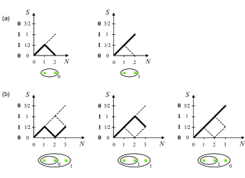
Figure 3: (color online). Basis states for the Hilbert space of (a) two and (b) three Fibonacci anyons. $SU(2)_{3}$ Bratteli diagrams showing fusion paths corresponding to the basis states for the Hilbert space of two and three $q$-spin 1/2 quasiparticles are shown. The $q$-spin axes on these diagrams are labeled both by the $SU(2)_{3}$ $q$-spin quantum numbers 0, 1/2, 1 and 3/2 and, to the left of these in bold, the corresponding Fibonacci $q$-spin quantum numbers $0\equiv\{0,3/2\}$ and $1\equiv\{1/2,1\}$. Beneath each Bratteli diagram the same state is represented using a notation in which dots correspond to Fibonacci anyons, and groups of Fibonacci anyons enclosed in ovals labeled by $q$-spin quantum numbers are in the corresponding $q$-spin eigenstates.

Figure 3 establishes some of the notation for representing Fibonacci anyons which will be used in the rest of the paper. This figure shows $SU(2)_{3}$ Bratteli diagrams in which the $q$-spin axis is labeled both by the $SU(2)_{3}$ $q$-spin quantum numbers and, in boldface, the corresponding Fibonacci $q$-spin quantum numbers, i.e. 0 for $\{0,3/2\}$ and 1 for $\{1/2,1\}$. In Fig. 3(a) Bratteli diagrams showing fusion paths corresponding to two basis states spanning the two-dimensional Hilbert space of two Fibonacci anyons are shown. Beneath each Bratteli diagram an alternate representation of the corresponding state is also shown. In this representation dots correspond to Fibonacci anyons and ovals enclose collections of Fibonacci anyons which are in $q$-spin eigenstates whenever the oval is labeled by a total $q$-spin quantum number. (Note: If the oval is not labeled, it should be understood that the enclosed quasiparticles may not be in a $q$-spin eigenstate).

In the text we will use the notation $\bullet$ to represent a Fibonacci anyon, and the ovals will be represented by parentheses. In this notation, the two states shown in Fig. 3(a) are denoted $(\bullet,\bullet)_{0}$ and $(\bullet,\bullet)_{1}$.

Fig. 3(b) shows Bratteli diagram, again with both $SU(2)_{3}$ and Fibonacci quantum numbers, with fusion paths which this time correspond to three basis states of the three-dimensional Hilbert space of three Fibonacci anyons. Beneath these diagrams the “oval” representations of these three states are also shown, which in the text will be represented $((\bullet,\bullet)_{0},\bullet)_{1}$, $((\bullet,\bullet)_{1},\bullet)_{1}$ and $((\bullet,\bullet)_{1},\bullet)_{0}$.

In addition to fusion rules, all theories of nonabelian anyons possess additional mathematical structure which allows one to calculate the result of any braiding operation. This structure is characterized by the $F$ (fusion) and $R$ (rotation) matrices.preskillnotes ; kitaev2 ; mooreseiberg

To define the $F$ matrix, note that the Hilbert space of three Fibonacci anyons is spanned both by the three states labeled $((\bullet,\bullet)_{a},\bullet)_{c}$, and the three states labeled $(\bullet,(\bullet,\bullet)_{b})_{c}$. The $F$ matrix is the unitary transformation which maps one of these bases to the other,

$$\left(\bullet,\left(\bullet,\bullet\right)_{a}\right)_{c}=\sum_{b}F^{c}_{ab}\left(\left(\bullet,\bullet\right)_{b},\bullet\right)_{c},$$ (4)

and has the form

$$F=\left(\begin{array}[]{cc|c}\tau&\sqrt{\tau}&\\ \sqrt{\tau}&-\tau&\\ \hline\cr&&1\end{array}\right),$$ (8)

where $\tau=(\sqrt{5}-1)/2$ is the inverse of the golden mean. In this matrix the upper left 2$\times$2 block, $F^{1}_{ab}$, acts on the two-dimensional total $q$-spin 1 sector of the three-quasiparticle Hilbert space and the lower right matrix element, $F^{0}_{11}=1$, acts on the unique total $q$-spin 0 state. Note that this $F$ matrix can be applied to any three objects which each have $q$-spin 1, where each object can consist of more than one Fibonacci anyon. Furthermore, if one considers three objects for which one or more of the objects has $q$-spin 0, then the state of these objects is uniquely determined by the total $q$-spin of all three, and in this case the $F$ matrix is trivially the identity. Thus, for the case of Fibonacci anyons, the matrix (8) is all that is needed to make arbitrary basis changes for any number of Fibonacci anyons.

The $R$ matrix gives the phase factor produced when two Fibonacci anyons are moved around one another with a certain sense. One can think of these phase factors as the $q$-deformed versions of the $-1$ or $+1$ phase factors one obtains when interchanging two ordinary spin-1/2 quasiparticles when they are in a singlet or triplet state, respectively. This phase factor depends on the overall $q$-spin of the two quasiparticles involved in the exchange, so for Fibonacci anyons there are two such phase factors which are summarized in the $R$ matrix,

$$R=\left(\begin{array}[]{cc}e^{-i4\pi/5}&0\\ 0&e^{i3\pi/5}\end{array}\right).$$ (11)

Here the upper left and lower right matrix elements are, respectively, the phase factor that two Fibonacci anyons acquire if they are interchanged in a clockwise sense when they have total $q$-spin 0 or $q$-spin 1. Again, this matrix also applies if we exchange two objects that both have total $q$-spin 1, even if these objects consist of more than one Fibonacci anyon. And if one or both objects has $q$-spin 0, the result of this interchange is the identity. Again we emphasize that in the $k=3$ Read-Rezayi state, there will be additional abelian phases present, which may have physical consequences for some experiments, but which will be irrelevant for topological quantum computation.

Typically the sequence of $F$ and $R$ matrices used to compute the unitary operation produced by a given braid is not unique. To guarantee that the result of any such computation is independent of this sequence, the $F$ and $R$ matrices must satisfy certain consistency conditions. These consistency conditions, the so-called pentagon and hexagon equations,preskillnotes ; kitaev2 ; mooreseiberg are highly restrictive, and, in fact, for the case of Fibonacci anyons essentially fix the $F$ and $R$ matrices to have the forms given above (up to a choice of chirality, and Abelian phase factors which are again irrelevant to our purposes here).preskillnotes

Finally, we point out an obvious, but important, consequence of the structure of the $F$ and $R$ matrices. When interchanging any two quasiparticles which are part of a larger set of quasiparticles with a well-defined total $q$-spin quantum number, this total $q$-spin quantum number will not change.

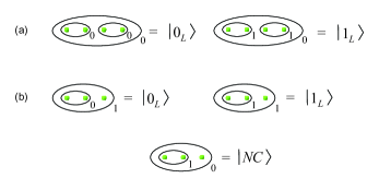
Figure 4: (color online). (a) Four-quasparticle and (b) three-quasiparticle qubit encodings for Fibonacci anyons. Part (a) shows two states which span the Hilbert space of four quasiparticles with total $q$-spin 0 which can be used as the logical $|0_{L}\rangle$ and $|1_{L}\rangle$ states of a qubit. Part (b) shows two states spanning the Hilbert space of three quasiparticles with total $q$-spin 1 which can also be used as logical qubit states $|0_{L}\rangle$ and $|1_{L}\rangle$. This three-quasiparticle qubit can be obtained by removing the rightmost quasiparticle from the two states shown in (a). The third state shown in Part (b), labeled $|NC\rangle$ for “noncomputational”, is the unique state of three quasiparticles which has total $q$-spin 0.

IV Qubit Encoding and General Computation Scheme

Before proceeding, it will be useful to have a specific scheme in mind for how one might actually carry out topological quantum computation with Fibonacci anyons. Here we follow the scheme outlined in Ref. freedmanbams, , which, for completeness, we briefly review below.

The computer can be initialized by pulling quasiparticle-quasihole pairs out of the “vacuum”, (by vacuum we mean the ground state of the $k=3$ Read-Rezayi state or any other state which supports Fibonacci anyon excitations). Each such pair will consist of two $q$-spin 1 excitations in a state with total $q$-spin 0, i.e. the state $(\bullet,\bullet)_{0}$. In principle, this pair can also exist in a state with total $q$-spin 1, provided there are other quasiparticles present to ensure the total $q$-spin of the system is 0, so one can imagine using this pair as a qubit. However, it is impossible to carry out arbitrary single-qubit operations by braiding only the two quasiparticles forming such a qubit — this braiding never changes the total $q$-spin of the pair, and so only generates rotations about the $z$-axis in the qubit space.

For this reason it is convenient to encode qubits using more than two Fibonacci anyons. Thus, to create a qubit, two quasiparticle-quasihole pairs can be pulled out of the vacuum. The resulting state is then $((\bullet,\bullet)_{0},(\bullet,\bullet)_{0})_{0}$ which again has total $q$-spin 0. The Hilbert space of four Fibonacci anyons with total $q$-spin 0 is two dimensional, with basis states, which we can take as logical qubit states, $|0_{L}\rangle=((\bullet,\bullet)_{0},(\bullet,\bullet)_{0})_{0}$ and $|1_{L}\rangle=((\bullet,\bullet)_{1},(\bullet,\bullet)_{1})_{0}$, (see Fig 4(a)). The state of such a four-quasiparticle qubit is determined by the total $q$-spin of either the rightmost or leftmost pair of quasiparticles. Note that the fusion rules (2) imply that the total $q$-spin of these two pairs must be the same because the total $q$-spin of all four quasiparticles is 0.

For this encoding, in addition to the two-dimensional computational qubit space of four quasiparticles with total $q$-spin 0, there is a three-dimensional noncomputational Hilbert space of states with total $q$-spin 1 spanned by the states $((\bullet,\bullet)_{0},(\bullet,\bullet)_{1})_{1}$, $((\bullet,\bullet)_{1},(\bullet,\bullet)_{0})_{1}$ and $((\bullet,\bullet)_{1},(\bullet,\bullet)_{1})_{1}$. When carrying out topological quantum computation it is crucial to avoid transitions into this noncomputational space.

Fortunately, single-qubit rotations can be carried out by braiding quasiparticles within a given qubit and, as discussed in Sec. III, such operations will not change the total $q$-spin of the four quasiparticles involved. Single-qubit operations can therefore be carried out without any undesirable transitions out of the encoded computational qubit space.

Two-qubit gates, however, will require braiding quasiparticles from different qubits around one another. This will in general lead to transitions out of the encoded qubit space. Nevertheless, given the so-called ”density” result of Ref. freedman2, it is known that, as a matter of principle, one can always find two-qubit braiding patterns which will entangle the two qubits, and also stay within the computational space to whatever accuracy is required for a given computation. The main purpose of this paper is to show how such braiding patterns can be efficiently found.

Note that the action of braiding the two leftmost quasiparticles in a four-quasiparticle qubit (referring to Fig. 4(a)) is equivalent to that of braiding the two rightmost quasiparticles with the same sense. This is because as long as we are in the computational qubit space both the leftmost and rightmost quasiparticle pairs must have the same total $q$-spin, and so interchanging either pair will result in the same phase factor from the $R$ matrix. It is therefore not necessary to braid all four quasiparticles to carry out single-qubit rotations — one need only braid three.

In fact, one may consider qubits encoded using only three quasiparticles with total $q$-spin 1, as originally proposed in Ref. freedman1, . Such qubits can be initialized by first creating a four-quasiparticle qubit in the state $|0_{L}\rangle$, as outlined above, and then simply removing one of the quasiparticles. In this three-quasiparticle encoding, shown in Fig. 4(b), the logical qubit states can be taken to be $|0_{L}\rangle=((\bullet,\bullet)_{0},\bullet)_{1}$ and $|1_{L}\rangle=((\bullet,\bullet)_{1},\bullet)_{1}$. For this encoding there is just a single noncomputational state $|NC\rangle=((\bullet,\bullet)_{1},\bullet)_{0}$, also shown in Fig. 4(b). As for the four-quasiparticle qubit, when carrying out single-qubit rotations by braiding within a three-quasiparticle qubit the total $q$-spin of the qubit, in this case 1, remains unchanged and there are no transitions from the computational qubit space into the state $|NC\rangle$. However, just as for four-quasiparticle qubits, when carrying out two-qubit gates these transitions will in general occur and we must work hard to avoid them. Henceforth we will refer to these unwanted transitions as leakage errors.

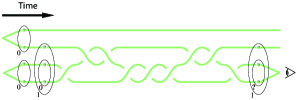
Figure 5: (color online). Space-time paths corresponding to the initialization, manipulation through braiding, and measurement of an encoded qubit. Two quasiparticle-quasihole pairs are pulled out of the vacuum, with each pair having total $q$-spin 0. The resulting state corresponds to a four-quasiparticle qubit in the state $|0_{L}\rangle$ (see Fig. 4(a)). After some braiding, the qubit is measured by trying to fuse the bottommost pair (in this case a quasiparticle-quasihole pair). If they fuse back into the vacuum the result of the measurement is $|0_{L}\rangle$, otherwise it is $|1_{L}\rangle$. Because only the three lower quasiparticles are braided, the encoded qubit can also be viewed as a three-quasiparticle qubit (see Fig. 4(b)) which is initialized in the state $|0_{L}\rangle$.

Note that, because each three-quasiparticle qubit has total $q$-spin 1, when more than one of these qubits is present the state of the system is not entirely characterized by the “internal” $q$-spin quantum numbers which determine the computational qubit states. It is also necessary to specify the state of what we will refer to as the “external fusion space” — the Hilbert space associated with fusing the total $q$-spin 1 quantum numbers of each qubit. When compiling braids for three-quasiparticle qubits it is crucial that the operations on the computational qubit space not depend on the state of this external fusion space — if they did, these two spaces would become entangled with one another leading to errors. Fortunately, we will see that it is indeed possible to find braids which do not lead to such errors.

For the rest of this paper (except Sec. VII) we will use this three-quasiparticle qubit encoding. It should be noted that any braid which carries out a desired operation on the computational space for three-quasiparticle qubits will carry out the same operation on the computational space of four-quasiparticle qubits, with one quasiparticle in each qubit acting as a spectator. The braids we find here can therefore be used for either encoding.

We can now describe how topological quantum computation might actually proceed, again following Ref. freedmanbams, . A quantum circuit consisting of a sequence of one- and two-qubit gates which carries out a particular quantum algorithm would first be translated (or “compiled”) into a braid by compiling each individual gate to whatever accuracy is required. Qubits would then be initialized by pulling quasiparticle-quasihole pairs out of the “vacuum”. These localized excitations would then be adiabatically dragged around one another so that their world-lines trace out a braid in three-dimensional space-time which is topologically equivalent to the braid compiled from the quantum algorithm. Finally, individual qubits would be measured by trying to fuse either the two rightmost or two leftmost excitations within them (referring to Fig. 4(a)) for four-quasiparticle qubits, or just the two leftmost excitations (referring to Fig. 4(b)) for three-quasiparticle qubits. If this pair of excitations consists of a quasiparticle and a quasihole (and it will always be possible to arrange this), then, if the total $q$-spin of the pair is 0, it will be possible for them to fuse back into the “vacuum”. However, if the total $q$-spin is 1 this will not be possible. The resulting difference in the charge distribution of the final state would then be measured to determine if the qubit was in the state $|0_{L}\rangle$ or $|1_{L}\rangle$. Alternatively, as already mentioned in Sec. II, interference experimentssb ; slingerland could be used to initialize and read out encoded qubits.

As a simple illustration, Fig. 5 shows a “computation” in which a four-quasiparticle qubit (which can also be viewed as a three-quasiparticle qubit if the top quasiparticle is ignored) is initialized by pulling quasiparticle-quasihole pairs out of the vacuum, a single-qubit operation is carried out by braiding within the qubit, and the final state of the qubit is measured by fusing a quasiparticle and quasihole together and observing the outcome.

V Compiling three-braids and single-qubit gates

We now focus on the problem of finding braids for three Fibonacci anyons (three-braids) which approximate any allowed unitary transformation on the Hilbert space of these quasiparticles. This is important not only because it allows one to find braids which carry out arbitrary single-qubit rotations,freedman1 but also because, as will be shown in Sec. VI, it is possible to reduce the problem of constructing braids which carry out two-qubit gates to that of finding a series of three-braids approximating specific operations.

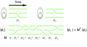
Figure 6: (color online). Elementary three-braids and the decomposition of a general three-braid into a series of elementary braids. The unitary operation produced by this braid is computed by multiplying the corresponding sequence of elementary braid matrices, $\sigma_{1}$ and $\sigma_{2}$ (see text) and their inverses, as shown. Here the (unlabeled) ovals represent a particular basis choice for the three-quasiparticle Hilbert space, consistent with that used in the text. In this and all subsequent figures which show braids, quasiparticles are aligned vertically, and we adopt the convention that reading from bottom to top in the figures corresponds to reading from left to right in expressions such as $((\bullet,\bullet)_{a},\bullet)_{c}$ in the text. It should be noted that these figures are only meant to represent the topology of a given braid. In any actual implementation of topological quantum computation, quasiparticles will certainly not be arranged in a straight line, and they will have to be kept sufficiently far apart while being braided to avoid lifting the topological degeneracy.

V.1 Elementary Braid Matrices

Using the $F$ and $R$ matrices, it is straightforward to determine the elementary braiding matrices that act on the three-dimensional Hilbert space of three Fibonacci anyons. If, as in Fig. 6, we take the basis states for the three-quasiparticle Hilbert space to be the states labeled $((\bullet,\bullet)_{a},\bullet)_{c}$ then, in the $ac=\{01,11,10\}$ basis, the matrix $\sigma_{1}$ corresponding to a clockwise interchange of the two bottommost quasiparticles in the figure (or leftmost in the $((\bullet,\bullet)_{a},\bullet)_{c}$ representation) is

$$\sigma_{1}=\left(\begin{array}[]{cc|c}e^{-i4\pi/5}&0&\\ 0&e^{i3\pi/5}&\\ \hline\cr&&e^{i3\pi/5}\end{array}\right),$$ (15)

where the upper left 2$\times$2 block acts on the total $q$-spin 1 sector ($|0\rangle_{L}$ and $|1\rangle_{L}$) of the three quasiparticles, and the lower right matrix element is a phase factor acquired by the $q$-spin 0 state ($|NC\rangle$). This matrix is easily read off from the $R$ matrix, since the total $q$-spin of the two quasiparticles being exchanged is well defined in this basis.

To find the matrix $\sigma_{2}$ corresponding to a clockwise interchange of the two topmost (or rightmost in the $((\bullet,\bullet)_{a},\bullet)_{c}$ representation) quasiparticles, we must first use the $F$ matrix to change bases to one in which the total $q$-spin of these quasiparticles is well defined. In this basis, the braiding matrix is simply $\sigma_{1}$, and so, after changing back to the original basis, we find

$$\sigma_{2}=F^{-1}\sigma_{1}F=\left(\begin{array}[]{cc|c}-\tau e^{-i\pi/5}&\sqrt{\tau}e^{-i3\pi/5}&\\ \sqrt{\tau}e^{-i3\pi/5}&-\tau&\\ \hline\cr&&e^{i3\pi/5}\end{array}\right).$$ (19)

The unitary transformation corresponding to a given three-braid can now be computed by representing it as a sequence of elementary braid operations and multiplying the corresponding sequence of $\sigma_{1}$ and $\sigma_{2}$ matrices and their inverses, as shown in Fig. 6.

If we are only concerned with single-qubit rotations, then we only care about the action of these matrices on the encoded qubit space with total $q$-spin 1, and not the total $q$-spin 0 sector corresponding to the noncomputational state. However, in our two-qubit gate constructions, various three-braids will be embedded into the braiding patterns of six quasiparticles, and in this case the action on the full three-dimensional Hilbert space does matter.

To understand this action note that $\sigma_{1}$ can be written

$$\sigma_{1}=\left(\begin{array}[]{c|c}\pm e^{-i\pi/10}\left(\begin{array}[]{cc}\pm e^{-i7\pi/10}&0\\ 0&\pm e^{i7\pi/10}\end{array}\right)&\\ \hline\cr&e^{i3\pi/5}\end{array}\right),~{}$$ (24)

where the upper $2\times 2$ block acting on the total $q$-spin 1 sector is an $SU(2)$ matrix, (i.e., a $2\times 2$ unitary matrix with determinant 1), multiplied by a phase factor of either $+e^{-i\pi/10}$ or $-e^{-i\pi/10}$, and the lower right matrix element, $e^{i3\pi/5}$, is the phase acquired by the total $q$-spin 0 state. The phase factor pulled out of the upper $2\times 2$ block is only defined up to $\pm 1$ because any $SU(2)$ matrix multiplied by $-1$ is also an $SU(2)$ matrix.

From (19) it follows that $\sigma_{2}$ can be written in a similar fashion, with the same phase factors. Each clockwise braiding operation then corresponds to applying an $SU(2)$ operation multiplied by a phase factor of $\pm e^{-i\pi/10}$ to the $q$-spin 1 sector, while at the same time multiplying the $q$-spin 0 sector by a phase factor of $e^{i3\pi/5}$. Likewise, each counterclockwise braiding operation corresponds to applying an $SU(2)$ operation multiplied by a phase factor of $\pm e^{+i\pi/10}$ to the $q$-spin 1 sector and a phase factor of $e^{-i3\pi/5}$ to the $q$-spin 0 sector.

We define the winding, $W(B)$, of a given three-braid $B$, to be the total number of clockwise interchanges minus the total number of counterclockwise interchanges. It then follows that the unitary operation corresponding to an arbitrary braid $B$ can always be expressed

$$U(B)=\left(\begin{array}[]{c|c}\pm e^{-iW(B)\pi/10}\>[SU(2)]&\\ \hline\cr&e^{i3W(B)\pi/5}\end{array}\right),$$ (27)

where $[SU(2)]$ indicates an $SU(2)$ matrix. Thus, for a given three-braid, the phase relation between the total $q$-spin 1 and total $q$-spin 0 sectors of the corresponding unitary operation is determined by the winding of the braid. We will refer to (27) often in what follows. It tells us precisely what unitary operations can be approximated by three-braids, and places useful restrictions on their winding.

V.2 Weaving and Brute Force Search

At this point it is convenient to restrict ourselves to a subclass of braids which we will refer to as weaves. A weave is any braid which is topologically equivalent to the space-time paths of some number of quasiparticles in which only a single quasiparticle moves. It was shown in Ref. simon06, that this restricted class of braids is universal for quantum computation, provided the unitary representation of the braid group is dense in the space of all unitary transformations on the relevant Hilbert space, which is the case for Fibonacci anyons.

Following Ref. simon06, we will borrow some weaving terminology and refer to the mobile quasiparticle (or collection of quasiparticles) as the “weft” quasiparticle(s) and the static quasiparticles as the “warp” quasiparticles.

One reason for focusing on weaves is that weaving will likely be easier to accomplish technologically than general braiding. This is true even if the full computation involves not just weaving a single quasiparticle, as was proposed in Ref. simon06, , but possibly weaving several quasiparticles at the same time in different regions of the computer — carrying out quantum gates on different qubits in parallel.

Considering weaves has the added (and more immediate) benefit of simplifying the problem of numerically searching for three-braids which approximate desired gates. For the full braid group, even on just three strands, there is a great deal of redundancy since braids which are topologically equivalent will yield the same unitary operation. Weaves, however, naturally provide a unique representation in which the warp strands are straight, and the weft weaves around them. There is therefore no trivial “double counting” of topologically equivalent weaves when one does a brute force numerical search of weaves up to some given length.

The unitary operations performed by weaving three quasiparticles in which the weft quasiparticle starts and ends in the middle position, will always have the form

$$U_{\rm weave}(\{n_{i}\})=\sigma_{1}^{n_{m}}\sigma_{2}^{n_{m-1}}\cdots\sigma_{1}^{n_{3}}\sigma_{2}^{n_{2}}\sigma_{1}^{n_{1}}.$$ (28)

Here the sequence of exponents $n_{2},n_{3}\cdots n_{m-1}$ all take their values from $\{\pm 2,\pm 4\}$, and $n_{1}$ and $n_{m}$ can take the values $\{0,\pm 2,\pm 4\}$. Because these exponents are all even, each factor in this sequence takes the weft quasiparticle all the way around one of the two warp quasiparticles either once or twice with either a clockwise or counterclockwise sense, returning it to the middle position. We allow $n_{1}$ and $n_{m}$ to be 0 to account for the possibility that the initial or final weaving operations could each be either $\sigma_{1}^{n}$ or $\sigma_{2}^{n}$ with $n=\pm 2$ or $\pm 4$. Note that we need only consider exponents $n_{i}$ up to $\pm 4$ (i.e., moving the weft quasiparticle at most two times around a warp quasiparticle) because of the fact that $\sigma_{i}^{10}=1$ for Fibonacci anyons, implying, e.g., $\sigma_{i}^{6}=\sigma_{i}^{-4}$. We define the length $L$ of such weaves to be equal to the total number of elementary crossings, thus $L=\sum_{i=1}^{m}|n_{i}|$.

We will also consider weaves in which the weft quasiparticle begins and/or ends at a position other than the middle. These possibilities can easily be taken into account by multiplying $U_{\rm weave}(\{n_{i}\})$, as defined in (28), by the appropriate factors of $\sigma_{1}$ or $\sigma_{2}$ on the right and/or left. Thus, for example, the unitary operation produced by a weave in which the weft quasiparticle starts in the top position and ends in the middle position can be written $U_{\rm weave}(\{n_{i}\})\sigma_{2}$, where, because of the extra factor of $\sigma_{2}$, the first braiding operations carried out by this weave will be $\sigma_{2}^{n}$ where $n$ is an odd power, $n=\pm 1,\pm 3$ or 5. This will weave the weft quasiparticle from the top position to the middle position after which $U_{\rm weave}$ will simply continue weaving this quasiparticle eventually ending with it in the middle position. (Note that by multiplying $U_{\rm weave}$ on the right by $\sigma_{2}$, and not $\sigma_{2}^{-1}$, we are not requiring the initial elementary braid to be clockwise, since $U_{\rm weave}$ may have $n_{1}=0$ and $n_{2}=-2$ or $-4$ so that the initial $\sigma_{2}$ is immediately multiplied by $\sigma_{2}$ to a negative power.) Similarly, the unitary operation produced by a weave in which the weft particle starts in the top position and ends in the bottom position can be written $\sigma_{1}U_{\rm weave}(\{n_{i}\})\sigma_{2}$, and so on.

To find a weave for which the corresponding unitary operation $U_{\rm weave}(\{n_{i}\})$ approximates a particular desired unitary operation, the most straightforward approach is to simply perform a brute force search over all weaves, i.e. all sequences $\{n_{i}\}$ as described above, up to a certain length $L$, in order to find the $U_{\rm weave}(\{n_{i}\})$ which is closest to the target operation. Here we will take as a measure of the distance between two operators $U$ and $V$ the operator norm distance $\epsilon(U,V)=||U-V||$ where $||O||$ is the operator norm, defined to be the square root of the highest eigenvalue of $O^{\dagger}O$. Again, if we are interested in fixing the relative phase of the total $q$-spin 1 and total $q$-spin 0 sectors then we would restrict the winding of the weaves so that the phases in (27) match those of the desired target gate.

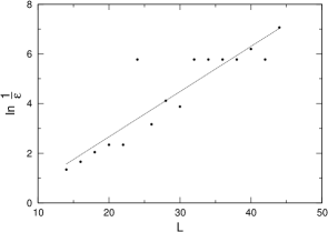
Figure 7: $\ln\frac{1}{\epsilon}$ vs. braid length $L$ for weaves approximating the gate $iX$. Here $\epsilon$ is the distance (defined in terms of operator norm) between $iX$ and the unitary transformation produced by a weave of length $L$ which best approximates it. The line is a guide to the eye.

For example, imagine our goal is to find a weave which approximates the unitary operation,

$$iX=\left(\begin{array}[]{cc|c}0&i&\\ i&0&\\ \hline\cr&&1\end{array}\right).$$ (32)

If the resulting weave were to be used only for a single-qubit operation, then we would only require that the weave approximate the upper left $2\times 2$ block of $iX$ up to an overall phase and we would not care about the phase factor appearing in the lower right matrix element. There would then be no constraint on the winding of the braid. However, for this example we will assume that this weave will be used in a two-qubit gate construction, for which the overall phase and/or the phase difference between the total $q$-spin 1 and total $q$-spin 0 sectors will matter.

In this case, by comparing $iX$ to (27), we see that the winding $W$ of any weave approximating $iX$ must satisfy $e^{i3\pi W/5}=1$ or $W=0$ (modulo 10). Results of a brute force search over weaves satisfying this winding requirement which approximate $iX$ are shown in Fig. 7. In this figure, $\ln\frac{1}{\epsilon}$ is plotted vs. braid length $L$, where $\epsilon$ is the minimum distance between $U_{\rm weave}$ and $iX$ for weaves of length $L$. It is expected that, for any such brute force search for weaves approximating a generic target operation, the length should scale with distance according to $L\sim\log\frac{1}{\epsilon}$, because the number of braids grows exponentially with $L$. The results shown in Fig. 7 are consistent with such logarithmic scaling.

All the brute force searches used to find braids in this paper are straightforward sequential searches, meant mainly to demonstrate proof of principle. No doubt more sophisticated brute force search methods (e.g. bidirectional search) could be used to perform deeper searches resulting in longer and more accurate braids. Nevertheless, the exponential growth in the number of braids with $L$ implies that finding optimal braids by any brute force search method will rapidly become infeasible as $L$ increases. Fortunately one can still systematically improve a given braid to any desired accuracy by applying the Solovay-Kitaev algorithm,kitaevbook ; nielsenbook which we now briefly review.

V.3 Implementation of the Solovay-Kitaev Algorithm for Braids

The general result of the Solovay-Kitaev theorem tells us that we can efficiently improve the accuracy of any given braid without the need to perform exhaustive brute force searches of ever improving accuracy.kitaevbook ; nielsenbook The essential ingredient in this procedure is an $\epsilon$-net — a discrete set of operators which in the present case correspond to finite braids up to some given length, with the property that for any desired unitary operator there exists an element of the $\epsilon$-net which is within some given distance $\epsilon_{0}$ of that operator. Provided $\epsilon_{0}$ is sufficiently small, the Solovay-Kitaev algorithm gives us a clever way to pick a finite number of braid segments out of the $\epsilon$-net and sew them together so that the resulting gate will be an approximation to the desired gate with improved accuracy.

The implementation of the Solovay-Kitaev algorithm we use here follows closely that described in detail in Refs. harrow, and dawson, . The first step of this algorithm is to find a braid which approximates the desired gate, $U$, by performing a brute force search over the $\epsilon$-net. Let $U_{0}$ denote the result of this search. Since we know that $\epsilon(U_{0},U)\leq\epsilon_{0}$ it follows that $C=UU_{0}^{-1}$ is an operator which is within a distance $\epsilon_{0}$ of the identity.

The next step is to decompose $C$ as a group commutator. This means that we find two unitary operators $A$ and $B$ for which $C=ABA^{-1}B^{-1}$. The unitary operators $A$ and $B$ are chosen so that their action on the computational qubit space corresponds to small rotations through the same angle but about perpendicular axes. For this choice, if $A$ and $B$ are then approximated by operators $A_{0}$ and $B_{0}$ in the $\epsilon$-net, it can readily be shown that the operator $C_{0}=A_{0}B_{0}A_{0}^{-1}B_{0}^{-1}$, will approximate $C$ to a distance of order $\epsilon_{0}^{3/2}$. It follows that the operator $U_{1}=A_{0}B_{0}A_{0}^{-1}B_{0}^{-1}U_{0}$ is an approximation to $U$ within a distance $\epsilon_{1}\simeq c\epsilon_{0}^{3/2}$, where $c$ is a constant which determines the size of the $\epsilon$-net needed to guarantee an improvement in accuracy.

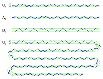
Figure 8: (color online). One iteration of the Solovay-Kitaev algorithm applied to finding a braid which approximates the operation $U=iX$. The braid $U_{0}$ is the result of a brute force search over weaves up to length 44 which best approximates the desired gate $U=iX$, with an operator norm distance between $U$ and $U_{0}$ of $\epsilon\simeq 8.5\times 10^{-4}$. The braids $A_{0}$ and $B_{0}$ are the results of similar brute force searches to approximate unitary operations $A$ and $B$ whose group commutator satisfies $ABA^{-1}B^{-1}$ = $UU_{0}^{-1}$. The new braid $U_{1}=A_{0}B_{0}A^{-1}_{0}B^{-1}_{0}U_{0}$ is then five times longer than $U_{0}$, and the accuracy has improved so that the distance to the target gate is now $\epsilon_{1}\simeq 4.2\times 10^{-5}$. Given the group commutator structure of the $A_{0}B_{0}A_{0}^{-1}B_{0}^{-1}$ factor, the winding of the $U_{1}$ braid is the same as the $U_{0}$ braid. Note that when joining braids to form $U_{1}$ it is possible that elementary braid operations from one braid will multiply their own inverses in another braid, allowing the total braid to be shortened. Here we have left these “redundant” braids in $U_{1}$, as the careful reader should be able to find.

What we have just described corresponds to one iteration of the Solovay-Kitaev algorithm. Subsequent iterations are carried out recursively. Thus, at the second level of approximation each search within the $\epsilon$-net is replaced by the procedure described above, and so on, so that at the $n^{th}$ level all approximations are made at the $(n-1)^{st}$ level. The result of this recursive process is a braid whose accuracy grows superexponentially in $n$, with the distance to the desired gate being of order $\epsilon_{n}\sim(c^{2}\epsilon_{0})^{(3/2)^{n}}$ at the $n^{th}$ level of recursion, while the braid length grows only exponentially in $n$, with $L\sim 5^{n}L_{0}$, where $L_{0}$ is a typical braid length in the initial $\epsilon$-net. Thus, as the distance of the approximate gate from the desired target gate, $\epsilon$, goes to zero, the braid length grows only polylogarithmically, with $L\sim\log^{\alpha}\frac{1}{\epsilon}$ where $\alpha=\ln 5/\ln(3/2)\simeq 3.97$. While this scaling is, of course, worse than the logarithmic scaling for brute force searching, it is still only a polylogarithmic increase in braid length which is sufficient for quantum computation. Similar argumentsharrow ; dawson can be used to show that the classical computer time $t$ required to carry out the Solovay-Kitaev algorithm also only scales polylogarithmically in the desired accuracy, with $t\sim\log^{\beta}\frac{1}{\epsilon}$ where $\beta=\ln 3/\ln(3/2)\simeq 2.71$.

It is worth noting that there is a particularly nice feature of this implementation of the Solovay-Kitaev algorithm when applied to compiling three-braids. Recall that when carrying out two-qubit gates it will be crucial to maintain the phase difference between the total $q$-spin 1 and total $q$-spin 0 sectors of the three-quasiparticle Hilbert space associated with a given three-braid, and, according to (27), this can be done by fixing the winding of the braid (modulo 10). Because of the group commutator structure of the Solovay-Kitaev algorithm, the winding of the $n^{th}$-level approximation $U_{n}$ will be the same as that of the initial approximation $U_{0}$. This is because all subsequent improvements involve multiplying this braid by group commutators of the form $A_{n}B_{n}A_{n}^{-1}B_{n}^{-1}$ which automatically have zero winding. The phase relationship between the total $q$-spin 1 and total $q$-spin 0 sectors is therefore preserved at every level of the construction.

Fig. 8 shows the application of one iteration of the Solovay-Kitaev algorithm applied to finding a braid which generates a unitary operation approximating $iX$. The braid labeled $U_{0}$ is the result of a brute force search with $L=44$ corresponding to the best approximation shown in Fig. 7. (Note that although this braid is drawn as a sequence of elementary braid operations, it is topologically equivalent to a weave. In fact precisely this braid, drawn explicitly as a weave, is shown in Fig. 13.) The braids labeled $A_{0}$ and $B_{0}$ generate unitary operations which approximate operators $A$ and $B$ whose group commutator gives $UU_{0}^{-1}$ where $U=iX$. Finally, the braid labeled $U_{1}$ is the new, more accurate, approximate weave.

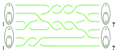
Figure 9: (color online). Two encoded qubits and a generic braid. Because quasiparticles are braided outside of their starting qubits these braids will generally lead to leakage out of the computational qubit space, i.e. the $q$-spin of each group of three quasiparticles forming these qubits will in general no longer be 1.

VI Two-qubit Gates

We have seen that single-qubit gates are “easy” in the sense that as long as we braid within an encoded qubit there will be no leakage errors (the overall $q$-spin of the group of three quasiparticles will remain 1). Furthermore, the space of unitary operators acting on the three-quasiparticle Hilbert space (essentially $SU(2)$) is small enough to find excellent approximate braids by performing brute force searches and subsequent improvement using the Solovay-Kitaev algorithm. We now turn to the significantly harder problem of finding braids which approximate entangling two-qubit gates.

VI.1 “Divide and Conquer” Approach

Figure 9 depicts six quasiparticles encoding two qubits and a general braiding pattern. To entangle these qubits, quasiparticles from one qubit must be braided around quasiparticles from the other qubit, and this will inevitably lead to leakage out of the encoded qubit space, (i.e. the overall $q$-spin of the three quasiparticles constituting a qubit may no longer be 1). Furthermore, the space of all operators acting on the Hilbert space of six quasiparticles is much bigger than for three, making brute force searching extremely difficult. Here the unitary operations acting on this space are in $SU(5)\oplus SU(8)$, (up to winding dependent phase factors as in (27)), which has 87 free parameters as opposed to 3 for the three quasiparticle case of $SU(2)$.

Still, as a matter of principle, it is possible to perform a brute force search of sufficient depth so that it corresponds to a fine enough $\epsilon$-net to carry out the Solovay-Kitaev algorithm in this larger space.kitaevbook This is essentially the program outlined in Ref. freedman1, as an “existence proof” that universal quantum computation is possible; however, it is not at all clear that, even if one could do this, it would be the most efficient procedure for compiling braids. For the same amount of classical computing power required to directly compile braids in $SU(5)\oplus SU(8)$, we believe one can find much more efficient (in the sense of having a more accurate computation with a shorter braid) braids by breaking the problem into smaller problems, each consisting of finding a specific three-braid embedded in the full six-braid space. As we’ve shown above, these three-braids can then be very efficiently compiled.

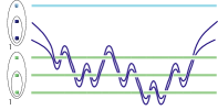
Figure 10: (color online). A two-qubit gate construction in which a pair of quasiparticles from the top (control) qubit is woven through the bottom (target) qubit. The mobile pair of quasiparticles is referred to as the control pair and has a total $q$-spin of 0 if the control qubit is in the state $|0_{L}\rangle$, and 1 if the control qubit is in the state $|1_{L}\rangle$. Since weaving an object with total $q$-spin 0 yields the identity operation, this construction is guaranteed to result in a transformation of the target qubit state only if the control qubit is in the state $|1_{L}\rangle$. Note that in this and subsequent figures world-lines of mobile quasiparticles will always be dark blue.

Here we present two classes of two-qubit gate constructions based on this “divide and conquer” approach. The first of these were originally introduced by the authors in Ref. bonesteel05, and are characterized by the weaving of a pair of quasiparticles from one qubit through the quasiparticles forming the second qubit. The second class, presented here for the first time, can be carried out by weaving only a single quasiparticle from one qubit around one other quasiparticle from the same qubit, and two quasiparticles from the second qubit.

VI.2 Two-Quasiparticle Weave Construction

We now review the two-qubit gate constructions first discussed in Ref. bonesteel05, . The basic idea behind these constructions is illustrated in Fig. 10. This figure shows two qubits and a braiding pattern in which a pair of quasiparticles from the top qubit (the control qubit) is woven through the quasiparticles forming the bottom qubit (the target qubit). Throughout this braiding the pair is treated as a single immutable object which, at the end of the braid, is returned to its original position.

If, as in Fig. 10, we choose the pair of weft quasiparticles to be the two quasiparticles whose total $q$-spin determines the logical state of the qubit, then we refer to this pair as the control pair. We can then immediately see why this construction naturally suggests itself. If the control qubit is in the state $|0_{L}\rangle$ the control pair will have total $q$-spin 0, and weaving this pair through the target qubit will have no effect. We are thus guaranteed that if the control qubit is in the state $|0_{L}\rangle$ the identity operation is performed on the target qubit.

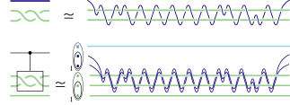
Figure 11: (color online). An effective braiding weave, and a two-qubit gate constructed using this weave. The effective braiding weave is a woven three-braid which produces a unitary operation which is a distance $\epsilon\simeq 2.3\times 10^{-3}$ from that produced by simply interchanging the two target particles ($\sigma_{1}^{2}$). When the control pair is woven through the target qubit using this weave the resulting two-qubit gate approximates a controlled-$(\sigma_{2}^{2})$ gate to a distance $\epsilon\simeq 1.9\times 10^{-3}$ or $\epsilon\simeq 1.6\times 10^{-3}$ when the total $q$-spin of the two qubits is 0 or 1, respectively.

The only non-trivial effect of this weaving pattern occurs when the control qubit is in the state $|1_{L}\rangle$. In this case, the control pair has total $q$-spin 1 and so behaves as a single Fibonacci anyon. The problem of constructing a two-qubit controlled gate then corresponds to finding a weaving pattern in which a single Fibonacci anyon weaves through the three quasiparticles of the target qubit, inducing a transition on this qubit without inducing leakage error out of the computational qubit space, or at least keeping such leakage as small as required for a particular computation. This reduces the problem of finding a two-qubit gate to that of finding a weaving pattern in which one Fibonacci anyon weaves around three others — a problem involving only four Fibonacci anyons. However, following our “divide and conquer” philosophy, we will further narrow our focus to weaving a single Fibonacci anyon through only two others at a time.

We define an “effective braiding” weave, to be a woven three-braid in which the weft quasiparticle starts at the top position, and returns to the top position at the end of the weave, with the requirement that the unitary transformation it generates be approximately equal to that produced by $m$ clockwise interchanges of the two warp quasiparticles. To find such weaves we perform a brute force search, as outlined in Sec. V, over sequences $\{n_{i}\}$ which approximately satisfy

$$\sigma_{2}\>U_{\rm weave}(\{n_{i}\})\>\sigma_{2}\simeq\sigma_{1}^{m}.$$ (33)

If both sides of this equation are expressed using (27) it becomes evident that the winding of any effective braiding weave must satisfy $W=m$ (modulo 10). Since the weft particle starts and ends in the top position, $W$ must be even, thus effective braiding weaves only exist for even $m$.

An example of an $m=2$ effective braiding weave found through a brute force search is shown in Fig. 11. The corresponding unitary operation approximates that of interchanging the two warp quasiparticles twice to a distance $\epsilon\sim 10^{-3}$. (This is a typical distance for a woven three-braid of length $L\simeq 46$ which approximates a desired operation — precise distances of approximate weaves are given in the figure captions.) As for all approximate weaves considered here, the Solovay-Kitaev algorithm outlined in Sec. V.C can be used to improve the accuracy of this weave so that $\epsilon$ can be made as small as required with only a polylogarithmic increase in length.

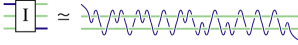
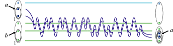
Figure 12: (color online). An injection weave, and step one in our injection based gate construction. The box labeled $I$ represents an ideal (infinite) injection weave which is approximated by the weave shown to a distance $\epsilon\simeq 1.5\times 10^{-3}$. In step one of our gate construction, this injection weave is used to weave the control pair into the target qubit. If the control qubit is in the state $|1_{L}\rangle$ then $a=1$ and the result is to produce a target qubit with the same quantum numbers as the original, but with its middle quasiparticle replaced by the control pair.

The construction of a two-qubit gate using this effective braiding weave is also shown in Fig. 11. In this construction the control pair is woven through the top two quasiparticles of the target qubit using this weave. As described above, if the control qubit is in the state $|0_{L}\rangle$, the control pair has $q$-spin 0 and the target qubit is unchanged. But, if the control qubit is in the state $|1_{L}\rangle$, the control pair has $q$-spin 1 and the action on the target qubit is approximately equivalent to that of interchanging the top two quasiparticles twice, with the approximation becoming more accurate as the length of the effective braiding weave is increased, either by deeper brute force searching or by applying the Solovay-Kitaev algorithm. Because this effective braiding all occurs within an encoded qubit, leakage errors can be reduced to zero in the limit $\epsilon\rightarrow 0$. The resulting two-qubit gate is then a controlled-$\sigma_{2}^{2}$ gate which corresponds to controlled rotation of the target qubit through an angle of $6\pi/5$.

Unfortunately, due to the even $m$ constraint, it is impossible to find an effective braiding gate which corresponds to a controlled $\pi$ rotation of the target qubit. Such a gate would be equivalent to a controlled-NOT gate up to single-qubit rotations.nielsenbook Nonetheless, it is known that any entangling two-qubit gate, when combined with the ability to carry out arbitrary single-qubit rotations, forms a universal set of quantum gates.notcnot Thus, the efficient compilation of single-qubit operations described in Sec. V and the effective braiding construction just given provide direct procedures for compiling any quantum algorithm into a braid to any desired accuracy.

Although it can be used to form a universal set of gates, this effective braiding construction is still rather restrictive. It is clearly desirable to be able to directly compile a controlled-NOT gate into a braid. We now give a construction which can be used to efficiently compile any arbitrary controlled rotation of the target qubit — including a controlled-NOT gate. This construction is based on a class of woven three-braids which we call “injection weaves”.

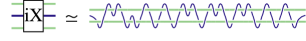
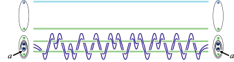
Figure 13: (color online). A weave which approximates $iX$ (see Eq. 32), and step two in our injection based construction. The box labeled $iX$ represents an ideal (infinite) $iX$ weave which is approximated by the weave shown to a distance $\epsilon=8.5\times 10^{-4}$ (this is the same weave which appears at the top of Fig. 8). In step two of our gate construction the control pair is woven within the injected target qubit, following this weave, in order to carry out an approximate $iX$ gate when $a=1$, as shown.

In an injection weave the weft quasiparticle again starts at the top position but in this case ends at a different position. At the same time we require that the unitary operation generated by this weave approximate the identity. Thus the effect of an injection weave is to permute the quasiparticles involved without changing any of the underlying $q$-spin quantum numbers of the system.

Comparing the identity matrix to (27) we see that any three-braid approximating the identity must have winding $W=0$ (modulo 10). The fact that this winding must be even implies that the final position of the weft particle must be at the bottom of the weave. Thus injection weaves correspond to sequences $\{n_{i}\}$ which approximately satisfy the equation,

$$\sigma_{1}\>U_{\rm weave}(\{n_{i}\})\>\sigma_{2}\simeq\left(\begin{array}[]{cc|c}1&0&\\ 0&1&\\ \hline\cr&&1\end{array}\right).$$ (37)

An injection weave obtained through brute force search is shown in Fig. 12. The unitary operation produced by this weave approximates the identity operation to a distance $\epsilon\sim 10^{-3}$.

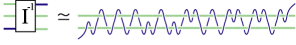
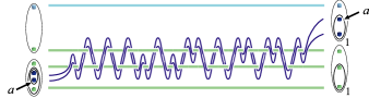
Figure 14: (color online). An inverse injection weave and step three in our injection based construction. The box labeled $I^{-1}$ represents an ideal (infinite) inverse injection weave which is approximated by the the inverse of the injection weave shown in Fig. 12, again to a distance $\epsilon\simeq 1.5\times 10^{-3}$. This weave is used to extract the control pair out of the injected target qubit and return it to the control qubit, as shown.

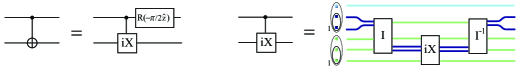
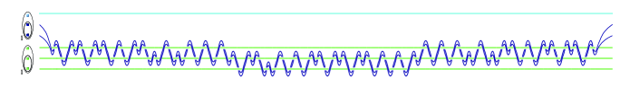
Figure 15: (color online). Injection-weave based compilation of a controlled-NOT gate into a braid. A controlled-NOT gate can be expressed as a controlled-$(iX)$ gate and a single-qubit operation $R(-\pi/2\ \hat{z})=\exp(i\pi\sigma_{z}/4)$ acting on the control qubit. The single-qubit rotation can be compiled following the procedure outlined in Sec. V, and the controlled-$(iX)$ gate can be decomposed into ideal injection ($I$), $iX$, and inverse injection ($I^{-1}$) operations which can be similarly compiled. The full approximate controlled-$(iX)$ braid obtained by replacing $I$, $iX$ and $I^{-1}$ with the weaves shown in the previous three figures is shown at bottom. The resulting gate approximates a controlled-$(iX)$ to a distance $\epsilon\simeq 1.8\times 10^{-3}$ and $\epsilon\simeq 1.2\times 10^{-3}$ when the total $q$-spin of the two qubits is 0 or 1, respectively.

Our two-qubit gate construction based on injection weaving is carried out in three steps. In the first step, also shown in Fig. 12, the control pair is woven into the target qubit using the injection weave. If the control pair has total $q$-spin 1 (the only nontrivial case) the effect of this weave is merely to replace the middle quasiparticle of the target qubit with the control pair. Because the unitary operation approximated by the injection weave is the identity, in the $\epsilon\rightarrow 0$ limit this injection is accomplished without changing any of the $q$-spin quantum numbers. The injected target qubit is therefore (approximately) in the same quantum state as the original target qubit.

In the second step of our construction, illustrated in Fig. 13, we carry out an operation on the injected target qubit by simply weaving the control pair within the target. Because for $a=1$ all of this weaving takes place within the injected target qubit, there will be no leakage error (again, strictly speaking, only in the limit of an exact injection weave). The only constraint on this weave is that the control pair must both start and end in the middle position, and so it must have even winding.

If our goal is to produce a gate which is equivalent to a controlled-NOT gate up to single-qubit rotations then we must apply a $\pi$ rotation to the target qubit. Unfortunately, this cannot be accomplished by any finite weave with even winding, so we must again consider approximate weaves. Figure 13 shows the control pair being woven through the injected target qubit using a weave found by a brute force search which approximates a particular $\pi$ rotation — the operator $iX$ defined in (32) — to a distance $\epsilon\sim 10^{-3}$ (this is, in fact, the same weave shown at the top of Fig. 8).

The third step in our construction is the extraction of the control pair from the target qubit. This is accomplished, as shown in Fig. 14, by applying the inverse of the injection weave to the control pair. The effect of this extraction is to restore the control qubit to its original state, and replace the control pair inside the target qubit with the quasiparticle which originally occupied that position.

The full construction is summarized in Fig. 15, which provides a recipe for compiling a controlled-NOT gate into a two-quasiparticle weave. A quantum circuit showing that a controlled-NOT gate is equivalent to a controlled-$(iX)$ gate and a single-qubit operation is shown in the top part of the figure. The single-qubit operation can be compiled to whatever accuracy is required following Sec. V, and the controlled-$(iX)$ gate can be decomposed into injection, $iX$, and inverse injection operations, as is also shown in the top part of the figure. These operations can then all be similarly compiled following Sec. V.

The full braid shown at the bottom of Fig. 15 corresponds to using the approximate woven three-braids shown in Figs. 12-14 to carry out a controlled-$(iX)$ gate. In this braid, if the control qubit is in the state $|0_{L}\rangle$ the control pair has total $q$-spin 0 and the resulting unitary transformation is exactly the identity. However, if the control qubit is in the state $|1_{L}\rangle$ the control pair has total $q$-spin 1 and behaves like a single Fibonacci anyon. This pair is then woven into the target qubit using an injection weave, woven within the target in order to carry out the $iX$ operation, and finally woven out of the target and back into the control qubit using the inverse of the injection weave. The resulting gate is therefore a controlled-$(iX)$ gate.

By replacing the $iX$ weave with an even winding weave which carries out an arbitrary operation $U$ this construction will give a controlled-$U$ gate. The only restriction on $U$ is that its overall phase must be consistent with (27) with even winding $W$. However, this phase can be easily set to any desired value by applying the appropriate single-qubit rotation to the control qubit, as in Fig. 15.

Finally, note that at no point in either the effective braiding or injection weave constructions described above did we make reference to the total $q$-spin of the two qubits involved. It follows that, in the limit of exact effective braiding or injection weaves, the action of the corresponding two-qubit gates on the computational qubit space does not depend on the state of the external fusion space associated with the $q$-spin 1 quantum numbers of each qubit (see Sec. IV). These gates will therefore not entangle the computational qubit space with this external fusion space.

VI.3 One-Quasiparticle Weave Constructions

We now show that two-qubit gates can be carried out with only a single mobile quasiparticle. This possibility follows from the general result of Ref. simon06, that for any system of nonabelian quasiparticles in which general braids are universal for quantum computation (such as Fibonacci anyons), single quasiparticle weaves are universal as well. However, the “proof of principle” weaves constructed in that work were extremely inefficient — involving a huge number of excess operations. Here we show how to efficiently construct a single-quasiparticle weave corresponding to a controlled-NOT gate (up to single-qubit rotations).

Our construction is based on a class of weaves which are similar to injection weaves in that they can be used to swap two $q$-spin 1 objects — where one object is a pair of Fibonacci anyons with total $q$-spin 1 and the other object is a single Fibonacci anyon — while acting effectively as the identity operation so that none of the other $q$-spin quantum numbers of the system are disturbed. However, unlike injection weaves, this new class of weaves accomplish this swap without moving the pair as a single object, and in fact can be carried out by moving just one quasiparticle.

The class of weaves we seek are those which approximate the transformation

$$U((\bullet,\bullet)_{a},\bullet)_{c}=e^{i\phi}(\bullet,(\bullet,\bullet)_{a})_{c},$$ (38)

where $\phi$ is an overall (irrelevant) phase which does not depend on $a$ or $c$. The relevant case for showing the similarity with injection is when $a=1$, for which the initial and final states in (38) consist of two $q$-spin 1 objects — a single Fibonacci anyon and a pair of Fibonacci anyons with total $q$-spin 1. If both these objects are represented as single Fibonacci anyons then (38) can be written $U(\bullet,\bullet)_{c}=e^{i\phi}(\bullet,\bullet)_{c}$. In this representation $U$ therefore acts effectively as the identity operation (times an irrelevant phase), similar to injection.

Using the $F$ matrix (8) to expand the right hand side of (38) in the $((\bullet,\bullet),\bullet)$ basis yields

$$U((\bullet,\bullet)_{a},\bullet)_{c}=e^{i\phi}\sum_{b}F^{c}_{ab}((\bullet,\bullet)_{b},\bullet)_{c}.$$ (39)

Comparing this with the action of a unitary operation $U$ with matrix representation

$$U=\left(\begin{array}[]{cc|c}U^{1}_{00}&U^{1}_{01}&\\ U^{1}_{10}&U^{1}_{11}&\\ \hline\cr&&U^{0}_{11}\end{array}\right),$$ (43)

on the state $((\bullet,\bullet)_{a},\bullet)_{c}$,

$$U((\bullet,\bullet)_{a},\bullet)_{c}=\sum_{b}U^{c}_{ab}((\bullet,\bullet)_{b},\bullet)_{c},$$ (44)

we see that the matrix representation of the $U$ we seek is precisely the $F$ matrix (up to a phase): $U=e^{i\phi}F$. While the $F$ matrix describes a “passive” operation, i.e. a change of basis, the operator $U$ can be viewed as an “active” $F$ operation which acts directly on the states of the Hilbert space. Note that, since $F=F^{-1}$, we also have

$$U(\bullet,(\bullet,\bullet)_{a})_{c}=e^{i\phi}((\bullet,\bullet)_{a},\bullet)_{c}.$$ (45)

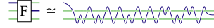
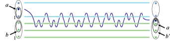
Figure 16: (color online). An $F$ weave, and step one of our $F$ weave based two-qubit gate construction. The box labeled $F$ represents an ideal (infinite) $F$ weave which is approximated by the weave shown to a distance $\epsilon\simeq 3.1\times 10^{-3}$. Applying the $F$ weave to the initial two-qubit state, as shown, produces an intermediate state with $q$-spins labeled $a$ and $b^{\prime}$ which depend simply on $a$ and $b$ — the initial states of the two qubits (see Table I).

We will refer to weaves which approximate the operation (38) (and thus also (45)) as $F$ weaves. As we have seen, the unitary operation $U$ produced by an $F$ weave need only approximate the $F$ matrix (8) up to an overall irrelevant phase. To be consistent with (27) this phase must be $-1$, as can be seen by writing the matrix $-F$ as

$$-F=\left(\begin{array}[]{c|c}\pm i\left(\begin{array}[]{cc}\pm i\tau&\pm i\sqrt{\tau}\\ \pm i\sqrt{\tau}&\mp i\tau\end{array}\right)\\ \hline\cr&-1\end{array}\right),$$ (50)

where a factor of $\pm i$ has been pulled out of the upper left 2$\times$2 block, leaving an $SU(2)$ matrix ($\det=\tau^{2}+\tau=1$). Comparing (50) with (27), it is also evident that any $F$ weave must have winding $W=$ 5 (modulo 10), which is necessarily odd.

The fact that $F$ weaves must have an odd number of windings implies that if the weft quasiparticle starts at the top position of the weave it must end at the middle position. For this choice the $F$ weave must then approximately satisfy the equation

$$U_{\rm weave}(\{n_{i}\})\>\sigma_{2}\simeq-F.$$ (51)

The result of a brute force search for an $F$ weave which approximates the operation $-F$ to a distance $\epsilon\sim 10^{-3}$ is shown in Fig. 16.

The first step in our single-quasparticle weave construction is the application of an $F$ weave to two qubits, also shown in Fig. 16. Note that in this figure for convenience we have made a change of basis on the bottom qubit, so that the pair which determines its state (the control pair) consists of the top two quasiparticles within it rather than the bottom two. There is no loss of generality in doing so since this just corresponds to a single-qubit rotation on the bottom qubit.

With this basis choice the initial state of the two qubits is determined by the $q$-spins of their respective control pairs which are indicated in Fig. 16 as $a$ (top qubit) and $b$ (bottom qubit). After carrying out the $F$ weave, taking the middle quasiparticle of the top qubit as the weft quasiparticle and weaving it around both the bottom quasiparticle of the top qubit and the top quasiparticle of the bottom qubit, the resulting state (again, strictly speaking, only in the limit of an exact $F$ weave) is shown at the end of the two-qubit weave in Fig. 16. From (45) it follows that the newly positioned weft quasiparticle and the quasiparticle beneath will have total $q$-spin $a$. When the quasiparticle beneath these two is also included, the three quasiparticles form what we will refer to as the intermediate state, $(\bullet,(\bullet,\bullet)_{a})_{b^{\prime}}$, where the total $q$-spin of all three quasiparticles, $b^{\prime}$, has a well-defined value provided $a$ and $b$ are well defined, as we now show.

$a$	$b$		$b^{\prime}$	Phase Factor
0	0	$b^{\prime}=1$	1	$e^{i\alpha}$
0	1		1	$e^{i\alpha}$
1	0	$b^{\prime}=b$	0	1
1	1		1	$e^{-i\alpha}$

Table 1: Values of $b^{\prime}$ for different values of $a$ and $b$ after applying the $F$ weave as shown in Fig. 16, and the phase applied to the resulting state by a phase weave with zero winding. The value of $b^{\prime}$ is determined by the fact that $b^{\prime}=1$ when $a=0$ and $b^{\prime}=b$ when $a=1$, as shown in the text.

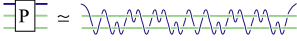
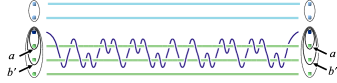
Figure 17: (color online). A phase weave with $\alpha=\pi$ (see text) which gives a $\pi$ phase shift to the intermediate state when $b^{\prime}=1$, and step two of our $F$ weave based construction. The box labeled $P$ represents an ideal (infinite) $\alpha=\pi$ phase weave which is approximated by the weave shown to a distance $\epsilon\simeq 1.9\times 10^{-3}$. Applying this phase weave to the intermediate state created by the $F$ weave, as shown, results in a $b^{\prime}$ dependent $\pi$ phase shift (see Table I with $\alpha=\pi$).

First consider the case $a=1$. As described above, the effect of the $F$ weave is then similar to that of the injection weave from the previous construction — it replaces the topmost quasiparticle in the bottom qubit with a pair of quasiparticles with $q$-spin 1, and the bottommost pair of quasiparticles in the top qubit (which also has total $q$-spin 1) with a single quasiparticle, without changing any of the other $q$-spin quantum numbers of the system. In the limit of an ideal $F$ weave, this means that the $b$ quantum number does not change after this swap and so $b^{\prime}=b$. The case $a=0$ is simpler, since in this case the intermediate state is $(\bullet,(\bullet,\bullet)_{0})_{b^{\prime}}$ for which the fusion rules (2) imply $b^{\prime}=1$, regardless of the value of $b$. The resulting dependence of $b^{\prime}$ on $a$ and $b$ is summarized in Table 1.

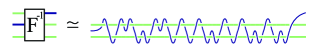
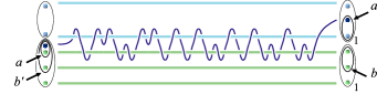
Figure 18: (color online). An inverse $F$ weave and step three in our $F$ weave construction. The box labeled $F^{-1}$ is an ideal (infinite) inverse $F$ weave which is approximated by the inverse of the $F$ weave shown in Fig. 16, again to a distance $\epsilon\simeq 3.1\times 10^{-3}$. By applying the inverse $F$ weave to the state obtained after applying the phase weave, as shown, the two qubits are returned to their initial states, but now with an $a$ and $b$ dependent phase factor (see Table I).

Having used the $F$ weave to create the intermediate state $(\bullet,(\bullet,\bullet)_{a})_{b^{\prime}}$, the next step in our construction is the application of a weave which performs an operation on this state which does not change $a$ and $b^{\prime}$ but which does yield an $a$ and $b^{\prime}$ dependent phase factor. After carrying out such a weave, which we will refer to as a phase weave, we can then apply the inverse of the $F$ weave to restore the two qubits to their initial states $a$ and $b$.

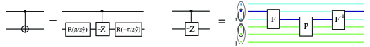
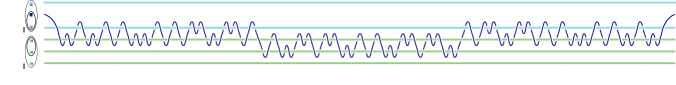
Figure 19: (color online). $F$ weave based compilation of a controlled-NOT gate into a braid. A controlled-NOT gate is equivalent to a controlled-$(-Z)$ gate with the single-qubit operation $R(\pi/2\ \hat{y})=\exp(-i\pi\sigma_{y}/4)$ and its inverse applied to the target qubit before and after the controlled-$(-Z)$. Again, the single-qubit operations can be trivially compiled, and the controlled-$(-Z)$ gate decomposed into ideal $F$, phase $(P)$, and inverse $F$ ($F^{-1}$) weaves which can be similarly compiled. The full approximate controlled-$(-Z)$ weave obtained by replacing $F$, $P$ and $F^{-1}$ with the approximate weaves shown in the previous three figures is shown at bottom. The resulting gate approximates a controlled-$(-Z)$ to a distance $\epsilon\simeq 4.9\times 10^{-3}$ and $\epsilon\simeq 3.2\times 10^{-3}$ when the total $q$-spin of the two qubits is 0 or 1, respectively.

For any phase weave we will require that the weft quasiparticle both start and end in the top position so that when we join it to the $F$ weave and its inverse there will be a single weft quasiparticle throughout the entire gate construction. The phase weave must therefore have even winding, and with no loss of generality we can consider the case for which the winding satisfies $W=0$ (modulo 10). The unitary operation produced by such a phase weave must then approximately satisfy the equation

$$\sigma_{2}U_{\rm weave}(\{n_{i}\})\sigma_{2}\simeq F\left(\begin{array}[]{cc|c}e^{i\alpha}&0&\\ 0&e^{-i\alpha}&\\ \hline\cr&&1\end{array}\right)F^{-1},$$ (55)

where the $F$ matrices are needed to change the Hilbert space basis from that in which the operation produced by the phase braid must be diagonal, (the $(\bullet,(\bullet,\bullet))$ basis), to that in which the $\sigma_{1}$ and $\sigma_{2}$ matrices are defined, (the $((\bullet,\bullet),\bullet)$ basis).

We will see that a phase weave with $\alpha=\pi$ produces a two-qubit gate which is equivalent to a controlled-NOT gate up to single-qubit rotations. The result of a brute force search for such a phase weave which approximates the desired operation to a distance $\epsilon\sim 10^{-3}$ is shown in Fig. 17. This figure also shows the action of the phase weave on the intermediate state produced in Fig. 16. In this weave, the weft quasiparticle is now woven through the two quasiparticles beneath it, and returns to its original position. Because the phase weave produces a diagonal operation in the basis shown for the intermediate state, it does not change the values of $a$ and $b^{\prime}$. Its only effect is to give a phase factor of $e^{i\alpha}$ to the state with $a=0$ (which necessarily has $b^{\prime}=1$) and $e^{-i\alpha}$ to the state with $a=1$ and $b^{\prime}=1$. The state with $a=1$ and $b^{\prime}=0$ is unchanged. These phase factors are also shown in Table 1.

The final step in this construction is to perform the inverse of the $F$ weave to return the two qubits to their original states. This is shown in Fig. 18. In the limit of exact $F$ and phase weaves, the resulting operation on the computational qubit space in the basis $ab=\{00,01,10,11\}$ is then,

$$U=\left(\begin{array}[]{cccc}e^{i\alpha}&0&0&0\\ 0&e^{i\alpha}&0&0\\ 0&0&1&0\\ 0&0&0&e^{-i\alpha}\end{array}\right).$$ (60)

If we take the top qubit to be the control qubit, and the bottom qubit to be the target qubit, then this gate corresponds, up to an irrelevant overall phase, to a controlled-($e^{-i3\alpha/2}e^{i\alpha\sigma_{z}/2})$ operation. For the case $\alpha=\pi$ this is a controlled-$(-Z)$ gate (where $Z=\sigma_{z}$), i.e. a controlled-Phase gate, which, up to single-qubit rotations, is equivalent to a controlled-NOT gate.

The full $F$ weave based gate construction is summarized in Fig. 19. A quantum circuit showing a controlled-NOT gate in terms of a controlled-$(-Z)$ gate and two single-qubit operations is shown in the top part of the figure. As in our injection based construction, the single-qubit operations can be compiled to whatever accuracy is required following the procedure outlined in Sec. V. The controlled-$(-Z)$ gate can then be decomposed into ideal $F$, phase, and inverse $F$ weaves as is also shown in the top part of the figure. Woven three-braids which approximate these operations can then be compiled to whatever accuracy is required, again following Sec. V. The full controlled-$(-Z)$ weave corresponding to using the approximate $F$ and phase weaves shown in Figs. 16-18 is shown in the bottom part of the figure.

Finally, in this construction, as for the constructions described in Sec. VI.B, we at no point made reference to the total $q$-spin of the two qubits involved. Thus, in the limit of exact $F$ and phase weaves, the action of the two-qubit gates constructed here will not entangle the computational qubit space with the external fusion space associated with the $q$-spin 1 quantum numbers of each qubit.

VII What’s special about $k=3$?

All of the gate constructions discussed in this paper exploit the fact that the braiding and fusion properties of a pair of Fibonacci anyons are either trivial if their total $q$-spin is 0, or equivalent to those of a single Fibonacci anyon if their total $q$-spin is 1. The fact that these are the only two possibilities is a special property of the Fibonacci anyon model, and hence also the $SU(2)_{3}$ model, given their effective equivalence. It is then natural to ask to what extent our constructions can be generalized to $SU(2)_{k}$ CSW theories for different values of the level parameter $k$.

Of course we know from the results of Freedman et al.freedman2 that the $SU(2)_{k}$ representations of the braid group are dense for $k=3$ and $k>4$. Thus, for example, braids which approximate controlled-NOT gates on encoded qubits exist and can, in principle, be found for all these $k$ values. However, we will show below that things are somewhat simpler for the case $k=3$. Specifically we will show that for $k=3$, and only $k=3$, it is possible to carry out two-qubit entangling gates by braiding only four quasiparticles, as, for example, in our effective braiding and $F$ weave constructions.

Consider a pair of $SU(2)_{k}$ four-quasiparticle qubits as shown in Fig. 20. Here each quasiparticle is assumed to have $q$-spin 1/2 and the total $q$-spin of each qubit is required to be 0. The state of a given qubit is then determined by the $q$-spin of either the topmost or bottommost pair of quasiparticles within it, where, from the $SU(2)_{k}$ fusion rules (1), the $q$-spin of each pair must be the same for the total $q$-spin of the qubit to be 0. Thus, in Fig. 20, the state of the top qubit is determined by the $q$-spin labeled $a$ and the state of the bottom qubit is determined by the $q$-spin labeled $b$, where, again from the fusion rules (1), $a$ and $b$ can be either 0 or 1.

If we are only allowed to braid the middle four quasiparticles, as shown in Fig. 20, then the total $q$-spin of the two topmost quasiparticles of the top qubit and the two bottommost quasiparticles of the bottom qubit will remain, respectively, $a$ and $b$. It follows that if the two qubits are to remain in their computational qubit spaces, the total $q$-spin of the two topmost and two bottommost quasiparticles that are being braided must also remain, respectively, $a$ and $b$. (If this were not the case, the fusion rules (1) would imply that the total $q$-spin of the four quasiparticles forming each qubit would no longer be 0). Thus, in order for there to be no leakage errors after braiding these four quasiparticles, the resulting operation must be diagonal in $a$ and $b$.

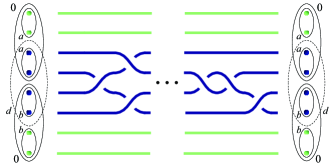
Figure 20: (color online). Two four-quasiparticle qubits and a braiding pattern in which only two quasiparticles from each qubit are braided. Here the quasiparticles are $SU(2)_{k}$ excitations with $q$-spin 1/2. The state of the top qubit is determined by the total $q$-spin of the quasiparticle pairs labeled $a$ and the state of the bottom qubit is determined by the total $q$-spin of the quasiparticle pairs labeled $b$. The overall $q$-spin of the four braided quasiparticles is $d$, (a dashed oval is used because when $a=b=1$ these quasiparticles will not be in a $q$-spin eigenstate). For this braid to produce no leakage errors, the unitary operation it generates must be diagonal in $a$ and $b$, though it can, of course, result in an $a$ and $b$ dependent phase factor. For $k>3$, $d$ can take the values 0, 1 or 2, while for $k=3$ the only allowed values for $d$ are 0 and 1. The existence of the $d=2$ state for $k>3$ makes it impossible to carry out an entangling two-qubit gate by braiding only four quasiparticles (see text).

It is important to note that this result, and the results that follow, hold not just for four-quasiparticle qubits, but also for $SU(2)_{k}$ versions of the three-quasiparticle qubits used throughout this paper. This is because, as pointed out in Sec. IV, any gate acting on a pair of three-quasiparticle qubits must result in an operation on the computational qubit space which is independent of the state of the external fusion space associated with the fact that each qubit has total $q$-spin 1/2, (here the total $q$-spin of a three-quasiparticle qubit is 1/2 rather than 1 because we are using $SU(2)_{k}$ quantum numbers and assuming each quasiparticle has $q$-spin 1/2 — see Fig. 3(b)). It is therefore sufficient to consider the special case when the state of two three-quasiparticle qubits corresponds to that of the two four-quasiparticle qubits shown in Fig. 20, but with the topmost and bottommost quasiparticles removed. The above arguments then imply any leakage free operation produced by braiding the four middle quasiparticles must be diagonal in $a$ and $b$.

Now consider the four middle quasiparticles we are allowed to braid. A basis for the Hilbert space of these quasiparticles can be taken to be one labeled by the $q$-spin quantum numbers $a$ and $b$, as well as the total $q$-spin of all four quasiparticles which we denote $d$ (see Fig. 20). For $k>3$ the fusion rules (1) imply this total $q$-spin $d$ can be equal to 0, 1 or 2, while for $k=3$ it can only be equal to 0 or 1. We will see that this truncation of the $d=2$ state is the crucial property of the $k=3$ theory which makes our $F$ weave and effective braiding constructions possible.

It is convenient at this stage to restrict ourselves to braids with zero total winding (i.e. equal numbers of clockwise and counterclockwise exchanges). For such braids, arguments similar to those used to derive (27) can be used to show the unitary operation enacted on the $d=0,1$ and 2 sectors must each have determinant 1. There is no loss of generality in restricting ourselves to such braids, since a braid with arbitrary winding can always be turned into one with zero winding by adding the appropriate number of interchanges to either the two topmost or two bottommost of the braiding quasiparticles at either the beginning or end of the braid. These added interchanges will all be within encoded qubits and so correspond to single-qubit rotations which will not produce any entanglement between the two qubits.

If we restrict ourselves to braids with zero winding and insist that these braids approximate gates with zero leakage error — which, as shown above, implies the gate must be diagonal in the $a$ and $b$ quantum numbers — then in the $abd=\{000,110,011,101,111,112\}$ basis the unitary transformation acting on the Hilbert space of the four braiding quasiparticles must have the form

$$U=\left(\begin{array}[]{cc|ccc|c}e^{i\alpha}&0&&&&\\ 0&e^{-i\alpha}&&&&\\ \hline\cr&&e^{i\beta}&0&0&\\ &&0&e^{i\gamma}&0&\\ &&0&0&e^{-i(\beta+\gamma)}&\\ \hline\cr&&&&&1\end{array}\right),$$ (67)

where we have required that the $d=0$, 1 and 2 blocks all have determinant 1, (in particular, the $d=2$ block is simply 1).

Note that the case $a=b=1$ has three entries in this matrix, corresponding to the three possible values for the total $q$-spin quantum number $d$. For this gate to produce no leakage error, the phase factors in all three of these sectors must be the same. To see this note that one can expand the relevant eight-quasiparticle state in terms of basis states with well-defined values of $d$ as follows

$$(((\bullet,\bullet)_{1},(\bullet,\bullet)_{1})_{0},((\bullet,\bullet)_{1},(\bullet,\bullet)_{1})_{0})_{0}$$

$$~{}=\sum_{d=0}^{2}F_{d}\ \left((\bullet,\bullet)_{1},\left((\bullet,\bullet)_{1},(\bullet,\bullet)_{1}\right)_{d},(\bullet,\bullet)_{1}\right)_{0},$$ (68)

where standard quantum group methodsslingerland01 ; fuchsbook can be used to compute the coefficients $F_{d}$, with the result

$$F_{0}=\frac{1}{[3]_{q}},\ \ F_{1}=\frac{\sqrt{[3]_{q}}}{[3]_{q}},\ \ F_{2}=\frac{\sqrt{[5]_{q}}}{[3]_{q}}.$$ (69)

Here we have introduced the $q$-integers $[m]_{q}\equiv(q^{m/2}-q^{-m/2})/(q^{1/2}-q^{-1/2})$, where $q=e^{i2\pi/(k+2)}$ is the deformation parameter.

For $k>3$ all three $F_{d}$ coefficients are nonzero. Thus, in order for the action of (67) on the $a=b=1$ state to produce the same state back (up to a phase), the projection of this state in the three $d$ sectors must all acquire the same phase. This implies that $\alpha=0$ and $\beta=-\gamma$. The resulting unitary operation must therefore take the form

$$U=\left(\begin{array}[]{cc|ccc|c}1&0&&&&\\ 0&1&&&&\\ \hline\cr&&e^{i\beta}&0&0&\\ &&0&e^{-i\beta}&0&\\ &&0&0&1&\\ \hline\cr&&&&&1\end{array}\right),$$ (76)

which corresponds to the following two-qubit gate in the $ab=\{00,01,10,11\}$ basis,

$$U^{gate}_{k>3}=\left(\begin{array}[]{cccc}1&0&0&0\\ 0&e^{i\beta}&0&0\\ 0&0&e^{-i\beta}&0\\ 0&0&0&1\end{array}\right).$$ (81)

This gate is simply the tensor product of two single-qubit rotations, $U^{gate}_{k>3}=e^{-i\beta\sigma_{z}^{(1)}/2}\otimes e^{i\beta\sigma_{z}^{(2)}/2}$. Thus we see that for $k>3$ any two-qubit gate constructed by braiding only four quasiparticles for which there is no leakage error must necessarily also produce no entanglement.

For $k=3$ this argument breaks down because the $d=2$ sector of the braiding quasiparticles is not present. In this case, following the same argument as above, in the $abd=\{000,110,011,101,111\}$ basis the allowed leakage free unitary transformations which can be produced by braiding the four middle quasiparticles must be of the form (again taking the case of zero winding),

$$U=\left(\begin{array}[]{cc|ccc}e^{i\alpha}&0&&&\\ 0&e^{-i\alpha}&&&\\ \hline\cr&&e^{i\beta}&0&0\\ &&0&e^{i(\alpha-\beta)}&0\\ &&0&0&e^{-i\alpha}\\ \end{array}\right),$$ (87)

which corresponds to the following two-qubit gate in the $ab=\{00,01,10,11\}$ basis,

$$U^{gate}_{k=3}=\left(\begin{array}[]{cccc}e^{i\alpha}&0&0&0\\ 0&e^{i\beta}&0&0\\ 0&0&e^{i(\alpha-\beta)}&0\\ 0&0&0&e^{-i\alpha}\end{array}\right).$$ (92)

As for $U_{k>3}^{gate}$, the $\beta$ dependence of $U_{k=3}^{gate}$ corresponds to a tensor product of single-qubit rotations. Gates of this form with fixed $\alpha$ but different values of $\beta$ are thus equivalent up to single-qubit rotations. If we use this equivalence to set $\beta=\alpha$ we see that gates of the form $U_{k=3}^{gate}$ are equivalent to the gates produced by our $F$ weave construction (60), and so, in particular, when $\alpha=\pi$ the resulting gate is equivalent to a controlled-NOT gate.

VIII Conclusions

To summarize, we have shown how to construct both single-qubit and two-qubit gates for qubits encoded using nonabelian quasiparticles described by $SU(2)_{3}$ CSW theory, or, equivalently, the $SO(3)_{3}$ theory (Fibonacci anyons). Qubits are encoded into triplets of quasiparticles and single-qubit gates are carried out by braiding quasiparticles within qubits. Two classes of two-qubit gate constructions were presented. In the first, a pair of quasiparticles from one qubit is woven through those forming the second qubit. In the second, a single quasiparticle is woven through three static quasiparticles (one from the same qubit as the mobile quasiparticle, the other two from the second qubit). A central theme in all of our two-qubit gate constructions is that of breaking the problem of compiling braids for the six quasiparticles used to encode two qubits into a series of braids involving only three objects at a time. While these constructions do not in general produce the optimal braid of a given length which approximates a desired two-qubit gate, we believe they do lead to the most accurate (or at least among the most accurate) two-qubit gates which can be obtained for a fixed amount of classical computing power. Finally, we proved a theorem which states that for the $SU(2)_{k}$ CSW theory, two-qubit gates constructed by braiding only four quasiparticles (two from each qubit) can only lead to leakage free entangling two-qubit gates when $k=3$.