Time-dependent Fröhlich transformation approach for
two-atom entanglement generated by successive passage through a cavity

Abstract

Time-dependent Fröhlich transformations can be used to derive an effective Hamiltonian for a class of quantum systems with time-dependent perturbations. We use such a transformation for a system with time-dependent atom-photon coupling induced by the classical motion of two atoms in an inhomogeneous electromagnetic field. We calculate the entanglement between the two atoms resulting from their motion through a cavity as a function of their initial position difference and velocity.

I Introduction

Canonical transformations have been widely used in condensed matter physics mah ; wagner to derive effective Hamiltonians by eliminating degrees of freedom with low-energy excitations zh . One of the most well-known applications was Fröhlich’s derivation fro of an attractive electron-electron interaction from the original electron-phonon interaction.

Fröhlich’s approach (which was also studied by Nakajima Naka ) was to apply a unitary transformation $H^{\prime}=\exp(-gS)H\exp(gS)$, defined by an anti-Hermitian operator $S$, to the Hamiltonian $H=H^{0}+gH^{1}$, where $H^{0}$ describes noninteracting electrons and phonons. His goal was to treat the electron-phonon interaction $gH^{1}$. The small parameter $g$ is introduced to stress that the interaction Hamiltonian is perturbative compared with the free Hamiltonian and can be set to $1$ during/after the calculation. The transformation can be evaluated order by order,

$$H^{\prime} =H^{0}+gH^{1}+g[H^{0},S]+g^{2}[H^{1},S]$$

$$+{\frac{g^{2}}{2}}[[H^{0},S],S]+O(g^{3}).$$ (1)

Fröhlich eliminated the term linear in $g$ by requiring

$$H^{1}+[H^{0},S]=0$$ (2)

to get the generator $S$. In the following, we will use the term Fröhlich transformation for a canonical transformation that fulfills Eq. (2). The transformation leads to a phonon-induced interaction among electrons with the potential $V=g^{2}\langle[H^{1},S]/2\rangle$ by averaging over the low-energy phonon states. This effective Hamiltonian can be attractive or repulsive with a singularity at the energy shell.

Since the interaction between atoms and electromagnetic field is similar to the electron-phonon coupling, it is natural to try to use Fröhlich transformations in quantum optics sun . In the large-detuning limit, i.e., if the difference between the atomic level spacing and the frequency of the light field is much larger than the coupling strength, the singularity at the energy shell is avoided, and the Fröhlich transformation is expected to work well. It will result in an effective Hamiltonian which can also be obtained from the adiabatic elimination method eberly90 and is equivalent to generic second-order perturbation theory.

However, in quantum optics and atomic physics, most realistic systems involve time-dependent classical fields. Obviously, a time-independent Fröhlich transformation cannot work for these cases. In this paper we use an effective Hamiltonian approach to eliminate certain intermediate degrees of freedom (e.g., the photon degree of freedom, or the atomic operators concerning a certain atomic level) corresponding to the time-dependent terms for the general case. A time-dependent transformation is used to make the first-order terms zero and to keep the second-order terms. We will call this method time-dependent Fröhlich transformation (TDFT).

The paper is organized as follows: in Section II we will briefly introduce the TDFT to fix the notation. In Section III and the following sections, we will use the TDFT approach to study the creation of two-atom entanglement after two atoms successively pass a cavity with a single mode field. As a result, we find that the entanglement depends on the atomic velocity (i.e., the transit time) and the initial distance between the two atoms. We determine the parameter regions for which the two atoms are maximally entangled, and discuss the limits of applicability of our method.

II Time-dependent canonical transformation

We consider a general time-dependent quantum system with a Hamiltonian

$$H=H^{0}+H^{1}(t),$$ (3)

where the unperturbed part $H^{0}$ is time-independent, and $H^{1}(t)$ is a time-dependent perturbation ($|H^{1}(t)|\ll|H^{0}|$). We perform the following time-dependent transformation:

$$\left|\psi^{\prime}(t)\right\rangle=e^{-S(t)}\left|\psi(t)\right\rangle,$$ (4)

where $|\psi(t)\rangle$ is a quantum state whose time dependence is governed by the Hamiltonian $H$. The transformed state $|\psi^{\prime}(t)\rangle$ evolves according to the unitarily transformed Hamiltonian

$$H^{\prime} =e^{-S}He^{S}+i\left(\partial_{t}e^{-S}\right)\cdot e^{S}$$

$$=H+\sum_{n=1}^{\infty}\frac{1}{n!}[...[H,S],...,S]$$

$$+i\partial_{t}\left(\sum_{n=0}^{\infty}\frac{(-S)^{n}}{n!}\right)\cdot\left(\sum_{n=0}^{\infty}\frac{S^{n}}{n!}\right).$$ (5)

Keeping the terms up to second order, we obtain the following effective Hamiltonian:

$$H_{\mathrm{eff}}^{\prime} =H^{0}+(H^{1}+[H^{0},S]-i\partial_{t}S)$$

$$+\frac{1}{2}[(H^{1}+[H^{0},S]-i\partial_{t}S),S]+\frac{1}{2}[H^{1},S].$$ (6)

If the operator $S(t)$ in the time-dependent transformation is chosen such as to make the first-order term of the effective Hamiltonian zero, that is

$$H^{1}+[H^{0},S]-i\partial_{t}S=0,$$ (7)

the effective Hamiltonian takes the simple form

$$H_{\mathrm{eff}}^{\prime}=H^{0}+\frac{1}{2}[H^{1},S].$$ (8)

The canonical transformation described by Eqs. (7) and (8) is the so-called time-dependent Fröhlich transformation (TDFT).

The form of the effective Hamiltonian after TDFT is similar to that in the time-independent case. Moreover, one also needs to have the formal solution for Eq. (7) to give an explicit expression for the effective Hamiltonian (8). We assume $\{|m\rangle$ $|m=0,1,2,...\}$ to be a set of eigenstates for the time-independent zeroth-order Hamiltonian $H^{0}$, and $E_{m}$ to be the eigenvalue for $\left|m\right\rangle$. The matrix elements of Eq. (7) in this basis lead to

$$H_{mn}^{1}+(E_{m}-E_{n})S_{mn}-i\partial_{t}S_{mn}=0,$$ (9)

where we have used the notation $(\partial_{t}S)_{mn}=\partial_{t}S_{mn}$ since $\left|m\right\rangle$ is time-independent. Thus, the solution for the transformation matrix elements $S_{mn}$ is given by note1

$$S(t)=-i\sum_{m,n}\int_{0}^{t}e^{-iE_{mn}(t-t^{\prime})}H_{mn}^{1}(t^{\prime})\mathrm{d}t^{\prime}\left|m\right\rangle\left\langle n\right|$$ (10)

with $E_{mn}:=E_{m}-E_{n}$ for any $m$ and $n$.

We would like to remark that TDFT is equivalent to second-order time-dependent perturbation theory (as proved in Appendix A). However, the effective Hamiltonian obtained after applying TDFT, Eq. (8), which contains only second-order interaction terms and no first-order interaction terms, is usually more convenient to be evaluated than the original Hamiltonian. For the time-independent weak-coupling atom-photon system (e.g., the systems given in Refs. sun ; Zheng and Guo , or the electron-phonon systems in Refs. zh ; Naka ), time-independent perturbation theory will give a second-order perturbation solution involving an infinite-dimensional Hilbert space. The equivalent conventional Fröhlich approach will give a decoupled effective Hamiltonian which can involve only the atomic part and can reduce to an analytically-solvable Hamiltonian in a finite-dimensional atomic Hilbert space. Similarly, in the time-dependent case, the interaction terms are time-dependent in the original Hamiltonian (3), and TDFT will give an effective (time-dependent) Hamiltonian, which may be decoupled from the photonic part and can be evaluated in the atomic Hilbert space. Therefore, applying TDFT can be much more efficient than using time-dependent perturbation theory.

In the following sections, we will give an example for the power of TDFT, namely, a system of two atoms that cross a single-mode optical cavity. This is by no means the only example. We expect that many atom-light or electron-phonon models that have been studied by the conventional Fröhlich approach (or other equivalent approaches) to eliminate certain degrees of freedom, are suitable to be evaluated by TDFT if the interaction depends on time. To conclude: TDFT is powerful for atom-light or electron-phonon models whose time-dependent interaction is perturbative.

III Time-dependent model for two atoms passing a cavity successively

We now use the TDFT method developed above to study a realistic physics problem in quantum optics. Entanglement is a defining feature of quantum mechanics that has no classical counterpart. It is an interesting issue to entangle two atoms separated by a large distance that have no direct interaction. Numerous proposals have been made for entangling atoms trapped in a cavity/cavities atom-cav01 ; atom-cav02 ; atom-cav03 ; Zheng and Guo ; Haroche01 ; HarocheRMP ; Haroche02 ; atom-cav04 ; atom-cav05 ; Walther05 ; Walther06 . Here, we will propose a scheme to entangle two identical two-level atoms, which are not trapped in a cavity but pass the single-mode optical cavity sequentially in transverse direction, see Fig. 1. Our goal is to calculate the degree of entanglement between these two atoms after this process. The coupling of the atoms to the cavity field is position-dependent, and their motion therefore causes a time-dependent coupling. If the coupling energy is assumed to be much less than the detuning between the atomic transition frequency and the optical frequency, that is, the large-detuning condition is satisfied, we can use the TDFT to get an effective time-dependent Hamiltonian, which only involves atom-atom interaction terms and eliminates the optical field.

A similar idea to entangle two atoms crossing a far-off-resonant single-mode cavity has been studied Zheng and Guo . However, there are significant differences between Ref. Zheng and Guo and our model: (i) In the proposal Zheng and Guo , both two-level atoms enter (or leave) the cavity with the same velocity at the same time. In our model, the two atoms have different initial positions, i.e., they enter the cavity with the same velocity at different times. In fact, we will study the degree of entanglement between the atoms as a function of the difference in initial position. (ii) In Ref. Zheng and Guo , the coupling between the atoms and the cavity is assumed to be constant. Therefore, it is possible to obtain an effective Hamiltonian with a reduced atom-atom interaction (assuming large detuning) by eliminating the photons (i.e., by means of the conventional Fröhlich transformation or other equivalent approaches). In reality, the coupling depends on the position the atom and has a Gaussian shape. Thus, the coupling is time-dependent when the atoms cross the cavity, and this is our motivation to use TDFT to study the present model. There are many other works on the generation of entanglement between two atoms crossing a cavity. Reference HarocheRMP describes experiments that study entanglement between two atoms after crossing a resonant-coupling cavity one by one. A two-qubit Grover quantum search algorithm is studied in Ref. Haroche02 by looking at two atoms crossing a large-detuning cavity (this model is similar to that in Ref. Zheng and Guo ). The generation and purification of maximally entangled states of two $\Lambda$-type-atoms inside a large-detuning cavity have also been investigated Walther05 . The important difference between all of the above models and our model is that the atom-photon coupling in the cavity is assumed to be constant in these models but is time-dependent in our model.

As can be seen from Fig. 1, the atoms are assumed to have the same constant velocity $v$ along the $z$-direction with both the initial positions $z_{1}^{0}$ and $z_{2}^{0}$ far away from the cavity. The Hamiltonian reads ($\hbar=1$)

$$H_{ori} =\omega_{0}(\sigma_{1}^{z}+\sigma_{2}^{z})+\omega a^{{\dagger}}a$$

$$+g_{1}(t)\sigma_{1}^{+}a+g_{2}(t)\sigma_{2}^{+}a+h.c.,$$ (11)

where $\sigma_{j}^{+}=\left|e\left\rangle{}_{jj}\right\langle g\right|$ and $\sigma_{j}^{z}=\left|e\left\rangle{}_{jj}\right\langle e\right|$ with $\left|e\right\rangle$ and $\left|g\right\rangle$ the atomic excited and ground states; $g_{j}(t)=g(z_{j}^{0}+vt)\sin(kx)$ are the coupling constants which are assumed to be of Gaussian form, $g(z)=g_{0}\exp(-z^{2}/d^{2})$, where $2d$ is the width of the cavity and $g_{0}$ the vacuum Rabi frequency. Here we set $\sin(kx)=1$ since the atoms are assumed to pass the cavity in transverse direction at a maximum of the standing light wave. It is also assumed that the atomic velocity along the $x$- and $y$-direction is zero. We ignore the back-action of the cavity to the momentum of the atoms since we assume the velocity to be large, (e.g., $v\sim 10$ m/s), such that the atomic decay time is long compared with the atomic cavity transit time. We assume the condition of large detuning is also fulfilled, $|\Delta|\gg|g_{0}|\gtrsim|g_{1,2}(t)|$ with the detuning $\Delta=\omega_{0}-\omega$, where $\omega_{0}$ ($\omega$) is the atomic transition frequency (optical frequency).

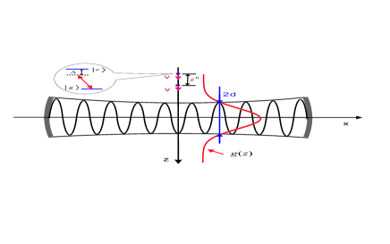
Figure 1: (Color online) Two atoms crossing the optical cavity. The width of the cavity is $2d$ and determines the profile of the coupling constant $g(z)=g_{0}\exp(-z^{2}/d^{2})$.

In the interaction picture with respect to

$$H_{ori}^{0}=\omega(\sigma_{1}^{z}+\sigma_{2}^{z})+\omega a^{{\dagger}}a,$$ (12)

the Hamiltonian (11) reads $H=H_{0}+H_{1}(t)$ where

$$H_{0} =\Delta(\sigma_{1}^{z}+\sigma_{2}^{z}),$$

$$H_{1} =g_{1}(t)\sigma_{1}^{+}a+g_{2}(t)\sigma_{2}^{+}a+h.c..$$ (13)

For large detuning, we can use a time-dependent Fröhlich transformation defined by

$$S(t)=x_{1}(t)\sigma_{1}^{+}a+x_{2}(t)\sigma_{2}^{+}a-h.c.$$ (14)

to eliminate the photon operators. The coefficients $x_{1,2}(t)$ satisfy the following equations:

$$g_{j}(t)+\Delta x_{j}(t)-i\dot{x}_{j}(t)=0,\ \ \ (j=1,2)$$ (15)

according to Eq. (7). The explicit solution for the coefficients $x_{1,2}(t)$ is given by note2

$$x_{j}(t)=-i\int_{0}^{t}g_{j}(t^{\prime})e^{i\Delta(t^{\prime}-t)}\mathrm{d}t^{\prime},\ \ \ (j=1,2).$$ (16)

After the Fröhlich transformation, the effective Hamiltonian reads (up to a constant term)

$$H_{\mathrm{eff}}^{\prime}(t) =H_{0}+\frac{1}{2}[H_{1}(t),S(t)]$$

$$=\Delta_{1}\sigma_{1}^{z}+\Delta_{2}\sigma_{2}^{z}+f\sigma_{1}^{-}\sigma_{2}^{+}+f^{\ast}\sigma_{1}^{+}\sigma_{2}^{-},$$ (17)

where

$$\Delta_{j}=\Delta-(g_{j}^{\ast}x_{j}+g_{j}x_{j}^{\ast})(1+2n_{p})$$ (18)

for $j=1,2$, $n_{p}=\langle a^{{\dagger}}a\rangle$ is the mean photon number in the cavity, and

$$f(t)=-\frac{1}{2}(g_{1}^{\ast}x_{2}+g_{2}x_{1}^{\ast})$$ (19)

is the effective coupling between the two atoms. The (first-order) weak interaction terms between the photons and atoms have been eliminated, and only the induced (second-order) atom-atom interaction terms remain. The Hamiltonian (17), which contains no photon operators (except the time-independent expectation value of the photon number operator), is much simpler than the original one (11). It can be diagonalized in the atomic basis

$$\{|g_{1}g_{2}\rangle,|g_{1}e_{2}\rangle,|e_{1}g_{2}\rangle,|e_{1}e_{2}\rangle\}\equiv\{|gg\rangle,|ge\rangle,|eg\rangle,|ee\rangle\}.$$ (20)

So far, we do not need any condition except the large detuning to get the simple effective Hamiltonian (17). In the following section, we will further simplify the effective Hamiltonian (17) using typical parameters for the cavity-QED system. As we will see below, the adiabatic condition is satisfied since the time-dependent couplings $g_{1,2}(t)$ are slowly varying (that is, $|\dot{g}_{j}(t)/g_{j}(t)|$ $\ll$ $|\Delta|$ for $j=1,2$). Of course, if the adiabatic condition is satisfied, the result obtained by TDFT in the next section can also be obtained by using adiabatic elimination. However, the elimination approach cannot be expected to describe our model if the adiabatic condition is not fulfilled.

IV Dynamical generation of two-atom entanglement

In the following, we will simplify the Hamiltonian (17) further by taking into account typical parameters for the cavity-QED system.

First, we will rewrite the coefficients (16) as follows:

$$x_{j}(t) \simeq-ie^{-i\Delta t}\int_{-\infty}^{t}g_{j}(t^{\prime})e^{i\Delta t^{\prime}}\mathrm{d}t^{\prime}$$

$$\simeq\frac{-e^{-i\Delta t}}{\Delta}\left\{g_{j}(t)e^{i\Delta t}+\frac{2v}{d}\int_{-\infty}^{t}g_{j}(t^{\prime})e^{i\Delta t^{\prime}}\mathrm{d}t^{\prime}\right\}$$

$$=-\frac{g_{j}(t)}{\Delta}-\frac{2iv}{\Delta d}x_{j}(t).$$ (21)

Here, we have used the explicit Gaussian form of the coupling constants. We have also used

$$\int_{-\infty}^{t}(z_{j}^{0}+vt)g_{j}(t^{\prime})e^{i\Delta t^{\prime}}\mathrm{d}t^{\prime}\rightarrow d\int_{-\infty}^{t}g_{j}(t^{\prime})e^{i\Delta t^{\prime}}\mathrm{d}t^{\prime}$$ (22)

since $z_{j}^{0}+vt\sim d$ in the effective integration range and the change of $g_{j}(t)$ (also change of $z_{j}^{0}+vt$) is much slower than that of $e^{i\Delta t}$:

$$F(g_{j}(t))\sim F(z_{j}^{0}+vt)\sim\frac{v}{d},\text{ }F(e^{-i\Delta t})\sim\Delta,$$ (23)

where $F(x):=\partial_{t}x/x\$denotes the change of $x$. For typical system parameters kimble ; blais ; you (wavelength of the atomic transition $\lambda=1000$ nm, detuning $\Delta=10^{4}$ MHz, $g_{0}=100$ MHz, cavity width (in the $z$-direction) $d=30\lambda$, and atomic velocity of the order of $v=10$ m/s), $(v/d)$ $\sim$ $10^{-1}$ MHz $\ll|\Delta|=10^{4}$ MHz, that is, the atomic cavity transit time $t_{transit}=2d/v$ is much larger than the time $1/\Delta$ according to the detuning. Actually, the fact that $v/d\ll|\Delta|$ (that is, $|\dot{g}_{j}(t)/g_{j}(t)|$ $\ll$ $|\Delta|$ for $j=1,2$) means the adiabatic condition is satisfied.

Using these parameter values, $x_{j}(t)$ in Eq. (21) can be further simplified as

$$x_{j}(t)\simeq-\frac{g_{j}(t)}{\Delta}-10^{-5}ix_{j}(t)\simeq-\frac{g_{j}(t)}{\Delta}=x_{j}^{\ast}(t).$$

The coefficients in Eq. (17) thus take the following form:

$$\Delta_{j}=\Delta+\frac{2(1+2n_{p})g_{j}^{2}(t)}{\Delta},$$ (24)

and the effective coupling is

$$f(t)=\frac{g_{1}(t)g_{2}(t)}{\Delta}.$$ (25)

We will now further assume that the shift terms in $\Delta_{j}$ can be ignored since $2g_{j}^{2}(t)/|\Delta|\ll|\Delta|$, i.e., we will replace the coefficients $\Delta_{j}$ by $\Delta$. Hence,

$$H_{\mathrm{eff}}^{\prime}(t)=\Delta\sigma_{1}^{z}+\Delta\sigma_{2}^{z}+f\sigma_{1}^{-}\sigma_{2}^{+}+f\sigma_{1}^{+}\sigma_{2}^{-}.$$ (26)

We now apply the transformation $U(t)=\exp\{(\Delta\sigma_{1}^{z}+\Delta\sigma_{2}^{z})t\}$ to the Hamiltonian $H_{\mathrm{eff}}^{\prime}(t)$ defined in Eq. (26) and obtain

$$H_{\mathrm{eff}}^{\prime\prime}(t)=f\sigma_{1}^{-}\sigma_{2}^{+}+f\sigma_{1}^{+}\sigma_{2}^{-}.$$ (27)

The time evolution of a general state governed by $H_{\mathrm{eff}}^{\prime\prime}(t)$ is given as

$$\left|\psi(t)\right\rangle=C_{gg}(t)\left|gg\right\rangle+C_{ge}(t)\left|ge\right\rangle+C_{eg}(t)\left|eg\right\rangle+C_{ee}(t)\left|ee\right\rangle,$$ (28)

where $C_{gg}(t)\equiv C_{gg}(0)$, $C_{ee}(t)\equiv C_{ee}(0)$, and

$$C_{ge}(t) =C_{ge}(0)\cos\theta(t)-iC_{eg}(0)\sin\theta(t),$$ (29)

$$C_{eg}(t) =-iC_{ge}(0)\sin\theta(t)+C_{eg}(0)\cos\theta(t),$$ (30)

with $\theta(t)=\int_{0}^{t}f(t^{\prime})\mathrm{d}t^{\prime}\simeq\int_{-\infty}^{t}f(t^{\prime})\mathrm{d}t^{\prime}$. Hence, the system described by Eq. (27) is characterized by a closed subspace $\{|ge\rangle,|eg\rangle\}$.

In what follows, we will investigate what degree of entanglement can be obtained after both atoms pass the cavity in transverse direction. We assume that the two atoms are prepared in the initial state $|\psi(0)\rangle=|ge\rangle$. The time evolution generated by Eq. (27) leads to

$$|\psi(t)\rangle=\cos\theta(t)|ge\rangle-i\sin\theta(t)|eg\rangle.$$ (31)

After both atoms have passed through the cavity and are far outside, that is $t\rightarrow+\infty$, one has

$$\theta(+\infty)=\sqrt{\frac{\pi}{2}}\frac{g_{0}^{2}d}{v\Delta}\mathrm{\exp}\left[-\frac{(z^{0})^{2}}{2d^{2}}\right],$$ (32)

where $z^{0}=z_{1}^{0}-z_{2}^{0}$ denotes the difference between the initial atomic positions.

In general, the state shown in Eq. (31) corresponds to an entangled state of the two atoms. In the following, we will study the degree of entanglement as a function of $z^{0}$ and the atomic velocity $v$ using the entanglement entropy that is defined as

$$E(\left|\psi(t)\right\rangle)=-\mathrm{Tr}(\rho_{1}\log_{2}\rho_{1}(t)).$$ (33)

Here, $|\psi(t)\rangle$ is a pure state, and $\rho_{1}(t)=\mathrm{Tr}_{2}(\left|\psi(t)\right\rangle\left\langle\psi(t)\right|)$ is the reduced density matrix of the first atom. Evaluating this expression for the state shown in Eq. (31), we obtain

$$E(\left|\psi(+\infty)\right\rangle) =-\cos^{2}\left[\theta(+\infty)\right]\log_{2}\cos^{2}\left[\theta(+\infty)\right]$$

$$-\sin^{2}\left[\theta(+\infty)\right]\log_{2}\sin^{2}\left[\theta(+\infty)\right].$$ (34)

A maximally entangled state for the atoms occurs for $\theta(+\infty)=(2n+1)\pi/4$ for any integer $n$. Figure 2 shows the entanglement entropy $E(|\psi(+\infty)\rangle)$ as a function of initial atomic position difference $z^{0}$ (in units of $d$) and atomic velocity $v$ (in units of $g_{0}^{2}d/\Delta$, which is 30 m/s for the system parameters discussed after Eq. (23)). The possible values for $z^{0}$ and $v$ which make the entanglement maximal (that is, $E(|\psi(+\infty)\rangle)=1$) are shown in Fig. 3.

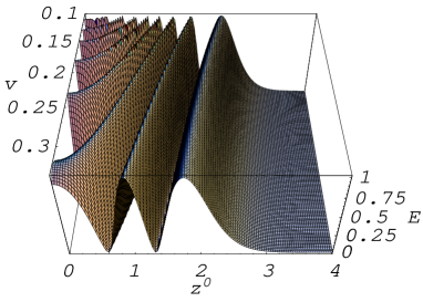
Figure 2: (Color online) Entanglement entropy $E$ as a function of atomic velocity $v$ (in units of $g_{0}^{2}d/\Delta$) and initial atomic position difference $z^{0}$ (in units of $d$).

It is interesting that there may be maximally entangled states for the two atoms even if the first atom has left the cavity before the second atom begins to enter it. For example, when the velocity $v$ is smaller than about $0.23g_{0}^{2}d/\Delta$ (corresponding to about $7$ m/s for the system parameters discussed after Eq. (23)), it is possible to obtain a maximally entangled state although the initial atomic position difference $z^{0}$ can be larger than $2d$ (i.e., the approximate transverse width of cavity), see Fig.3.

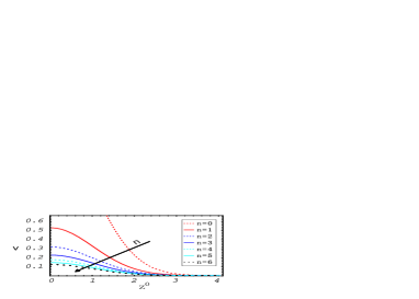
Figure 3: (Color online) Relation between atomic velocity $v$ (in units of $g_{0}^{2}d/\Delta$) and initial atomic position difference $z^{0}$ (in units of $d$) along the lines of maximal entanglement $E(+\infty)=1$, or $\theta(+\infty)=(2n+1)\pi/4$, for $n=0,1,...,6$.

In the above calculation, we have ignored the effect of (photonic and atomic) decay and photonic back-action to the atoms for the following reasons: (i) we assume that the velocity is of the order of $10$ m/s. Higher velocities will lead to a reduced degree of entanglement; lower velocities will lead to optical back-action to the atoms and photonic/atomic decay. (ii) we have assumed large detuning to reduce the atomic decay. (iii) the mean number of photons $n_{p}$ is assumed to be small (e.g. $10^{-4}$) in order to reduce the effect due to photonic decay. For example, the atomic cavity transit time (which is close to the interaction time) is less than the effective photonic decoherence time: $2d/v\sim 10^{-5}$ s $<1/(n_{p}\kappa)\sim 10^{-4}$ s (where $\kappa\sim 10^{8}$ Hz is the typical cavity one-photon damping rate blais ). Also, we have chosen $\Delta_{1,2}(t)$ $\rightarrow$ $\Delta$ which amounts to ignoring the effect of the shift terms in Eq. (24). The explicit form of $\Delta_{1,2}(t)$ shows that if the initial atomic position difference $z^{0}$ is close to $0$, then $\Delta_{1}(t)\rightarrow\Delta_{2}(t)$, and the effect of the shift terms can be neglected.

Finally, we would like to remark that the time-dependent Fröhlich transformation is valid under the condition of weak coupling (which is equivalent to the condition of large detuning here): $H_{1}(t)\ll H_{0}$ ($g_{0}\ll\Delta$). The adiabatic condition that the atomic cavity transit time $t_{transit}=2d/v$ is much larger than $1/\Delta$, is only used to simplify the effective coupling in Eq. (17) for the present realistic atoms-cavity system. Actually, this adiabatic condition is independent of the above large detuning condition for the time-dependent Fröhlich transformation. The above argument proves that, the TDFT approach is valid independent of whether the adiabatic condition is fulfilled or not.

V Conclusion

Using the time-dependent Fröhlich transformation, we have calculated the degree of atomic entanglement between two atoms passing an optical cavity sequentially. The Fröhlich transformation eliminates the photonic operators and induces an effective atom-atom interaction. We have determined the velocities and initial atomic position differences for which the entanglement is maximal, and we have shown that there may be maximally entangled states for the two atoms even if the first atom has left the cavity before the second atom begins to enter it.

A number of time-dependent canonical transformation methods have been proposed wagner ; wang to discuss time-dependent problems. The difference of our approach to a general time-dependent canonical transformation is that our TDFT requires the generator $S(t)$ in the canonical transformation to satisfy Eq. (7) in order to eliminate some intermediate degree of freedom for a general system. As an example, we have studied a system of two atoms that pass a cavity, which can be described by an effective atom-atom interaction Hamiltonian by using the TDFT to eliminate the photon degrees of freedom. In fact, the TDFT can be used to treat certain time-dependent atom-light systems by eliminating some of the atomic degree of freedom (e.g., one atomic level) like the Fröhlich transformation for the time-independent cases. The TDFT presented here works well not only for optical and atomic systems, but also in the field of condensed matter physics (e.g., time-dependent electron-phonon interactions) or other systems with weak (first-order) time-dependent interactions.

This work was supported by the European Union under contract IST-3-015708-IP EuroSQIP, by the Swiss NSF, and the NCCR Nanoscience. It was also supported by the NSFC with grant Nos. 90203018, 10574133, 10474104 and 60433050, and NFRPC with No. 2005CB724508.

Appendix A Equivalence to time-dependent second-order perturbation theory

To check the range of validity of the above effective Hamiltonian obtained by TDFT, we compare with the results of standard time-dependent perturbation theory up to of second order.

To apply time-dependent second-order perturbation theory for the Hamiltonian $H=H^{0}+H^{1}(t)$ given in Eq. (3), we assume $\{|m\rangle$ $|m=0,1,2...\}$ to be a complete set of eigenstates for the time-independent zeroth-order Hamiltonian $H^{0}$, with eigenvalues $E_{m}$. A state $|\psi(t)\rangle$ satisfies the Schrödinger equation

$$i\partial_{t}\left|\psi(t)\right\rangle=[H^{0}+H^{1}(t)]\left|\psi(t)\right\rangle.$$ (35)

We now do perturbation theory in $H^{1}(t)$ by assuming

$$\left|\psi(t)\right\rangle\equiv\sum_{l=0}\left|\psi^{(l)}(t)\right\rangle=\sum_{n=0,l=0}C_{n}^{(l)}(t)e^{-iE_{n}t}\left|n\right\rangle.$$ (36)

Here, $|\psi^{(l)}(t)\rangle$ is the $l$-order contribution to the perturbation expansion. Replacing $\left|\psi(t)\right\rangle$ in Eq. (35) by the perturbation expansion and comparing the coefficients order by order, we obtain the following equation:

$$i\dot{C}_{m}^{(l+1)}(t)=\sum_{n}C_{n}^{(l)}(t)e^{iE_{mn}t}H_{mn}^{1}(t).$$ (37)

If the initial state is $\left|k\right\rangle$, the zeroth-order solution for the coefficients $C_{n}(t)$ is

$$C_{m}^{(0)}(t)=\delta_{mk}.$$ (38)

According to Eq. (37) the first-order solution is

$$C_{m}^{(1)}(t)=-i\int_{0}^{t}e^{iE_{mk}t^{\prime}}H_{mk}^{1}(t^{\prime})\mathrm{d}t^{\prime}.$$ (39)

The second-order solution is

$$C_{m}^{(2)}(t)=-\sum_{n}\int_{0}^{t}\mathrm{d}t^{\prime}e^{iE_{mn}t^{\prime}}H_{mn}^{1}(t^{\prime})\int_{0}^{t^{\prime}}\mathrm{d}t^{\prime\prime}e^{iE_{nk}t^{\prime\prime}}H_{nk}^{1}(t^{\prime\prime}).$$ (40)

We will now consider the time evolution of the state predicted by the TDFT method. It follows from the Schrödinger equation

$$i\partial_{t}\left|\psi^{\prime}(t)\right\rangle=(H^{0}+\frac{1}{2}[H^{1},S])\left|\psi^{\prime}(t)\right\rangle$$ (41)

governed by the effective Hamiltonian $H_{\mathrm{eff}}^{\prime}$ in (8) after applying the TDFT method to the original Hamiltonian $H=H^{0}+H^{1}(t)$.

The connection to the original picture before the TDFT, i.e., the state $\left|\psi(t)\right\rangle$, whose time dependence is governed by $H$, reads

$$\left|\psi(t)\right\rangle\equiv(1+S+\frac{1}{2}S^{2}+...)|\psi^{\prime}(t)\rangle.$$ (42)

Like in Eq. (36), we can write down the perturbation expansion for $\psi^{\prime}(t)$:

$$\left|\psi^{\prime}(t)\right\rangle \equiv\sum_{l=0}|\psi^{\prime(l)}(t)\rangle=\sum_{n=0,l=0}C_{n}^{\prime(l)}(t)e^{-iE_{n}t}|n\rangle.$$ (43)

Starting with the initial state $\left|k\right\rangle$, and keeping terms up to the zeroth-order in Eq. (42), it is obvious that

$$|\psi^{(0)}(t)\rangle=|\psi^{\prime(0)}(t)\rangle,$$ (44)

and

$$C_{m}^{(0)}(t)=C_{m}^{\prime(0)}(t)=\delta_{mk}.$$ (45)

Since the perturbation term in $H_{\mathrm{eff}}^{\prime}$ is of second order, the first-order correction for $\left|\psi^{\prime}(t)\right\rangle$ vanishes: $\left|\psi^{\prime(1)}(t)\right\rangle=0$. Then from Eq. (42), the first-order correction for the state $|\psi(t)\rangle$ is

$$\left|\psi^{(1)}(t)\right\rangle=S\left|\psi^{\prime(0)}(t)\right\rangle.$$ (46)

Correspondingly, the first-order correction coefficients are

$$C_{m}^{(1)}(t)=-i\int_{0}^{t}e^{iE_{mk}t^{\prime}}H_{mk}^{1}(t^{\prime})\mathrm{d}t^{\prime}.$$ (47)

The results of Eq. (47) are equivalent to the standard time-dependent perturbation theory as shown in Eq. (39).

The second-order correction for $\left|\psi(t)\right\rangle$ is

$$\left|\psi^{(2)}(t)\right\rangle=\left|\psi^{\prime(2)}(t)\right\rangle+\frac{1}{2}S^{2}|\psi^{\prime(0)}(t)\rangle,$$ (48)

where $|\psi^{\prime(2)}(t)\rangle$ is the correction according to $[H^{1},S]/2$ in $H_{\mathrm{eff}}^{\prime}$ (8) with the exact form being given as (according to Eq. (39))

$$\left|\psi^{\prime(2)}(t)\right\rangle=\sum_{m}C_{m}^{\prime(2)}(t)e^{-iE_{m}t}\left|m\right\rangle$$ (49)

with

$$C_{m}^{\prime(2)}(t)=-\frac{i}{2}\int_{0}^{t}e^{iE_{mk}t^{\prime}}[H^{1}(t^{\prime}),S(t^{\prime})]_{mk}\mathrm{d}t^{\prime}.$$

Then the coefficients for the second-order corrections of the state $\left|\psi^{(2)}(t)\right\rangle$ are given as

$$C_{m}^{(2)}(t)=C_{m}^{\prime(2)}(t)+\frac{1}{2}\sum_{n}S_{mn}S_{nk}.$$

By replacing the operator $S(t)$ by that in Eq. (10) in the above equation, we obtain

$$C_{m}^{(2)}(t) = -\sum_{n}\int_{0}^{t}\mathrm{d}t^{\prime}e^{iE_{mn}t^{\prime}}H_{mn}^{1}(t^{\prime})$$ (50)

$$\times\int_{0}^{t^{\prime}}\mathrm{d}t^{\prime\prime}e^{iE_{nk}t^{\prime\prime}}H_{nk}^{1}(t^{\prime\prime}),$$

which agrees with the expression given in Eq. (40) by time-dependent second-order perturbation theory.

In this appendix, by reformulating the well-known perturbation solution to the time-dependent Schrödinger equation in our notations, we have shown explicitly that the second-order time-dependent perturbation theory agrees with TDFT.

References

- (1) G.D. Mahan, Many-Particle Physics (Plenum Press, New York, 1990).
- (2) M. Wagner, Unitary Transformations in Solid-State Physics (North-Holland, Amsterdam, 1986).
- (3) H. Zheng, M. Avignon, and K.H. Bennemann, Phys. Rev. B 49, 9763 (1994); H. Zheng, ibid. 50, 6717 (1994); H. Zheng and S.Y. Zhu, ibid. 55, 3803 (1997).
- (4) H. Fröhlich, Phys. Rev. 79, 845 (1950); Proc. Roy. Soc. A215, 291 (1952); Adv. Phys. 3, 325 (1954).
- (5) S. Nakajima, Adv. Phys. 4, 463 (1953).
- (6) H.B. Zhu and C.P. Sun, Chinese Science (A) 30, 928 (2000); Progress in Chinese Science 10, 698 (2000).
- (7) C.W. Gardiner, Phys. Rev. A 29, 2814 (1984); C.C. Gerry and J.H. Eberly, ibid. 42, 6805 (1990).
- (8) Strictly speaking, there may be terms of the form in the solution of in Eq. (10) with () arbitrary constants.
- (9) J.I. Cirac, P. Zoller, H.J. Kimble, H. Mabuchi, Phys. Rev. Lett. 78, 3221 (1997); S.J. vanEnk, J.I. Cirac, P. Zoller, ibid. 78, 4293 (1997); S.J. van Enk, J.I. Cirac, P. Zoller, ibid. 79, 5178 (1997).
- (10) T. Pellizzari, Phys. Rev. Lett. 79, 5242 (1997).
- (11) S. Bose, P. L. Knight, M. B. Plenio, and V. Vedral, Phys. Rev. Lett. 83, 5158 (1999); M. B. Plenio, S. F. Huelga, A. Beige, and P. L. Knight, Phys. Rev. A 59, 2468 (1999).
- (12) S.-B. Zheng and G.-C. Guo, Phys. Rev. Lett. 85, 2392 (2000).
- (13) A. Rauschenbeutel, P. Bertet, S. Osnaghi, G. Nogues, M. Brune, J.M. Raimond, and S. Haroche, Phys. Rev. A 64, 050301(R) (2001).
- (14) J.M. Raimond, M. Brune, and S. Haroche, Rev. Mod. Phys. 73, 565 (2001).
- (15) F. Yamaguchi, P. Milman, M. Brune, J.M. Raimond, and S. Haroche, Phy. Rev. A 66, 010302(R) (2002).
- (16) L.-M. Duan and H.J. Kimble, Phys. Rev. Lett. 90, 253601 (2003).
- (17) S. Mancini and S. Bose, Phys. Rev. A 70, 022307 (2004).
- (18) P. Lougovski, E. Solano, and H. Walther, Phy. Rev. A 71, 013811 (2005).
- (19) S. Rinner, E. Werner, T. Becker and H. Walther, Phys. Rev. A 74, 041802(R) (2006).
- (20) Strictly speaking, there may be terms of the form in the solution of in Eq. (16) (for ) where are arbitrary constants.
- (21) C.J. Hood, T.W. Lynn, A.C. Doherty, A.S. Parkins, and H.J. Kimble, Science 287, 1447 (2000).
- (22) A. Blais, R.-S. Huang, A. Wallraff, S.M. Girvin, and R.J. Schoelkopf, Phys. Rev. A 69, 062320 (2004).
- (23) P. Zhang, Y. Li, C.P. Sun, and L. You, Phys. Rev. A 70, 063804 (2004).
- (24) L.-X. Cen, X.Q. Li, Y.J. Yan, H.Z. Zheng, and S.J. Wang, Phys. Rev. Lett. 90, 147902 (2003); Li-Xiang Cen, Z.D. Wang, and S.J. Wang, Phys. Rev. A 74, 032321 (2006).