Generalized Bell inequality for mixed states with variable constraints

Abstract

In this paper, we present a generalized Bell inequality for mixed states. The distinct characteristic is that the inequality has variable bound depending on the decomposition of the density matrix. The inequality has been shown to be more refined than the previous Bell inequality. It is possible that a separable mixed state can violate the Bell inequality.

The concept of local realism is that physical systems may be described by local objective properties that are independent of observation [1,2]. Bell established that quantum theory is incompatible with local realism by analyzing the special case of two spin-1/2 particles coupled in an angular momentum singlet state [3]. In particular, the constraints on the statistics of physically separated systems, called Bell inequality that can be violated by the statistical predictions of quantum mechanics, is implied. In general, the Bell inequality can be written as a locally realistic bound $\beta_{LR}$ on the expectation value of some Hermitian operator $\mathcal{\hat{B}}$ (Bell operator), i.e. $\left\langle\mathcal{\hat{B}}\right\rangle\leq\beta_{LR}$ [2]. However, it is not all the entangled states that violate the conventional Bell inequality [3,4,5]. In fact, if it is considered quantum nonlocal, it is not necessary for a state to violate all possible Bell’s inequalities, as implied in Ref. [6-8]. The violation of any Bell’s inequality can show a given state to be nonlocal. Therefore, the uncovery of quantum locality depends not only on the given quantum state but also on the “Bell operator”. That is to say, in order to uncover the quantum locality of a given quantum state, one must construct a proper Bell inequality or Bell operator.

Since the original Bell inequality was introduced [3] and developed by Clauser, Horne, Shimony and Holt (CHSH) [4], the investigation of Bell inequality has attracted a lot of attentions [9-12]. However, only the case of pure states is completely solved [3,4,9,10], for density matrices i.e. mixed states, only partial results have been obtained so far [11-12]. In this paper, we present a generalized Bell inequality for mixed states. The distinct characteristic is that the inequality has variable bound depending on the decomposition of the density matrix, i.e. the concrete realization of the density matrix. By the study of Werner states [13] and maximally entangled mixed states [14], the inequality has been shown to be more refined than the previous Bell inequalities. We also show a surprising result that a separable state may violate the Bell inequality. Even though a potential understanding of the violation for a separable mixed state has been provided finally, a deeper one remains open.

At first, we will follow the analogous procedure to Ref. [4] to give our Bell inequality.

Suppose we have an ensemble of particle pairs with $\varrho$ the density matrix. We measure $A(a,\lambda)$ and $B(b,\lambda)$ on the two particles of each pair, respectively, with $\left|A(a,\lambda)\right|\leq 1$ and $\left|B(b,\lambda)\right|\leq 1$. In particular, note that $a$ and $b$ are adjustable apparatus parameters and $\lambda$ is the hidden variables with the normalized probability distribution $\rho(\lambda)$ for the given quantum mechanical state. Furthermore, $A(a,\lambda)$ independent of $b$ and $B(b,\lambda)$ independent of $a$ are required due to the locality. All above are analogous to Ref. [4].

Defining the correlation function $P(a,b)=\int_{\Gamma}A(a,\lambda)B(b,\lambda)\rho(\lambda)d\lambda$, where $\Gamma$ is the total $\lambda$ space, we have

$$\left|P(a,b)-P(a,c)\right|$$ (1)

$$= \left|\int_{\Gamma}\left[A(a,\lambda)B(b,\lambda)-A(a,\lambda)B(c,\lambda)\right]\rho(\lambda)d\lambda\right|.$$

$\Gamma$ can always be divided into different regions denoted by $\Gamma_{i}$ with

$$\sum_{i=1}^{N}\int_{\Gamma_{i}}\rho\left(\lambda\right)d\lambda=1,i=1,2,\cdot\cdot\cdot,N,$$

where $N$ represents the number of different regions. In the different regions, there may be different correlations. Therefore, eq. (1) can be rewritten analogous to Ref. [4] by

$$\left|P(a,b)-P(a,c)\right|$$ (2)

$$= \sum_{j=1}^{n}\left(\int_{\Gamma_{j}}A(a,\lambda)B(b,\lambda)\left[1\pm A(d,\lambda)B(c,\lambda)\right]\rho(\lambda)d\lambda\right.$$

$$\left.\left.-\int_{\Gamma_{j}}A(a,\lambda)B(c,\lambda)\left[1\pm A(d,\lambda)B(b,\lambda)\right]\rho(\lambda)d\lambda\right)\right|$$

$$+\left|\sum_{i=n+1}^{N}\int_{\Gamma_{i}}\left[A(a,\lambda)B(b,\lambda)-A(a,\lambda)B(c,\lambda)\right]\rho(\lambda)d\lambda\right.,$$

where $n=1,2,\cdot\cdot\cdot,N$. According to the inequality $\left|\int f(x)dx\right|\leq\int\left|f(x)\right|dx$, one can obtain

$$\left|P(a,b)-P(a,c)\right|$$ (3)

$$\leq \sum_{j=1}^{n}\left(\int_{\Gamma_{j}}\left|1\pm A(d,\lambda)B(c,\lambda)\right|\rho(\lambda)d\lambda\right.$$

$$+\left.\int_{\Gamma_{j}}\left|1\pm A(d,\lambda)B(b,\lambda)\right|\rho(\lambda)d\lambda\right)$$

$$+\left|\sum_{i=n+1}^{N}\int_{\Gamma_{i}}\left[A(a,\lambda)B(b,\lambda)-A(a,\lambda)B(c,\lambda)\right]\rho(\lambda)d\lambda\right|,$$

where $\left|A(x^{\prime},\lambda)B(y^{\prime},\lambda)\right|\leq 1$ with $x^{\prime},y^{\prime}=a,b,c$ or $d$ is implied. It is obvious that if $N=1$, eq. (3) will reduce to the original CHSH inequality [4] for pure states.

Consider the density matrix $\varrho=\sum_{i}p_{i}\left|\Phi_{i}\right\rangle\left\langle\Phi_{i}\right|$, the correlation function $P(a,b)$ can always be expressed by the joint measurement of observables $\mathcal{A}(a)$ and $\mathcal{B}(b)$. That is to say, $P(a,b)$ can be obtained by

$$P(a,b) = tr\varrho\left[\mathcal{A}(a)\otimes\mathcal{B}(b)\right]=\left\langle ab\right\rangle$$ (4)

$$= \sum_{i}p_{i}\left\langle\Phi_{i}\right|\mathcal{A}(a)\otimes\mathcal{B}(b)\left|\Phi_{i}\right\rangle=\sum_{i}p_{i}\left\langle ab\right\rangle_{i},$$

where $\left\langle ab\right\rangle_{i}=\left\langle\Phi_{i}\right|\mathcal{A}(a)\otimes\mathcal{B}(b)\left|\Phi_{i}\right\rangle$. If $\Gamma$ is divided as mentioned above into regions which just correspond to the given decomposition $\left\{p_{i},\Phi_{i}\right\}$ such that

$$\int_{\Gamma_{i}}A(a,\lambda)B(b,\lambda)\rho(\lambda)d\lambda=p_{i}\left\langle ab\right\rangle_{i},$$ (5)

eq. (3) can be rewritten based on the expectation values of the observables as

$$\left|\left\langle ab\right\rangle-\left\langle ac\right\rangle\right|\leq 2-\sum_{i=1}^{N}p_{i}\left|\left\langle db\right\rangle_{i}+\left\langle dc\right\rangle_{i}\right|,$$ (6)

when $n=N$ [16]. In fact, the inequality (6) will have different forms for different $n$. Compared with the original CHSH inequality, the most difference lies in that the expectation value of Bell operator [2], i.e. $\left\langle ab\right\rangle-\left\langle ac\right\rangle$ in inequality (6), is constrained by a variable bound which depends on not only the decomposition of $\varrho$ but also the apparatus parameters $b$, $c$ and $d$.

As a special case, if let $d=c$ and the $\Gamma_{j}$ parts are perfect correlated, the inequality (6) can also be converted to

$$\left|\left\langle ab\right\rangle-\left\langle ac\right\rangle\right| \leq \left|\sum_{i=n+1}^{N}p_{i}\left(\left\langle ab\right\rangle_{i}-\left\langle ac\right\rangle_{i}\right)\right|\pm_{\Gamma_{j}}\sum_{j=1}^{n}p_{j}\left\langle\left\langle bc\right\rangle\right\rangle_{j},$$

$$n = 1,2,\cdot\cdot\cdot,N$$ (7)

where

$$\left\langle\left\langle bc\right\rangle\right\rangle_{j}=\left\langle bb\right\rangle_{j}-\left\langle bc\right\rangle_{j}$$ (8)

and $"\pm_{\Gamma_{j}}"=\left\{\begin{array}[]{cc}"+",&\left\langle\left\langle bc\right\rangle\right\rangle>0\\ "-",&\left\langle\left\langle bc\right\rangle\right\rangle\leq 0\end{array}\right.$. This is a generalization of the original Bell inequality [3]. Obviously, the inequality will reduce to the original Bell inequality if $N=1$.

Consider a composite quantum system described in a Hilbert space $\mathcal{H}=\mathcal{H}^{1}\otimes\mathcal{H}^{2}$. The corresponding density matrix can be given by $\varrho$, i.e. an operator with $\varrho=\varrho^{\dagger}$, $tr\varrho=1$ and $\varrho\geq 0$. The density is separable or classically correlated if there exists a decomposition $\left\{p_{i},\varphi_{i}\otimes\psi_{i}\right\}$ such that $\varrho=\sum_{i}p_{i}\left|\varphi_{i}\right\rangle\left\langle\varphi_{i}\right|\otimes\left|\psi_{i}\right\rangle\left\langle\psi_{i}\right|$. Otherwise, the density matrix is inseparable or EPR correlated. Since our inequalities given by eq. (6) are derived from a local hidden variable model, the joint measurements on the separable density matrix $\varrho$ should be constrained by our variable bound for any $n=1,2,\cdot\cdot\cdot$. In other words, the violation of the inequality (6) or (7) implies the existence of EPR correlation. Recalling the previous Bell inequalities [3,4], the violation of the inequalities for mixed states usually becomes more difficult than that for pure states. That is to say, not all entangled states can be demonstrated to violate the inequalities. The most familiar examples should be the Werner states [5] and the maximally entangled mixed states [12]. However, the states (defined in $\left(2\times 2\right)-$dimensional Hilbert space) will be shown to violate the inequality given here. In this sense, we say that the inequality with current form seems to be more refined than the previous ones [3,4].

The maximally entangled mixed state predicted by White et al. [14] has the explicit form

$$\varrho_{m}=\left(\begin{array}[]{cccc}g(\gamma)&0&0&\frac{\gamma}{2}\\ 0&1-2g(\gamma)&0&0\\ 0&0&0&0\\ \frac{\gamma}{2}&0&0&g(\gamma)\end{array}\right)$$ (9)

with

$$g(\gamma)=\left\{\begin{array}[]{cc}\frac{\gamma}{2}&\gamma\geq\frac{2}{3}\\ \frac{1}{3}&\gamma<\frac{2}{3}\end{array}\right..$$

The state is entangled for all nonzero $\gamma$ due to its concurrence [13] $C(\varrho_{m})=\gamma$. The state was shown to violate the previous Bell inequality only for $\gamma>0.8$. Consider one of its decompositions, the state can be written by

$$\varrho_{m} = \left[g(\gamma)+\frac{\gamma}{2}\right]\left|\Phi^{+}\right\rangle\left\langle\Phi^{+}\right|+\left[g(\gamma)-\frac{\gamma}{2}\right]\left|\Phi^{-}\right\rangle\left\langle\Phi^{-}\right|$$ (10)

$$+\left[1-2g(\gamma)\right]\left|01\right\rangle\left\langle 10\right|,$$

where $\left|01\right\rangle=\frac{1}{\sqrt{2}}\left(\left|\Psi^{+}\right\rangle+\left|\Psi^{-}\right\rangle\right)$ and $\left|\Phi^{\pm}\right\rangle=\frac{1}{\sqrt{2}}\left(\left|00\right\rangle\pm\left|11\right\rangle\right)$ and $\left|\Psi^{\pm}\right\rangle=\frac{1}{\sqrt{2}}\left(\left|01\right\rangle\pm\left|10\right\rangle\right)$ are four Bell states written in computational basis. Consider the correlation function $P(\theta_{1},\theta_{2})$ given by

$$P(\theta_{1},\theta_{2})=tr\varrho_{m}\left[\mathcal{A}(\theta_{1})\otimes\mathcal{B}(\theta_{2})\right]$$ (11)

where

$$\mathcal{A}(\theta_{i})=\cos\theta_{i}\left(\left|0\right\rangle\left\langle 0\right|-\left|1\right\rangle\left\langle 1\right|\right)+\sin\theta_{i}\left(\left|0\right\rangle\left\langle 1\right|+\left|1\right\rangle\left\langle 0\right|\right)$$

and $\mathcal{B}(\theta_{2})$ are defined analogously, and substitute the decomposition given by eq. (10) associated with the corresponding correlation functions into inequality (6), one can obtain the corresponding Bell inequality. Numerical optimization to maximize the violation shows that the inequality is violated for all $\gamma>0$. See Fig. 1. Note that ”maximize the violation” means maximizing $<B>=\left|\left\langle ab\right\rangle-\left\langle ac\right\rangle\right|+\sum_{i=1}^{N}p_{i}\left|\left\langle db\right\rangle_{i}+\left\langle dc\right\rangle_{i}\right|$ in the paper.

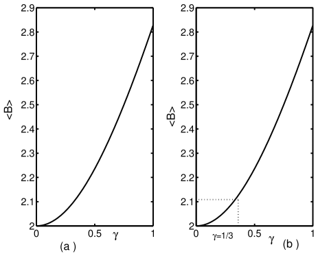
Figure 1: Plot of the maximum violation of our Bell inequality versus $\gamma$. (a) corresponds to the state $\varrho_{m}$ which shows the inequality can be violated for all $\gamma>0$; (b) corresponds to the Werner state, i.e. the state $\varrho_{w}(\gamma,\pi/4)$, which shows that our inequality can be violated for all $\gamma>1/3$. (b) also shows the inequality can be violated for $\gamma\leq 1/3$ due to the considered decomposition of $\varrho_{w}$

Another example is the variational Werner state introduced in Ref. [5] given by

$$\varrho_{w}(\gamma,\xi)=\frac{1-\gamma}{4}I_{2}\otimes I_{2}+\gamma\left|\Psi_{non}\right\rangle\left\langle\Psi_{non}\right|,$$ (12)

where $I_{2}\$is $(2\times 2)$-dimensional identity matrix and $\left|\Psi_{non}\right\rangle=\cos\xi\left|00\right\rangle+\sin\xi\left|11\right\rangle$. For $\xi=\frac{\pi}{4}$, eq. (12) is the usual Werner state which was the first state found to be entangled for $\gamma>\frac{1}{3}$[11,14] and not violate a Bell inequality for single states. The Werner state was shown to violate the Bell inequality in Ref. [11] only for its concurrence $C(\varrho_{w})>\sqrt{\frac{1}{3}}$. Consider a possible decomposition as

$$\varrho_{w}(\gamma,\pi/4) = \frac{1-\gamma}{4}\left(\left|\Phi^{+}\right\rangle\left\langle\Phi^{+}\right|+\left|\Psi^{+}\right\rangle\left\langle\Psi^{+}\right|\right.$$

$$\left.+\left|\Phi^{-}\right\rangle\left\langle\Phi^{-}\right|+\left|\Psi^{-}\right\rangle\left\langle\Psi^{-}\right|+\gamma\left|\Psi_{non}\right\rangle\left\langle\Psi_{non}\right|,\right)$$

and the analogous correlation function given by eq. (11), one can obtain the corresponding Bell inequality. By optimization to maximize the violation (see Fig. 2), one can find that the state $\varrho_{w}(\gamma)$ violates the Bell inequality for all $\gamma>\frac{1}{3}.$

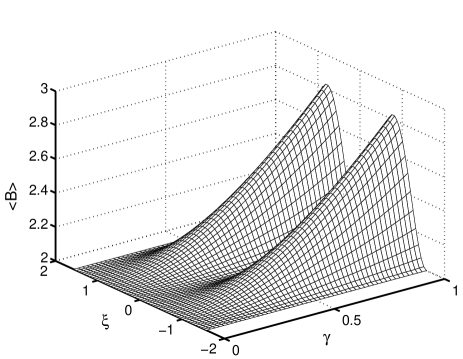
Figure 2: The maximum violation of our inequality for the variational Werner state $\varrho_{w}{(\gamma,\xi)}$ versus $\gamma$ and $\xi$. The figure shows the periodic violation of the state with $\xi$ and the violation with $\gamma$.

Above examples have shown that they violate our inequality by considering proper decompositions, although the original CHSH inequality is not violated. In our opinion, the key lies in the constraint on the Bell operator, $\left\langle ab\right\rangle-\left\langle ac\right\rangle$. I.e. the bound on the Bell operator in the original CHSH inequality is not tight enough for any entangled mixed state. Ours can be regarded as a correction of the bound. In this sense, we say our inequality is more refined.

What’s more, from Fig. 2 and Fig. 1 (b), it is so surprising that the inequality is violated not only for $\gamma>\frac{1}{3}$ but for all $\gamma>0$, which means a separable mixed state can also violate the inequality. It seems to be a paradox. In fact, it is not the case. The key lies in that our inequality depends on the decomposition of the density matrix. To better show the dependent relation, let us take a third density matrix as an example. Consider the bipartite density matrix given by

$$\varrho_{s}=\left(\begin{array}[]{cccc}\frac{1}{4}&0&0&x\\ 0&\frac{1}{4}&x&0\\ 0&x&\frac{1}{4}&0\\ x&0&0&\frac{1}{4}\end{array}\right),$$ (13)

with $\left|x\right|\leq\frac{1}{4}$, one can have $C(\varrho_{s})=0$ for all $\left|x\right|\leq\frac{1}{4}$. That is to say, $\varrho_{s}$ can expressed by the convex combination of product states, i.e.

$$\varrho_{1} = \varrho_{s}=\left(\frac{1}{4}+x\right)\left|\varphi\right\rangle\left\langle\varphi\right|\otimes\left|\varphi\right\rangle\left\langle\varphi\right|$$ (14)

$$+\left(\frac{1}{4}-x\right)\left|\varphi\right\rangle\left\langle\varphi\right|\otimes\left|\psi\right\rangle\left\langle\psi\right|$$

$$+\left(\frac{1}{4}-x\right)\left|\psi\right\rangle\left\langle\psi\right|\otimes\left|\varphi\right\rangle\left\langle\varphi\right|$$

$$+\left(\frac{1}{4}+x\right)\left|\psi\right\rangle\left\langle\psi\right|\otimes\left|\psi\right\rangle\left\langle\psi\right|,$$

where $\left|\varphi\right\rangle=\frac{1}{\sqrt{2}}\left(\left|0\right\rangle+\left|1\right\rangle\right)$ and $\left|\psi\right\rangle=\frac{1}{\sqrt{2}}\left(\left|0\right\rangle-\left|1\right\rangle\right)$. However, $\varrho$ can also obtained by the convex combination of maximally entangled states, i.e.

$$\varrho_{2} = \varrho_{s}=\left(\frac{1}{4}+x\right)\left(\left|\Phi^{+}\right\rangle\left\langle\Phi^{+}\right|+\left|\Psi^{+}\right\rangle\left\langle\Psi^{+}\right|\right)$$ (15)

$$+\left(\frac{1}{4}-x\right)\left(\left|\Phi^{-}\right\rangle\left\langle\Phi^{-}\right|+\left|\Psi^{-}\right\rangle\left\langle\Psi^{-}\right|\right).$$

Considering the same correlation functions and following the same procedure, based on the inequality (6), one can obtain the corresponding Bell inequality for eq. (14) and eq. (15), respectively. By our numerical optimization to maximize the violation of the inequalities for eq. (14) and eq. (15), respectively, given by Fig. 3, one can find that $\varrho_{2}$ always violate the inequality for $nozero$ $x$, while $\varrho_{1}$ is always constrained by the inequality for all $x$. This just shows the property that the current inequality depends on the decomposition of density matrix. In fact, if keeping it in mind that all pure states cannot violate the original CHSH inequality, one will easily find from the derivation of our inequality that a separable density matrix cannot violate our inequality if considering the product-state-decomposition.

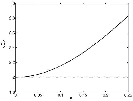
Figure 3: The maximum violation of our inequality for the separable state $\varrho_{s}$ versus $x$ in terms of two different decompositions. The figure shows that the inequality can be violated for the entangled-state decomposition (solid line) and can not be violated for the product-state decomposition (dotted line).

Since the violation of Bell inequality means there exists quantum correlation, our examples have shown that a separable mixed state may have quantum correlation which depends on the concrete realization of the state, even though the state has been defined as a separable one based on the usual entanglement measure such as concurrence and so on [17]. In fact, this is not strange. As mentioned in Ref. [5], the classical correlation does not mean the state has been prepared in the manner described, but only that its statistical properties can be reproduced by a classical mechanism. In other words, if considering the entanglement of pure states as a cost, the usual measurement of entanglement of formation for mixed states just gives the least cost to reproduce the mixed states. That is to say, the usual entanglement measure does not always extract quantum correlations that have been used to generate the given mixed state. I.e. The violation of our inequality means that quantum correlations are needed to produce the given mixed state by the considered concrete realization (decomposition). In this sense, we say that a separable mixed state may owe some quantum correlations. Therefore, in order to demonstrate whether a mixed state owe quantum correlations in terms of previous entanglement measures or whether our inequality is consistent with the usual entanglement measures, one has to test whether our inequality is violated in terms of the optimal decomposition in the sense of the given entanglement measure (for example, concurrence and so on).

In summary, we have presented a generalized Bell inequality. The inequality has been shown to be more refined than the previous ones. The most important property is that the inequality has a variable bound which depends on the decomposition of the state. As a result, a separable quantum mixed state may be shown to include quantum correlation, a potential understanding of which has been provided. Finally, we hope that the current result will further the understanding of quantum entanglement and quantum nonlocality.

Thank X. X. Yi, C. Li and Y. Q. Guo for their valuable discussions. This work was supported by the National Natural Science Foundation of China, under Grant Nos. 10575017 and 60472017.

References

(1) A. Einstein, B. Podolsky, and N. Rosen, Phys. Rev. 47, 777 (1935).
(2) S. L. Braunstein, A. Mann, and M. Revzen, Phys. Rev. Lett.
68, 3259 (1992).
(3) J. S. Bell, Physics (Long Island City, N.Y.) 1, 195
(1964).
(4) J. Clauser, M. Horne, A. Shimony, and R. Holt, Phys. Rev.
Lett. 23, 880 (1969).
(5) R. F. Werner, Phys. Rev. A 40, 4277 (1989).
(6) K. Banaszek and K. Wódkiewicz, Phys. Rev. A 58,
4345 (1998); Phys. Rev. Lett. 82, 2009 (1999); Acta Phys. Slovaca
49, 491 (1999).
(7) H. Jeong, J. Lee, and M. S. Kim, Phys. Rev. A 61,
052101 (2000).
(8) Zeng-Bing Chen, Jian-Wei Pan, Guang Hou and Yong-De Zhang,
Phys. Rev. Lett. 88, 040406 (2002).
(9) N. Gisin, Phys. Lett. A 145, 201 (1991).
(10) S. Popescu and D. Rohrlich, Phys. Lett. A 166, 293
(1992).
(11) N. Gisin and A. Peres, Phys. Lett. A 162, 15 (1992).
(12) S. L. Braunstein, A. Mann, and M. Revzen, J. Phys. A 25, L851 (1992).
(13) W. J. Munro, K. Nemoto and A. G. White, J. Mod. Opt. 48(7), 1239 (2001).
(14) A. G. White, D. V. F. James, W. J. Munro, and P. G. Kwiat,
(submitted to Nature).
(15) C. H. Bennett, G. Brassard, S. Popescu, B. Schumacher, and W.
K. Wootters, Phys. Rev. Lett. 76, 722 (1996).
(16) An alternate derivation can be obtained by considering the
convex combination of the CHSH inequalities which each pure state of the
density matrix satisfies and utilizing the absolute value inequality.
(17) W. K. Wootters, Phys. Rev. Lett. 80, 2245 (1998);
and the references therein.