Fault-tolerant quantum computation with high threshold in two dimensions

Abstract

We present a scheme of fault-tolerant quantum computation for a local architecture in two spatial dimensions. The error threshold is 0.75% for each source in an error model with preparation, gate, storage and measurement errors.

Quantum computation is fragile. Exotic quantum states are created in the process, exhibiting entanglement among large numbers of particles across macroscopic distances. In realistic physical systems, decoherence acts to transform these states into more classical ones, compromising their computational power. Fortunately, the effects of decoherence can be counteracted by quantum error correction ShorE . In fact, arbitrarily large quantum computations can be performed with arbitrary accuracy, provided the error level of the elementary components of the quantum computer is below a certain threshold. This is guaranteed by the threshold theorem for quantum computation TT1 ; TT2 ; TT3 ; TT4 .

Now that the threshold theorem has been established, it is important to devise methods for error correction which yield a high threshold, are robust against variations of the error model, and can be implemented with small operational overhead. An additional desideratum is a simple architecture for the quantum computer, requiring no long-range interaction, for example.

Recently, a threshold estimate of $3\times 10^{-2}$ per operation has been obtained for a method using post-selection Kn2 . An alternative scheme with high threshold combines topological quantum computation with state purification BT . (See also BMD .) In that approach, a subset of the universal gates are assumed to be error-free. Pure topological quantum computation ideally requires no error correction but often picks up a comparable poly-logarithmic overhead SKoh in the Solovay-Kitaev construction for approximating single- and two-qubit gates (c.f. Bon ). fault tolerance is more difficult to achieve in architectures where each qubit can only interact with other qubits in its immediate neighborhood. A fault tolerance threshold for a two-dimensional lattice of qubits with only local and nearest-neighbor gates is $1.9\times 10^{-5}$ Svo .

In this Letter, we present a scheme for fault-tolerant universal quantum computation on a two-dimensional lattice of qubits, requiring only a nearest-neighbor translation-invariant Ising interaction and single-qubit preparation and measurement. A fault tolerance threshold of $7.5\times 10^{-3}$ for each error source is presented, with moderate resource scaling. This scheme is best suited for implementation with massive qubits where geometric constraints naturally play a role, such as cold atoms in optical lattices Ola or two-dimensional ion traps Hen .

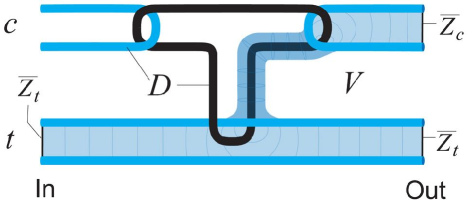
Figure 1: (Color online.) The CNOT gate $\Lambda(X)_{c,t}$ ($c$: control, $t$: target) formed by topologically entangled lattice defects. Each pair of defects carries an encoded qubit. Defects exist as primal (blue) and dual (black), and are created by local measurement. The primal correlation surface (light blue) shown here converts an incoming Pauli operator $Z_{t}$ into an outgoing $Z_{t}\otimes Z_{c}$, as required for a CNOT gate.

The presented scheme integrates methods of topological quantum computation, specifically the toric code Kit1 , and magic state distillation BK04 into the one-way quantum computer ($QC_{\cal{C}}$) RBB03 on cluster states. By employing magic state distillation we improve the error threshold significantly beyond RHG , with the threshold value and overhead scaling now set by the topological error correction. In this regard, we would like to emphasize that the three-dimensional cluster state is an intrinsically fault-tolerant substrate for quantum computation RHG . From the viewpoint of implementation it is desirable to reduce the spatial dimensionality of the scheme from three to two. To achieve this we turn the $QC_{\cal{C}}\;$into a sequential scheme in which the cluster state is created slice by slice.

This Letter is organized as follows. First, we construct fault-tolerant universal gates for the $QC_{\cal{C}}\;$in three spatial dimensions. (See Fig. 1 for a CNOT gate.) Next, we perform the mapping to two dimensions. Finally, we present our error model and work out its threshold value.

We consider a cluster state $|\phi\rangle_{\cal{L}}$ on a lattice ${\cal{L}}$ with elementary cell as displayed in Fig. 2a. Qubits are located at the center of faces and edges of ${\cal{L}}$. The lattice ${\cal{L}}$ is subdivided into three regions $V$, $D$ and $S$. Each region has its purpose, shape and specific measurement basis for its qubits. The qubits in $V$ are measured in the $X$-basis, the qubits in $D$ in the $Z$-basis, and the qubits in $S$ in either the $Y$-basis or the eigenbasis $(X+Y)/\sqrt{2}$. $V$ fills up most of the cluster. $D$ is composed of thick line-like structures, named defects. $S$ is composed of well-separated qubit locations interspersed among the defects. As described in greater detail below, the cluster region $V$ provides topological error correction, while regions $D$ and $S$ specify the Clifford and non-Clifford parts of a quantum algorithm, respectively.

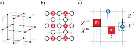
Figure 2: (Color online.) Lattice definitions. a) Elementary cell of the cluster lattice ${\cal{L}}$. 1-chains of ${\cal{L}}$ (dashed lines), and graph edges (solid lines). b) A surface code obtained from a 2D cluster state by local $X$-measurements. c) A pair of electric (“e”) or magnetic (“m”) holes in the code plane each support an encoded qubit. $\overline{Z}^{e/m}$ and $\overline{X}^{e/m}$ denote the encoded Pauli operators $Z$ and $X$, respectively.

We can break up this measurement pattern into gate simulations by establishing the following correspondence: $\mbox{\em{quantum gates}}\leftrightarrow\mbox{\em{quantum correlations}}\leftrightarrow\mbox{\em{surfaces}}$, as illustrated for the CNOT gate in Fig. 1. The first part of this correspondence has been established in RBB03 . For the second part homology comes into play. The correlations of $|\phi\rangle_{\cal{L}}$ (i.e., the stabilizers) can be identified with 2-chains (surfaces) in ${\cal{L}}$, while errors map to 1-chains (lines). Homological equivalence of the chains implies physical equivalence of the corresponding operators RHG . This correspondence is key to the presented scheme. Gates are specified by a set of surfaces with input and output boundaries, and syndrome measurements correspond to closed surfaces (having no boundary).

Formally, ${\cal{L}}$ is regarded as a chain complex, ${\cal{L}}=\{C_{3},C_{2},C_{1},C_{0}\}$. It has a dual ${\overline{\cal{L}}}=\{\overline{C}_{3},\overline{C}_{2},\overline{C}_{1},\overline{C}_{0}\}$ whose cubes $\overline{c}_{3}\in\overline{C}_{3}$ map to sites $c_{0}\in C_{0}$ of ${\cal{L}}$, whose faces $\overline{c}_{2}\in\overline{C}_{2}$ map to edges $c_{1}\in C_{1}$ of ${\cal{L}}$, etc. The chains have coefficients in $\mathbb{Z}_{2}$. One may switch back and forth between ${\cal{L}}$ and $\overline{\cal{L}}$ by a duality transformation $\mbox{}^{*}(\;)$. ${\cal{L}}$, $\overline{\cal{L}}$ are equipped with a boundary map $\partial$, where $\partial\circ\partial=0$.

Operators may be associated with chains as follows. Suppose that for each qubit location $a$ in a chain $c$, $a\in\{c\}$, there exists an operator $\Sigma_{a}$, with $[\Sigma_{a},\Sigma_{b}]=0$ for all $a,b\in\{c\}$. Then, we define $\Sigma(c):=\prod_{a\in\{c\}}\Sigma_{a}$. Cluster state correlations are associated with 2-chains. Specifically, all elements in the cluster state stabilizer take the form $K(c_{2})K(\overline{c}_{2})$ with $c_{2}\in C_{2}$, $\overline{c}_{2}\in\overline{C}_{2}$, and $K(c_{2})=X(c_{2})Z(\partial c_{2}),\;\;K(\overline{c}_{2})=X(\overline{c}_{2})Z(\partial\overline{c}_{2}).$ Only those stabilizer elements compatible with the local measurement scheme are useful for information processing. In particular, they need to commute with the measurements in $V$ and $D$,

$$\begin{array}[]{rclcr}{[K(c_{2})K(\overline{c}_{2}),X_{a}]}&=&0,&&a\in V,\\ {[K(c_{2})K(\overline{c}_{2}),Z_{b}]}&=&0,&&b\in D.\end{array}$$ (1)

This condition may again be expressed in terms of the chains $c_{2}$, $\overline{c}_{2}$ directly, which we will do below.

Topological error correction in $V$.

Inside $V$ the constraint (1) implies $\partial c_{2}=0$, $\partial\overline{c}_{2}=0$. In particular, these conditions are obeyed for $c_{2}=\partial c_{3}$, $\overline{c}_{2}=\partial\overline{c}_{3}$. For each elementary cube $q\in C_{3}$, $\overline{q}\in\overline{C}_{3}$ the cluster stabilizers $K(\partial q)$, $K(\partial\overline{q})$ can be measured by the local $X$-measurement and classical post-processing.

The optimal error correction procedure for $V$ can be mapped to a model from classical statistical mechanics, the random plaquette $\mathbb{Z}_{2}$-gauge model in three dimensions (3D-RPGM) DKLP , for which a fault tolerance threshold of $3.3\times 10^{-2}$ for local noise has been found in numerical simulations Ohno . (See also TSN .) Here we use the minimum weight chain matching algorithm AlgoEff for error correction. It yields a slightly smaller threshold of $2.9\times 10^{-2}$ Harri but is computationally efficient. Various error sources eat away at this 3% error budget.

Cluster states and surface codes.

The connection between a 2D cluster state and a surface code is illustrated in Fig. 2b. The extra spatial dimension in a 3D cluster state allows to evolve coded states in “simulated time”. The number of qubits which can be encoded in a surface code depends solely on the surface topology. Here we consider a plane with pairs of either electric or magnetic holes; see Fig. 2c. A magnetic hole is a plaquette $f$ where the associated stabilizer generator $S_{\Box}(f)=Z(\partial{f})$ is not enforced on the code space, and an electric hole is a site $s$ where the associated stabilizer $S_{+}(s)=X(\partial\mbox{ }^{\#}s)$ is not enforced on the code space, where “$\#$” denotes the duality transformation in 2D. Each hole is the intersection of a defect strand with a constant-time slice.

A pair of holes supports a qubit. For a pair of magnetic holes $f,f^{\prime}$, the encoded spin flip operator is $\overline{X}^{m}=X(\overline{c}_{1})$, with $\{\partial\overline{c}_{1}\}=\{\mbox{}^{\#}f,\mbox{}^{\#}f^{\prime}\}$, and the encoded phase flip operator is $\overline{Z}^{m}=Z(c_{1})$, with $c_{1}\cong\partial f$ or $c_{1}\cong\partial f^{\prime}$. The operator $Z(\partial f+\partial f^{\prime})$ is in the code stabilizer. For a pair of electric holes $s,s^{\prime}$ we have $\overline{X}^{e}=X(\overline{c}_{1}^{\prime})$, with $\overline{c}_{1}^{\prime}\cong\partial\mbox{}^{\#}s$, $\overline{Z}^{e}=Z(c_{1})$, with $\{\partial c_{1}\}=\{s,s^{\prime}\}$, and $X(\partial\mbox{}^{\#}s+\partial\mbox{}^{\#}s^{\prime})$ is in the code stabilizer.

Quantum logic.

The CNOT gate is realized by linking primal and dual defects as displayed in Fig. 1. To explain the functioning of the gate we refer to Theorem 1 of RBB03 . We consider a block shaped cluster ${\cal{C}}$ where the elementary cell of Fig. 2a is repeated an integer number of times along each direction. One of these directions is singled out as “simulated time”. The two perpendicular slices of the cluster at the earliest and latest times contain the supports $I$ and $O$ for the encoded input and output qubits, respectively, with $I,O\subset\{C_{1}\}$ encoded by the surface code of Fig. 2c.

The set $M$ on which the measurement pattern is defined (c.f. Thm 1 of RBB03 ) is composed of $V$ and $D$, $M=V\cup D$. Due to the presence of a primal lattice ${\cal{L}}$ and a dual lattice $\overline{\cal{L}}$, it is convenient to subdivide the sets $V$ and $D$ into primal and dual subsets. Specifically, $V=V_{p}\cup V_{d}$, with $V_{p}\subset\{C_{2}\}$, $V_{d}\subset\{\overline{C}_{2}\}$, and $D=D_{p}\cup D_{d}$, with $D_{p}\subset\{C_{1}\}$, $D_{d}\subset\{\overline{C}_{1}\}$.

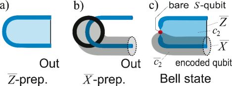
Figure 3: (Color online.) Remaining gates for universal fault-tolerant computation. The relevant correlation surfaces are shown in light blue and gray. Replace Out(put) by In(put) for a measurement. a) Preparation of a $\overline{Z}$-eigenstate for an electric qubit. b) Preparation of an $\overline{X}$-eigenstate for an electric qubit. c) Creation of a Bell pair among a bare $S$-qubit and an encoded qubit.

With these definitions, we can now prove the functioning of the CNOT gate in Fig. 1. The gate cluster ${\cal{C}}$ contains the regions $V_{p}$, $V_{d}$, $D_{p}$, $D_{d}$, $I$ and $O$. In this setting, condition (1) implies for the correlation surfaces:

$$\begin{array}[]{rclcrcl}\{c_{2}\}&\subset&V_{p},&&\{\partial c_{2}\}&\subset&D_{p}\cup I\cup O,\\ \{\overline{c}_{2}\}&\subset&V_{d}\cup I\cup O,&&\{\partial\overline{c}_{2}\}&\subset&D_{d}.\end{array}$$ (2)

One such (primal) correlation surface is depicted in Fig. 1. The corresponding stabilizer of $|\phi\rangle_{\cal{C}}$, after measurement of the qubits in $M=V\cup D$, implies a stabilizer $\pm\overline{Z}^{e}_{t,I}\overline{Z}^{e}_{c,O}\overline{Z}^{e}_{t,O}=\pm\overline{Z}^{e}_{t,I}\Lambda(X)_{c,t}\overline{Z}^{e}_{t,O}\Lambda(X)_{c,t}^{\dagger}$ for $|\Psi\rangle_{IO}$. Three similar surfaces imply the stabilizer elements $\pm\overline{X}^{e}_{t,I}\overline{X}^{e}_{t,O}$, $\pm\overline{Z}^{e}_{c,I}\overline{Z}^{e}_{c,O}$ and $\pm\overline{X}^{e}_{c,I}\overline{X}^{e}_{c,O}\overline{X}^{e}_{t,O}$ for $|\Psi\rangle_{IO}$. Theorem 1 of RBB03 is applied with $U=\Lambda(X)_{c,t}$. ∎

Further elements of a fault-tolerant $QC_{\cal{C}}$-computation are shown in Fig. 3. Fault-tolerant preparation of encoded $X$- and $Z$-eigenstates for the electric qubits are displayed in Figs. 3a and 3b, which can be reversed to denote measurements. These operations, together with the CNOT gate of Fig. 1, comprise the set of topologically protected gates. Fig. 3c shows the creation of a Bell pair between a bare $S$-qubit and a qubit encoded with a surface code (electric). The shown correlation surfaces $c_{2}$, $\overline{c}_{2}$ are such that $\{c_{2}\}\subset V_{p}$, $\{\partial c_{2}\}\subset D_{p}\cup S\cup O$, $\{\overline{c}_{2}\}\subset V_{d}\cup S\cup O$, $\{\partial\overline{c}_{2}\}=\emptyset$. The corresponding stabilizers $K(c_{2})$, $K(\overline{c}_{2})$ imply, after local measurement of the qubits in $V$ and $D$, the stabilizer generators $\pm Z_{S}\overline{Z}_{O}$, $\pm X_{S}\overline{X}_{O}$ for the state $|\Psi\rangle_{SO}$. Thus, $|\Psi\rangle_{SO}$ is a Bell state with the qubit located on $O$ being encoded. Measurement of the bare qubit on $S$ in the eigenbasis of $Y$ or $(X+Y)/\sqrt{2}$ yields on $O$ an encoded state $|\overline{Y}\rangle=|\overline{0}\rangle+i|\overline{1}\rangle$ or $|\overline{A}\rangle=|\overline{0}\rangle+e^{i\pi/4}|\overline{1}\rangle$, respectively. These states are noisy and therefore subsequently purified via magic state distillation BK04 . Finally, they are used in teleportation circuits (see Fig. 10.25 of NC00 ) to generate the fault-tolerant gates $\exp(i\pi/4\,\overline{X})$ and $\exp(i\pi/8\,\overline{Z})$. This completes the universal fault-tolerant gate set.

Mapping to the 2D lattice.

The dimensionality of the spatial layout can be reduced by one if the cluster is created slice by slice. That is, we convert the axis of “simulated time”—introduced as a means to explain the connection with surface codes—into real time.

Cluster qubits located on time-like edges of ${\cal{L}}$ or $\overline{\cal{L}}$ become syndrome qubits, which are periodically measured. Qubits on space-like edges become code qubits. Time-like oriented $\Lambda(Z)$ gates are mapped to Hadamard gates, while space-like oriented $\Lambda(Z)$ gates remain unchanged.

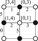
Figure 4: Elementary cell of the 2D lattice. Temporal order of operations in $V$: The labels on the edges denote the time steps at which the corresponding $\Lambda(Z)$ gate is performed. The labels at the syndrome vertices (“$\circ$”) denote measurement and (re-)preparation times $[t_{M},t_{P}]$, and the labels at the code vertices (“$\bullet$”) denote times for Hadamard gates $(t_{H},t_{H}^{\prime})$. The pattern is periodic in space, and in time with period six.

The temporal order of operations is displayed in Fig. 4. Note that every qubit is acted upon by an operation in every time step. The mapping to the two-dimensional structure has no impact on information processing. In particular, the error correction procedure is still the same as in fault-tolerant quantum memory with the toric code.

Error model and threshold.

There are two separate thresholds, one for the Clifford operations and one for the non-Clifford operations. The former threshold derives from topological error correction and the latter from magic state distillation. The overall threshold is set by the smaller of the two.

Mapping to a single-layer 2D structure slightly modifies the effective error model on the lattices ${\cal{L}}$ and $\overline{\cal{L}}$, as compared to RHG . Specifically, we assume the following: 1) Erroneous operations are modeled by perfect operations preceded or followed by a partially depolarizing single- or two-qubit error channel $T_{1}=(1-p_{1})[I]+p_{1}/3\,([X]+[Y]+[Z])$, $T_{2}=(1-p_{2})[I]+p_{2}/15\,([X_{a}X_{b}]+..+[Z_{a}Z_{b}])$. The error sources are a) the preparation of the individual qubit states $|+\rangle$ (error probability $p_{P}$), b) the Hadamard gates (error probability $p_{1}$), c) the $\Lambda(Z)$ gates (error probability $p_{2}$), d) measurement (error probability $p_{M}$). 2) Classical syndrome processing is instantaneous.

When calculating a threshold, we assume that all error sources are equally strong, $p_{1}=p_{2}=p_{M}=p_{P}:=p$. Storage errors need not be considered because no qubit is ever idle between preparation and measurement. This model encompasses realistic error sources such as local inhomogeneity of electric and magnetic fields, fluctuations in laser intensity, and imperfect photodetectors.

The topological threshold for each physical source is estimated by numerical simulations to be

$$p_{c}=7.5\times 10^{-3}.$$ (3)

A similar threshold persists under modifications of the error model such as higher weight errors RHG .

Regarding the distillation threshold, the residual error $\epsilon_{l}$ at level $l$ undergoes the recursion $\epsilon_{l}\rightarrow\epsilon_{l+1}=35{\epsilon_{l}}^{3}$ (to leading order) BK04 . The initial distillation error $\epsilon_{0}$ arises through the effective error on an $S$-qubit, with $\epsilon_{0}=6p$. The distillation threshold $p_{c}$ for each physical error source is then $p_{c}=1/6\sqrt{35}\approx 2.8\times 10^{-2}$. The purification threshold is much larger than the topological threshold, and therefore the overall threshold for fault-tolerant $QC_{\cal{C}}$-computation is given by Eq. (3).

Overhead.

fault tolerance leads to a poly-logarithmic increase of operational resources. Both the overheads in topological error correction and in magic state distillation are described by a characteristic exponent: $\gamma_{top}=3$ and $\gamma_{ms}=\log_{3}15$. The larger one dominates the resource scaling. Given bare circuit size $S$, the encoded circuit size $S^{\prime}$ scales as $S^{\prime}\sim S\log^{3}S$.

Conclusion.

We have presented a scheme of fault-tolerant quantum computation in a two-dimensional local architecture with high error threshold and moderate overhead in resource scaling. The threshold of $7.5\times 10^{-3}$ is the highest known for a local architecture. Our scheme only requires local and translation-invariant nearest-neighbor interaction in a single-layer two-dimensional lattice. Small-scale experimental devices may be realized in optical lattices, segmented ion traps, or arrays of quantum dots or superconducting qubits where short-range interaction is preferred.

- (1) P. W. Shor, Proc. 37th Annual Symp. on the Foundations of Computer Science, 56 (IEEE, Los Alamitos, 1996).
- (2) E. Knill, R. Laflamme, and W. H. Zurek, Proc. Roy. Soc. London A 454, 365 (1998).
- (3) D. Aharonov and M. Ben-Or, Proc. 29th Annual Symp. on Theory of Computing, 176 (ACM, New York, 1997); D. Aharonov and M. Ben-Or, quant-ph/9906129.
- (4) D. Gottesman, Ph.D. thesis, Caltech (1997), quant-ph/9705052.
- (5) P. Aliferis, D. Gottesman, and J. Preskill, Quant. Inf. Comp. 6, 97 (2006).
- (6) E. Knill, Nature 434, 39 (2005).
- (7) S. Bravyi, Phys. Rev. A 73, 042313 (2006).
- (8) H. Bombin and M. A. Delgado, Phys. Rev. Lett. 97, 180501 (2006); H. Bombin and M.A. Delgado, quant-ph/0610024.
- (9) C. M. Dawson and M. A. Nielsen, Quant. Inf. Comp. 6, 81 (2006).
- (10) D. Stepanenko and N. E. Bonesteel, Phys. Rev. Lett. 95, 140503 (2005).
- (11) K. M. Svore, D. P. DiVincenzo, and B. M. Terhal, quant-ph/0604090.
- (12) D. Jaksch et al., Phys. Rev. Lett. 82, 1975 (1999).
- (13) W. K. Hensinger et al., Appl. Phys. Lett. 88, 034101 (2006).
- (14) A. Kitaev, Ann. Phys. 303, 2 (2003).
- (15) S. Bravyi and A. Kitaev, Phys. Rev. A 71, 022316 (2005).
- (16) R. Raussendorf, D. E. Browne, and H. J. Briegel, Phys. Rev. A 68 (2003).
- (17) R. Raussendorf, J. Harrington, and K. Goyal, Ann. Phys. 321, 2242 (2006).
- (18) E. Dennis et al., J. Math. Phys. 43, 4452 (2002).
- (19) T. Ohno et al., Nucl. Phys. B 697, 462 (2004).
- (20) K. Takeda, T. Sasamoto and H. Nishimori, J. Phys. A 38, 3751 (2005).
- (21) J. Edmonds, Can. J. Math 17, 449 (1965).
- (22) C. Wang, J. Harrington, and J. Preskill, Ann. Phys. 303, 31 (2003).
- (23) S. Bravyi and A. Kitaev, quant-ph/9811052.
- (24) M. A. Nielsen and I. L. Chuang, Quantum Computation and Quantum Information (Cambridge University Press, Cambridge, UK, 2000).