A Model for an Irreversible Bias Current in the Superconducting Qubit Measurement Process.

Abstract

The superconducting charge-phase ‘Quantronium’ qubit is considered in order to develop a model for the measurement process used in the experiment of Vion et. al. [Science 296 886 (2002)]. For this model we propose a method for including the bias current in the read-out process in a fundamentally irreversible way, which to first order, is approximated by the Josephson junction tilted-washboard potential phenomenology. The decohering bias current is introduced in the form of a Lindblad operator and the Wigner function for the current biased read-out Josephson junction is derived and analyzed. During the read-out current pulse used in the Quantronium experiment we find that the coherence of the qubit initially prepared in a symmetric superposition state is lost at a time of 0.2 nanoseconds after the bias current pulse has been applied. A timescale which is much shorter than the experimental readout time. Additionally we look at the effect of Johnson-Nyquist noise with zero mean from the current source during the qubit manipulation and show that the decoherence due to the irreversible bias current description is an order of magnitude smaller than that found through adding noise to the reversible tilted washboard potential model. Our irreversible bias current model is also applicable to the persistent current based qubits where the state is measured according to its flux via a small inductance direct current superconducting quantum interference device (DC-SQUID).

I Introduction

Quantum computers and the quantum algorithms that run on them have been proposed as a technology to perform computational tasks not tractable with classical computer circuitsneilsen . Recent experiments have provided significant advances towards developing the fundamental element of this technology, the quantum bit or qubit. So far, qubit systems based on nuclear magnetic resonanceNMR1 ; NMR2 and ion trapsionTraps ; ionTraps2 have been used to show multiple qubit operation, whilst efficient linear optic quantum computingKLM has been demonstrated with the successful operation of the two qubit controlled-not gateUQCNOT . Experimental advances have also been made in solid state systems which utilise a wide variety of quantum effects in many different materials. The main attraction of solid state systems is the possibility to scale such technology using modern-day device fabrication techniques once the implementation of component gates has been demonstrated. Promising solid state systems include the use of phosphor dopants in siliconkane , charge based quantum dotsblick ; Fujisawa ; Kouwenhouven , optically controlled exciton systemsXLiScience301-809 as well as a variety of systems based on the coherent electron state in superconducting materialsreview .

In these superconducting systems the implementation of single qubit operationnakamura ; Martinis ; Yu ; delft ; Vion , some with single shot readout, has been demonstrated. Also devices with a non-switchable inter-qubit interaction between two qubits have been shownpaskin ; Maryland , providing the initial evidence for a two-qubit entangled state in these structures. To ensure scalability to more complex configurations into the future there is a need to identify ways to develop more accurate gates, provide higher fidelity readout and ensure longer coherence times in the devices being developed. For instance the ‘Quantronium’ charge-phase qubit developed by Vion et al.Vion was designed to be insensitive to first order fluctuations in the external control parameters of the system provided that the control parameters for the device, in this case the voltage and applied flux, were used about an ‘optimal point’ of the system with this property. In this experiment the quality factor of quantum coherence Q for the device, defined as the number of elementary gate operations that could be performed before the device state decoheres, was found to be of the order $10^{4}$.

In this paper we examine the readout process in the experiment of Vion et. al. through the Lindblad operator formalismlimblad and we introduce the bias current into the model in a fundamentally irreversible way that acts to decohere the state of the qubit. Using this method we implement a heuristic model for the measurement process that is induced by the application of the bias current to the quantronium circuit. This model allows for the bias current to ‘count’ the number of electrons that pass through the system during the measurement process and in doing so destroys the coherence between the different states of the system. Therefore to examine this model we are ignoring the typical terms which appear in the system master equation that describe the widely known forms of decoherence for the qubit through its coupling to the environment, such as the ohmic dissipation of the leadsleggett . Our aim is to gain further insight into the role of the irreversible readout process and the decohering process associated with its operation.

The irreversible dynamics arising from the current bias provides a decoherence mechanism that collapses the quantum superposition to a probabilistic mixture on a time scale shorter than the time for the state to tunnel out of the metastable qubit states into unbound states of the washboard potential and create a voltage on the read-out voltmeter. This means that the measurement of the system is performed during the application of the bias current before any classical information about the qubit state is returned to the experimentalist. Such ‘measurement induced decoherence’ is analogous to that discussed in semiconducting systemsstace:136802 . In addition to this we also analyse the implications this irreversible current source has for the effect of Johnson-Nyquist noise from the current source during the qubit manipulation when the bias current has a zero mean and intended to be decoupled form the device.

II The Current Biased Josephson Junction

The measurement process in superconducting qubit structures such as the Quantronium and the direct current superconducting quantum interference device (DC-SQUID) (which is used to measure the persistent current qubitsdelft and proposed to measure magnetic nanoparticlesspiller2 ) rely upon the transition of a Josephson junction based system from the superconducting state into the voltage state, where the information associated with the effective critical current of the device provides the quantum state measurement. The semi-classical model for a single Josephson junction is the one-dimensional analogy to a particle of mass $(\hbar/2e)^{2}C$ moving along the $\gamma$ axis in the potentialtinkham

$$U(\gamma)=E_{J}(1-\cos\gamma)-E_{b}\gamma,$$ (1)

where $E_{b}=I_{bias}\Phi_{0}/2\pi$. The $E_{b}\gamma$ term describes the slope of the washboard potential, which has been used widely in the quantum regimeleggett . For instance, it has been used to describe the escape rates of macroscopic tunnelling events in current biased Josephson junctionsMartinis2 ; Martinis3 . The inclusion of the linear potential in Eq. (1) to create the tilted washboard potential does not contribute any dephasing term to the dynamics and implies that the measurement process is intrinsically reversible. That is, by turning the current source on and then off again, the qubit is back in its initial state (provided a macroscopic quantum tunnelling event has not occurred).

In this paper we propose an alternate description of the current bias in the Quantronium and other current biased systems such as the DC-SQUID, one which gives rise to the washboard potential $E_{b}\gamma$ term as well as intrinsically irreversible dynamics. This irreversiblity arises as a direct consequence of the measurement process, and the starting point for our model is the master equation

$$\overset{.}{\rho}=-\frac{i}{\hbar}[H,\rho]+L\rho L^{\dagger}-\frac{L^{\dagger}L\rho}{2}-\frac{\rho L^{\dagger}L}{2},$$ (2)

where for $I_{bias}>0$ we have defined $L=\sqrt{|E_{b}|/\hbar}\eta^{\dagger}$ (see referencespiller ) and the charge-tunnelling non-unitary operator on the large Josephson junction is $\eta^{\dagger}\left|n\right\rangle=\left|n+1\right\rangle$ and $\eta\left|n\right\rangle=\left|n-1\right\rangle$. The state $|n\rangle$ represents the number of Cooper pairs that have tunnelled through the large Josephson junction (i.e an eigenstate of the Cooper pair number operator $N$) and the cooper pair tunnelling operator $\eta$ satisfies $\left[N,\eta^{\dagger}\right]=\eta^{\dagger}$ and $\left[N,\eta\right]=-\eta$. For $I_{bias}<0$ we have defined $L=\sqrt{|E_{b}|/\hbar}\eta$. These Lindblad operators account for the movement of Cooper pairs across the Josephson junction at an average rate given by the current $I_{bias}/2e$. That is, the operators $\eta^{\dagger}$ and $\eta$ count the number of electrons added by the external bias current to the large Josephson junction at an average rate $|E_{b}|/\hbar$.

By introducing the Lindblad equation, given by Eq. (2), we are proposing a heuristic method to model the bias current which attempts to capture the notion that the current source counts the number of electrons tunnelling through the Josephson junction. In the remainder of this section we reconcile such a model by showing that it is in fact in agreement with a classical current biased Josephson junction and that the Lindblad terms contained in Eq. (2) tend to destroy superpositions of different phase states.

Using Eq. (2), the master equation therefore reads

$$\overset{.}{\rho}=\left\{\begin{array}[]{rl}-\frac{i}{\hbar}[H,\rho]+\frac{|E_{b}|}{\hbar}\left(\eta^{\dagger}\rho\eta-\rho\right)&\text{ if }I_{bias}\geq 0\\ -\frac{i}{\hbar}[H,\rho]+\frac{|E_{b}|}{\hbar}\left(\eta\rho\eta^{\dagger}-\rho\right)&\text{ if }I_{bias}<0.\end{array}\right.$$ (3)

In this equation the Hamiltonian $H$ describes the Josephson junction or qubit dynamics but does not include the bias current washboard potential terms. Describing the current bias in superconducting circuits through this Lindblad superoperator is compatible with the phenomenology of the current biased Josephson junction in the classical limit $(C\rightarrow\infty)$ where the phase across the Josephson junction is fixed by the applied current. For instance, we can consider a single Josephson junction which is current biased ($I_{bias}\geq 0$) and described by Eq. (3) where the Hamiltonian is given by

$$H=\frac{2e^{2}}{C}N^{2}+\frac{\Phi_{0}I_{C}}{2\pi}\left(1-\cos{\gamma}\right)$$

and $N$ is the Cooper pair number operator on the Josephson junction. In the steady state of this equation for the single Josephson junction, $\overset{.}{\rho}=0$, we can compute the quantity

$$\frac{d\left\langle N\right\rangle}{dt}=\operatorname{Tr}(\overset{.}{\rho}N)=0,$$

to look at the role of the bias current in our model. Using the cyclic property of the trace we find that

$$-i\operatorname{Tr}(\rho\left[N,H\right])+|E_{b}|\operatorname{Tr}(\eta^{\dagger}\rho\left(N+1\right)\eta-\rho N)=0$$

and from the commutation relations for $\eta$ and $N$, together with the definition of the current operator

$$I =\frac{2\pi}{\Phi_{0}}\frac{\partial H}{\partial\gamma}=I_{C}\sin\gamma$$

$$=I_{C}\left(\frac{\eta^{\dagger}-\eta}{2i}\right)=\frac{2i\pi}{\Phi_{0}}\left[N,H\right],$$ (4)

we therefore show for $I_{bias}\geq 0$ that we have the expected result in the classical limit $(C\rightarrow\infty)$; that is

$$\left\langle I\right\rangle=\operatorname{Tr}(\rho I)=I_{bias}.$$

Also by considering an oppositely biased current ($I_{bias}<0$) we find that by the inclusion of the Lindblad terms for the bias current in the master equation (Eq. (3)) we have $\left\langle I\right\rangle=I_{bias}$ and therefore retained the expected behaviour of the the bias current in the single Josephson junction system. That is, the current through the Josephson junction in our model is that applied by the current source.

Additionally, in our model, the linear washboard term $E_{b}\gamma$ arises naturally from the Lindblad superoperator description of the bias current. By expanding the Lindblad superoperators in terms of its phase representation, then to first order, we can obtain the reversible dynamics of the washboard potential through the $E_{b}\gamma$ term. The higher-order terms from this expansion provide us with the intrinsic irreversible terms of the current source in our model. Hence having introduced the current source as an irreversible one, the system can be approximated by the washboard potential model of a current biased Josephson junction with an added irreversibility. For instance, by making an approximation to the full master equation (Eq. (3)) for the Quantronium circuit we can write the operators $\eta^{\dagger}$ and $\eta$ in their phase representation and approximate them to second order. That is we can write

$$\eta^{\dagger}=e^{+i\gamma}\approx 1+i\gamma-\frac{\gamma^{2}}{2}$$ (5)

and

$$\eta=e^{-i\gamma}\approx 1-i\gamma-\frac{\gamma^{2}}{2}.$$ (6)

Under this approximation, and considering the cases for $I_{bias}$ being positive and negative, the master equation of the system is

$$\overset{.}{\rho}=-\frac{i}{\hbar}[H-E_{b}\gamma,\rho]+\frac{|E_{b}|}{\hbar}\left(\gamma\rho\gamma-\frac{\gamma^{2}\rho}{2}-\frac{\rho\gamma^{2}}{2}\right).$$ (7)

Here we emphasise that the first order approximation to the operator $L$ is the $E_{b}\gamma$ term which appears in the tilted washboard potential model. The additional three terms appearing at the end of the master equation are the irreversible decohering terms of this model under our second order approximation.

By making the second order approximations (Eq. (5) and Eq. (6)) for the operators $\eta^{\dagger}$ and $\eta$, we have expanded them in terms of the operator $\gamma$ about the point $\langle\gamma\rangle=0$; in this expansion we have used the small parameter $\Delta$ which is the variance of a sharply peaked Gaussian state in the phase representation. For instance if we consider only the decoherence term in the $I_{bias}>0$ master equation (Eq. (3)) we have

$$\overset{.}{\rho}=\frac{|E_{b}|}{\hbar}\left(e^{+i\gamma}\rho e^{-i\gamma}-\rho\right)=\frac{|E_{b}|}{\hbar}{\mathcal{D}}[\gamma]\rho.$$ (8)

The steady state of this master equation can be written as $\rho_{0}=|\psi_{0}\rangle\langle\psi_{0}|$ where $|\psi_{0}\rangle$ is the sharply peaked Gaussian steady state wavefunction. This wavefunction results from the small charging energy relative to the Josephson energy of the junction. Note that this wavefunction, tightly peaked around a given value of $\gamma$, is consistent with the Josephson relation for a classical current passing through a Josephson junction. Therefore we write the steady state wave function as

$$\left|\psi_{0}\right\rangle=\frac{1}{\sqrt[4]{2\pi\Delta}}\int e^{-\gamma^{2}/4\Delta}\left|\gamma\right\rangle d\gamma,$$

where the variance $\Delta$ is small so that the wavefunction is sharply peaked in phase. Using this wavefunction to construct the steady state density matrix $\rho_{0}$ we can approximate the term ${\mathcal{D}}[\gamma]\rho_{0}$ in the master equation (Eq. (8)) as follows:

$${\mathcal{D}}[\gamma]\rho_{0}= \frac{1}{\sqrt{2\pi\Delta}}\int e^{i(\gamma-\gamma^{\prime})-\frac{\gamma^{2}+\gamma^{\prime 2}}{4\Delta}}\left|\gamma\right\rangle\left\langle\gamma^{\prime}\right|d\gamma^{\prime}d\gamma-\left|\psi_{0}\right\rangle\left\langle\psi_{0}|\right.$$

$$= -i\sqrt{\Delta}\left[-\overset{\_}{\gamma},\rho_{0}\right]-\Delta\left[\overset{\_}{\gamma},\left[\overset{\_}{\gamma},\rho\right]\right]+O\left[\Delta^{3/2}\right],$$

where we have used the scaled phase operator $\gamma=\sqrt{\Delta}\overset{\_}{\gamma}$, and we have approximated the exponential by its Taylor series expanded in terms of the small parameter $\sqrt{\Delta}$. After also considering the case $I_{bias}<0$, we approximate the Lindblad derived decoherence term in the master equation as

$$\overset{.}{\rho}=-i\sqrt{\Delta}\frac{E_{b}}{\hbar}\left[-\overset{\_}{\gamma},\rho\right]-\Delta\frac{|E_{b}|}{\hbar}\left[\overset{\_}{\gamma},\left[\overset{\_}{\gamma},\rho\right]\right]+O\left[\Delta^{3/2}\right]$$

so that in the limit that $E_{b}\rightarrow\infty$ and $\sqrt{\Delta}\rightarrow 0$ then $\sqrt{\Delta}E_{b}/\hbar$ is a constant $\widetilde{E}_{b}/\hbar$. In this limit the master equation is

$$\overset{.}{\rho}=-\frac{i}{\hbar}[-\widetilde{E_{b}}\overset{\_}{\gamma},\rho],$$

which is the washboard potential arising from the bias-current. Thus the tilted washboard term arises naturally from our master equation, accompanied by an intrinsically irreversible part.

III The Quantronium Measurement Model

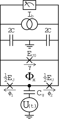
Figure 1: Circuit diagram of the Quantronium qubit.

In order to apply our irreversible current source approach to recent experiments we consider the Quantronium qubit system depicted in Fig. 1. The design of this charge-phase qubit is similar to that of the Cooper pair box transistorJoyezPRL72-2458 . The device consists of two identical low capacitance Josephson junctions with a coupling energy $E_{J}/2$ and capacitance $C_{J}/2$. These junctions are on either side of the isolated superconducting charge ‘island’ which is in a state of paired electron charge $2eN$, where $N$ is the number of Cooper pairs on the island. This island is incorporated into a superconducting loop with a larger Josephson junction, which by design, has a coupling energy of $E_{J0}\sim 20E_{J}$ and a large shunt capacitance $C$; which was used in the experiment to reduce phase fluctuations. The design of this device requires that the characteristic energies $E_{J}$ and the charging energy $E_{C}=2e^{2}/(C_{J}+C_{g}^{\prime})$, where $1/C_{g}^{\prime}=1/C_{g}+1/4C$, are comparable so that neither charge or quantised flux states in the loop are good quantum numbers. The discrete energy states of the device are quantum superpositions of several charge statescottet ; cottetThesis . Control of the qubit is made via the pulsed microwave voltage source $U(t)$ which is capacitively coupled to the Cooper pair box by the capacitor $C_{g}$, and the applied flux $\Phi_{x}$ through the three junction superconducting loop. These provide the elementary single qubit manipulations.

For this device the relation $\delta=\gamma+2e\Phi_{x}/\hbar$ between the combined phase $\delta=\phi_{1}-\phi_{2}$ across the Josephson junctions of the Cooper pair box, and the phase $\gamma$ across the larger Josephson junction provides the readout process of the Quantronium quantum state. From this relation the two lowest energy states of the Quantronium have different persistent currents in the three junction loop. This difference is used for state readout, a current pulse $I_{bias}(t)$ from the ‘ideal’ current source is applied where the height of the pulse is chosen so that the transition to a voltage state is made for only one of the Quantronium energy eigenstates; when the addition of the loop persistent current state and the current pulse exceeds the critical current of the large junction. This process discriminates between the two qubit states associated with the two lowest levels of the Quantronium.

The Hamiltonian for the Quantronium, which we consider in terms of the master equation Eq. (3) and its approximation Eq. (7), that is without the energy term corresponding to the readout current source $I_{bias}$ is

$$H= \phantom{+}E_{C}(N-N_{g})^{2}+E_{J}\left(1-\cos\left(\frac{\phi+\gamma}{2}\right)\cos{\varphi}\right)$$

$$+\frac{Q^{2}}{2C}+E_{J0}\left(1-\cos\gamma\right).$$

Here we have used the terms: the phase operator $\varphi=(\phi_{1}+\phi_{2})/2$ which is conjugate to the Cooper pair number operator $N$, the dimensionless gate charge $N_{g}=C_{g}U/2e$, the phase bias $\phi=2\pi\Phi_{x}/\Phi_{0}$ where $\Phi_{0}=h/2e$ is the flux quantum, and the charge $Q$ on the large Josephson junction with shunt capacitance $C$. In this Hamiltonian we have neglected the energy term corresponding to the loop inductance of the device based on the size of the device.

To analyse the measurement induced decoherence in our model we simplify the Hamiltonian $H$ by considering the dynamics of the lowest two qubit eigenstates where we use $|0\rangle$ and $|1\rangle$ to denote the lowest and first excited state of the Quantronium system respectively. Here we work at the point where the applied flux $\Phi_{x}$ is set to 0 and the dimensionless gate charge $N_{g}$ is set to $1/2$. In this configuration the qubit energy levels are separated by the Josephson Junction coupling energy so we write our Hamiltonian as

$$H^{\prime}= \phantom{+}E_{J}\left(1-\cos\left(\frac{\gamma}{2}\right)\right)\sigma_{z}+E_{C0}N^{2}$$

$$+E_{J0}\left(1-\cos\gamma\right),$$ (9)

where $E_{C0}=2e^{2}/C$ and $N$ is the charge operator for the large Josephson junction which is conjugate to the phase operator $\gamma$. This Hamiltonian describes a two level system separated by an energy $E_{J}(1-\cos(\gamma/2))$ where the phase $\gamma$ provides the coupling between the qubit and the readout junction. If we now assume that the large junction is in a localised semi-classical state near $\langle\gamma\rangle=0$, then by expanding $\cos\gamma$ in Eq. (9) to second order in $\gamma$, we obtain the Hamiltonian

$$H_{R}=E_{C0}N^{2}+\frac{E_{J0}\gamma^{2}}{2}+\frac{E_{J}\gamma^{2}\sigma_{z}}{8},$$ (10)

which has a form of a displaced simple harmonic oscillator.

IV The DC-SQUID Measurement Model

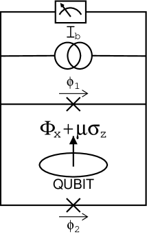
Figure 2: Circuit diagram of a DC-SQUID used for qubit state detection via a measurement of the qubit’s magnetic flux.

In addition to the Quantronium experiments our approach is applicable to the systems where a two level quantum device has been measured by a small inductance DC-SQUID such as the persistent current qubitdelft . In these experiments the coherent oscillations in a low inductance three Josephson junction qubit structure have been observed. Similarly, the use of low inductance microSQUIDMicroSQUID structures have been proposed to readout the quantum state of nanometre scale magnetic particles of large spin and high anisotropy molecular clustersspiller2 . Here the measurement of a magnetic flux quantum state inductively coupled to a DC-SQUID with a low inductance relies on the induced change of the effective critical current of the the DC-SQUID, for this type of measurement a current ramp scheme is used which is similar to that used in the Quantronium readout process.

In Fig. 2 we consider two Josephson junctions with a coupling strength $E_{J0}/2$, capacitance $C_{J0}/2$ and phases (as shown) of $\phi_{1}$ and $\phi_{2}$ in a superconducting loop. For this device we define the total phase $\gamma=(\phi_{1}+\phi_{2})/2$ across the device and the applied flux

$$2\pi\left(\frac{\Phi_{x}-\mu\,\sigma_{z}}{\Phi_{0}}\right)=\phi_{1}-\phi_{2}$$

where $\mu\sigma_{z}$ is the magnetic flux of the qubit state. When the loop inductance is small then the flux through the loop $\Phi\approx\Phi_{x}-\mu\,\sigma_{z}$, also when the charging energy of the Josephson junctions is small so that the quantum state of the DC-SQUID detector is well defined in phase and the energy of the first excited state of the detector is larger than the other energies of the system so that it exhibits ground state behaviour, then we can write the Hamiltonian of the system for the master equation Eq. (3) and its approximation Eq. (7) as

$$H=H_{Q}+H_{S},$$

here the DC-SQUID Hamiltonian is

$$H_{S}=\frac{\left(e\,N\right)^{2}}{2C_{J0}}+E_{J0}\,(1-\cos\gamma\,\cos(\varphi_{x}-\delta\varphi\,\sigma_{z}))$$

where $\varphi_{x}-\delta\varphi\,\sigma_{z}=\pi(\Phi_{x}-\mu\,\sigma_{z})/\Phi_{0}$ and the qubit Hamiltonian is $H_{Q}=(\epsilon_{0}\,\sigma_{z}+t_{0}\,\sigma_{x})/2.$ For small $\delta\varphi$, eliminating the constant terms and assuming that the tunnelling between the flux states of the qubit has been turned off, $t_{0}=0$, we simplify this Hamiltonian $H$ to

$$H^{\prime}= \phantom{-}\frac{\epsilon_{0}}{2}\,\sigma_{z}+E_{C0}\,N^{2}-E_{J0}\,\cos\varphi_{x}\,\cos{\gamma}$$

$$-E_{J0}\,\delta\varphi\,\sigma_{z}\,\sin\varphi_{x}\,\cos{\gamma}.$$

This Hamiltonian is similar to Eq. (9), and since we assume that the DC-SQUID is localised near $\langle\gamma\rangle=0$ we again make a second order approximation to the $\gamma$ terms to arrive at the reduced Hamiltonian

$$H_{\mathrm{R}}=E_{C0}\,N^{2}+\frac{E_{J0}\,\cos\varphi_{x}\,\gamma^{2}}{2}+\frac{E_{J0}\,\delta\varphi\,\sin\varphi_{x}\,\gamma^{2}\,\sigma_{z}}{2},$$

when the qubit energy level separation satisfies $\epsilon_{0}/2=E_{J0}\,\delta\varphi\,\sin\varphi_{x}$. Since the form of this Hamiltonian is identical to Eq. (10) then the model presented for the Quantronium can be directly applied to the measurement of the magnetic flux of a qubit with a low inductance DC-SQUID.

V The Reversible Current Source

V.1 The Reversible Current Source Wigner Function

To investigate the Hamiltonian dynamics of the Quantronium measurement model (and by analogy the DC-SQUID measurement model) we consider the simplified Quantronium Hamiltonian derived in the previous section:

$$H_{R}=E_{C0}\,N^{2}+\frac{E_{J0}\,\gamma^{2}}{2}+\frac{E_{J}\,\gamma^{2}\,\sigma_{z}}{8}.$$ (11)

We use this Hamiltonian to analyse the measurement induced decoherence relative to the washboard potential phenomenology, which does not include the effects of decoherence. In this section we derive the decoherence-free dynamics of the system using the standard tilted-washboard model by including the term $E_{b}\gamma$ in the Hamiltonian Eq. (11). In this model, the density matrix for the qubit and the readout device evolves according to

$$\overset{.}{\rho}=-\frac{i}{\hbar}[H_{R}-E_{b}\gamma,\rho].$$ (12)

We decompose $\rho$ as

$$\rho= \phantom{+}\rho_{+}(t)\otimes\left|0\right\rangle\left\langle 0\right|+\rho_{\times}(t)\otimes\left|0\right\rangle\left\langle 1\right|$$

$$+{\rho_{\times}}^{\dagger}(t)\otimes\left|1\right\rangle\left\langle 0\right|+\rho_{-}(t)\otimes\left|1\right\rangle\left\langle 1\right|,$$ (13)

where $\rho_{+}$ and $\rho_{-}$ describe the evolution of the Josephson junction when the qubit is in the states $|0\rangle$ and $|1\rangle$ whilst $\rho_{\times}$ describes the coherence between them. We assume the initial state of the system $\rho(0)$ is a product state of the readout Josephson junction density matrix $w$ and the qubit in the symmetric state $(|0\rangle+|1\rangle)/\sqrt{2}$, so

$$\rho(0)=\frac{w(0)}{2}\otimes\left(|0\right\rangle\left\langle 0|+|0\right\rangle\left\langle 1|+|1\right\rangle\left\langle 0|+|1\right\rangle\left\langle 1|\right).$$

The dynamics of $\rho_{+}$ and $\rho_{-}$ do not depend on $\rho_{\times}$, so their dynamics are described by the qubit-state dependent Hamiltonian

$$H_{R\pm}=E_{C0}N^{2}+\frac{E_{J0}\gamma^{2}}{2}\pm\frac{E_{J}\gamma^{2}}{8}.$$

We define the two sets of raising and lowering operators $a_{\pm}^{\dagger}$ and $a_{\pm}$ by

$$\gamma=\Gamma_{\pm}(a_{\pm}^{\dagger}+a_{\pm})=\sqrt{\frac{\lambda_{\pm}}{2}}\left(a_{\pm}^{\dagger}+a_{\pm}\right)$$ (14)

and

$$N=-\frac{i}{\sqrt{2\lambda_{\pm}}}\left(a_{\pm}-a_{\pm}^{\dagger}\right),$$ (15)

where $\lambda_{\pm}=\sqrt{2\nu/{(1\pm\mu/4)}}$, $\nu=E_{C0}/E_{J0}$, $\mu=E_{J}/E_{J0}$, and $H_{R\pm}=\hbar\omega_{\pm}a_{\pm}^{\dagger}a_{\pm}$ where

$$\hbar\omega_{\pm}=\sqrt{2E_{C0}E_{J0}\left(1\pm\frac{E_{J}}{4E_{J0}}\right)}.$$

Using these scalings we can define the two independent equations for $\rho_{+}$ and $\rho_{-}$

$$\overset{.}{\rho}_{+} =-i\left[\omega_{+}a_{+}^{\dagger}a_{+}-\frac{E_{b}\Gamma_{+}}{\hbar}\left(a_{+}^{\dagger}+a_{+}\right),\rho_{+}\right]$$ (16)

$$\overset{.}{\rho}_{-} =-i\left[\omega_{-}a_{-}^{\dagger}a_{-}-\frac{E_{b}\Gamma_{-}}{\hbar}\left(a_{-}^{\dagger}+a_{-}\right),\rho_{-}\right].$$ (17)

By the anti-commutation relation, $\{A,B\}=AB+BA$, we define the equation for the off-diagonal element $\rho_{\times}$ as

$$\overset{.}{\rho}_{\times}= -i\left[\omega_{\times}a_{\times}^{\dagger}a_{\times}-\frac{E_{b}\Gamma_{\times}}{\hbar}\left(a_{\times}^{\dagger}+a_{\times}\right),\rho_{\times}\right]$$

$$-i\frac{E_{J}{\Gamma_{\times}}^{2}}{8\hbar}\left\{\left(a_{\times}^{\dagger}+a_{\times}\right)^{2},\rho_{\times}\right\}.$$ (18)

For the off-diagonal component $\rho_{\times}$ we have defined the raising and lowering operators $a_{\times}^{\dagger}$ and $a_{\times}$ where

$$\gamma=\Gamma_{\times}(a_{\times}^{\dagger}+a_{\times})=\sqrt{\frac{\lambda_{\times}}{2}}\left(a_{\times}^{\dagger}+a_{\times}\right),$$ (19)

$$N=-\frac{i}{\sqrt{2\lambda_{\times}}}\left(a_{\times}-a_{\times}^{\dagger}\right),$$ (20)

$\lambda_{\times}=\sqrt{2\nu}$, and $\hbar\omega_{\times}=\sqrt{2E_{C0}E_{J0}}.$ The master equation for $\rho_{\times}$ defines the dynamics of both the off-diagonal elements of the density matrix, where the equation for ${\rho_{\times}}^{*}$ is the Hermitian conjugate of Eq. (18).

To solve the dynamics of the system, we transform to a Wigner representation of the statewigner ; milburn . To obtain the equation of motion for the Wigner function we first derive the characteristic function equation of motion $\partial\Upsilon(\beta)/\partial t=\operatorname{Tr}(D\overset{.}{\rho})$, where the characteristic function is defined as $\Upsilon(\beta)=\operatorname{Tr}(\operatorname{D\rho})$ and $D$ is the displacement operator defined by $D=\exp(\beta a^{\dagger}-\beta^{*}a)$. Writing $D$ in normal and anti-normal order then we can find the relevant operator rules for converting to the characteristic function equations. The Wigner function equation of motion is found by taking the Fourier transform of the characteristic function equation of motion $\overset{.}{\Upsilon}(\beta)$. Thus

$$\overset{.}{W}(\alpha)=\int_{-\infty}^{+\infty}e^{\beta^{*}\alpha-\beta\alpha^{*}}\overset{.}{\Upsilon}(\beta)d^{2}\beta.$$ (21)

After performing this procedure we use a compact notation to write down the Wigner function equations from the three master equations Eq. (16) - Eq. (18); for the operators $a_{+}$, $a_{-}$ and $a_{\times}$ defined in the three master equations we correspondingly have the complex parameters $\alpha_{+}$, $\alpha_{-}$ and $\alpha_{\times}$ but we drop the subscripts since they appear separately in the three characteristic function equations. This procedure provides us with three uncoupled equations

$$\overset{.}{W}_{+}(\alpha)= -i\omega_{+}(\partial_{\alpha^{*}}\alpha^{*}-\partial_{\alpha}\alpha)W_{+}(\alpha)$$

$$-\frac{iE_{b}\Gamma_{+}}{\hbar}\left(\partial_{\alpha}-\partial_{\alpha^{*}}\right)W_{+}(\alpha),$$ (22)

$$\overset{.}{W}_{-}(\alpha)= -i\omega_{-}(\partial_{\alpha^{*}}\alpha^{*}-\partial_{\alpha}\alpha)W_{-}(\alpha)$$

$$-\frac{iE_{b}\Gamma_{-}}{\hbar}\left(\partial_{\alpha}-\partial_{\alpha^{*}}\right)W_{-}(\alpha),$$ (23)

$$\overset{.}{W}_{\times}(\alpha)= -i\omega_{\times}(\partial_{\alpha^{*}}\alpha^{*}-\partial_{\alpha}\alpha)W_{\times}(\alpha)$$

$$-\frac{iE_{b}\Gamma_{\times}}{\hbar}\left(\partial_{\alpha}-\partial_{\alpha^{*}}\right)W_{\times}(\alpha)$$

$$-\frac{iE_{J}{\Gamma_{\times}}^{2}}{8\hbar}\left(2\left(\alpha^{*}\right)^{2}+2\alpha^{2}+4|\alpha|^{2}\right)W_{\times}(\alpha)$$

$$-\frac{iE_{J}{\Gamma_{\times}}^{2}}{16\hbar}\left(\partial_{\alpha^{*}}^{2}+\partial_{\alpha}^{2}-2\partial_{\alpha}\partial_{\alpha^{*}}\right)W_{\times}(\alpha).$$ (24)

We note that each of these three equations are described in three separate co-ordinate spaces related to each other by a small scaling factor. This same procedure will be used in the description of the irreversible current source described in the following section. Eq. (24) can be expressed in terms of the phase $\gamma$ and charge $N$ variables using the definitions Eq. (14) and Eq. (15), doing so we find

$$\overset{.}{W}_{\times}(\gamma,N)= -\omega_{\times}\left(\lambda_{\times}\partial_{\gamma}N-\frac{1}{\lambda_{\times}}\partial_{N}\gamma\right)W_{\times}(\gamma,N)$$

$$-\frac{E_{b}}{\hbar}\partial_{N}W_{\times}(\gamma,N)$$

$$-\frac{iE_{J}}{16\hbar}\left(4\gamma^{2}-\partial_{N}^{2}\right)W_{\times}(\gamma,N).$$ (25)

V.2 The Reversible Current Source Wigner Function Solution

The first two Wigner function equations (Eq. (22) and Eq. (23)) for the readout Josephson junction density matrix component elements $\rho_{+}$ and $\rho_{-}$ can be solved analytically using the Wang and Uhlenbeck solution for a linear Fokker-Plank equationWangMilburn since the equations are of the form

$$\overset{.}{W}_{\pm}(\alpha_{\pm},t)=\left(-\nabla_{z}^{T}.M_{\pm}.z+\nabla_{z}^{T}.N_{\pm}.\nabla_{z}/2\right)W_{\pm}(\alpha_{\pm},t).$$ (26)

where

$$M_{\pm}=\left(\begin{array}[]{cc}-i\omega_{\pm}&0\\ 0&i\omega_{\pm}\end{array}\right),N_{\pm}=0,$$ (29)

$$\nabla_{z}=\binom{\partial_{\widetilde{\alpha}}}{\partial_{\widetilde{\alpha}^{*}}},z=\binom{\widetilde{\alpha}}{\widetilde{\alpha}^{*}},$$

and $\widetilde{\alpha}=\alpha-E_{b}\Gamma_{\pm}/(\hbar\omega_{\pm})$. From these two solutions $W_{+}$ and $W_{-}$ we can specify the Wigner function for the reduced state of the readout junction, since from the definition of the Wigner function we have

$$W(\gamma,N,t)= \int_{-\infty}^{+\infty}e^{\beta^{*}\alpha-\beta\alpha^{*}}\operatorname{Tr}(D\rho)d^{2}\beta$$

$$= \frac{1}{2}\left(W_{+}+W_{-}\right),$$ (30)

where the trace is performed over the Josephson junction and qubit states. From the Wigner function we can obtain a probability distribution for the state of the system in the state variables $\gamma$ or $N$ by integrating over the state variable for the state variable $N$ or $\gamma$ respectively.

This Wigner function for the combined system does not show the coherence that exists between the states of the qubit, that is it cannot be used to distinguish between a pure and a mixed state. We therefore construct a function from the three equations for the Wigner function terms $W_{+}\text{}$, $W_{-}$ and $W_{\times}$ that we derived from the readout Josephson junction density matrix component elements $\rho_{+}$, $\rho_{-}$, and $\rho_{\times}$; this function is found by directly Wigner transforming both sides of Eq. (13) over the Josephson junction degrees of freedom which defines the operator

$$\hat{W}_{s}(\gamma,N,t)= \phantom{+}W_{+}|0\left\rangle\right\langle 0|+W_{-}|1\left\rangle\right\langle 1|$$

$$+{W_{\times}}^{*}|1\left\rangle\right\langle 0|+W_{\times}|0\left\rangle\right\langle 1|.$$

From this we can calculate the projection onto the initial state $W_{s}(\gamma,N,t)=\left\langle+\right|\hat{W}_{s}(\gamma,N,t)\left|+\right\rangle$ where $\left|+\right\rangle=\left(\left|1\right\rangle+\left|0\right\rangle\right)/\sqrt{2}$ so that

$$W_{s}(\gamma,N,t)=\frac{1}{2}\left(W_{+}+W_{-}\right)+\operatorname{Re}(W_{\times}).$$

Integrating this function over the canonical coordinates gives the probability to find the system in the initial state at time $t$.

The solutions for the diagonal Wigner function terms $W_{+}$ and $W_{-}$ obtained from the Eq. (22) and Eq. (23) are the Gaussians

$$W_{\pm}(\alpha_{\pm},t)=\frac{1}{2\pi|C_{\pm}|}\exp\left(-\frac{1}{2}{u_{\pm}}^{T}.C_{\pm}^{-1}.u_{\pm}\right),$$ (31)

where

$$u_{\pm}(\alpha_{\pm},t)=\left(\begin{array}[]{c}\alpha_{\pm}-\frac{E_{b}\Gamma_{\pm}}{\hbar\omega_{\pm}}-e^{-i\omega_{\pm}t}\left(\alpha_{0}-\frac{E_{b}\Gamma_{\pm}}{\hbar\omega_{\pm}}\right)\\ \alpha_{\pm}^{*}-\frac{E_{b}\Gamma_{\pm}}{\hbar\omega_{\pm}}-e^{+i\omega_{\pm}t}\left(\alpha_{0}^{*}-\frac{E_{b}\Gamma_{\pm}}{\hbar\omega_{\pm}}\right)\\ \end{array}\right)$$

and the covariance matrix

$$C_{\pm}=\left(\begin{array}[]{cc}e^{-i\omega_{\pm}t}&0\\ 0&e^{i\omega_{\pm}t}\end{array}\right).C_{0}.\left(\begin{array}[]{cc}e^{-i\omega_{\pm}t}&0\\ 0&e^{i\omega_{\pm}t}\end{array}\right)$$

which decays from the initial covariance matrix:

$$C_{0}=\left(\begin{array}[]{cc}\left\langle\alpha^{2}\rangle_{0}\right.-\left\langle\alpha\rangle_{0}\right.^{2}&\left\langle|\alpha|^{2}\rangle_{0}\right.-|\left\langle\alpha\rangle_{0}\right.|^{2}\\ \left\langle|\alpha|^{2}\rangle_{0}\right.-|\left\langle\alpha\rangle_{0}\right.|^{2}&\left\langle\left(\alpha^{*}\right)^{2}\right\rangle_{0}-\left\langle\alpha^{*}\rangle_{0}\right.^{2}\end{array}\right)$$

The solution (Eq. (31)) for the terms $W_{+}$ and $W_{-}$ correspond to Gaussian functions in the $(\alpha_{\pm},\alpha_{\pm}^{*})$ co-ordinate space. The initial state of the Josephson junction at $t=0$ is a Gaussian centred about zero, so that at the instant the bias current $I_{bias}$ is applied

$$W_{s}(\alpha_{\times},0)= \frac{2}{\pi}\exp\left(-2\alpha_{\times}\alpha_{\times}^{*}\right)$$

$$= \frac{2}{\pi}\exp\left(-\frac{\gamma^{2}}{\lambda_{\times}}-\lambda_{\times}N^{2}\right),$$ (32)

this initial condition implies $\alpha_{0}=0$, and the covariance matrix

$$C_{\pm}=C_{0} =\frac{1}{4\lambda_{\pm}\lambda_{\times}}\left(\begin{array}[]{cc}{\lambda_{\times}}^{2}-{\lambda_{\pm}}^{2}&{\lambda_{\pm}}^{2}+{\lambda_{\times}}^{2}\\ {\lambda_{\pm}}^{2}+{\lambda_{\times}}^{2}&{\lambda_{\times}}^{2}-{\lambda_{\pm}}^{2}\end{array}\right)$$ (35)

$$\overset{\operatorname*{\textup{Lim}}\limits_{E_{\textup{J0}}\gg E_{J}}}{\longrightarrow}\left(\begin{array}[]{cc}0&1/2\\ 1/2&0\end{array}\right).$$ (38)

From the analytic solutions for the diagonal Wigner function terms $W_{+}$ and $W_{-}$ we see that they correspond to fixed width Gaussian curves that rotate on elliptical orbits through the $(\gamma,N)$ co-ordinate space at different frequencies $\omega_{+}$ and $\omega_{-}$ and the centre of the orbits are located at $E_{b}\Gamma_{+}/(\hbar\omega_{+})$ and $E_{b}\Gamma_{-}/(\hbar\omega_{-})$ along the phase axis respectively. These diagonal Wigner function terms in the absence of decoherence maintain their width and hence their noise characteristics during their evolution. Hence the Wigner function follows a complicated periodic motion. For instance, after a certain number of oscillations at time $2T_{0}=2\pi/(\omega_{+}-\omega_{-})$ the Wigner function term $W_{+}$ with the larger frequency $\omega_{+}$ has completed an extra oscillation about its elliptical orbit compared to the Wigner function term $W_{-}$.

For the off-diagonal Wigner function term $W_{\times}(\gamma,N,t)$ we assume a solution of the form

$$W_{\times}(\gamma,N,t)=\exp( a(t)\gamma+b(t)N+c(t)\gamma^{2}$$

$$+d(t)\gamma N+e(t)N^{2}+f(t)).$$ (39)

From Eq. (25), the coefficients in the exponent evolve according to

$$\overset{.}{a}(t) =\frac{\omega}{\lambda_{\times}}b(t)+Gd(t)+\frac{\left(-I+iE\right)}{2}b(t)d(t),$$ (40)

$$\overset{.}{b}(t) =-\lambda_{\times}\omega a(t)+2Ge(t)+\left(-I+iE\right)e(t)b(t),$$ (41)

$$\overset{.}{c}(t) =\frac{\omega}{\lambda_{\times}}d(t)-iE+\frac{\left(-I+iE\right)}{4}d(t)^{2},$$ (42)

$$\overset{.}{d}(t) =-2\lambda_{\times}\omega c(t)+\frac{2\omega}{\lambda_{\times}}e(t)+\left(-I+iE\right)e(t)d(t),$$ (43)

$$\overset{.}{e}(t) =-\lambda_{\times}\omega d(t)+\left(-I+iE\right)e(t)^{2},$$ (44)

$$\overset{.}{f}(t) =Gb(t)+\frac{\left(-I+iE\right)}{4}\left(2e(t)+b(t)^{2}\right),$$ (45)

where $G=-E_{b}/\hbar$, $E=E_{J}/4\hbar$ and $I=0$. Using the initial conditions $a(0)=0$, $b(0)=0$, $c(0)=-1/\lambda_{\times}$, $d(0)=0$, $e(0)=-\lambda_{\times}$, $f(0)=\ln(1/\pi)$ we can solve for $W_{\times}(\gamma,N,t)$ numerically.

The plot of the full Wigner function $W_{s}(\gamma,N,t)$ for the readout Josephson junction is plotted using the experimental parameters of the Quantronium experimentcottetThesis in Fig. 3. The interference fringes, centrally located between the two Gaussians $W_{+}$ and $W_{-}$, is due to the coherence between the qubit states, arising from $W_{\times}$. The number of interference fringes present at a particular time $t$ is related to the separation of the two Gaussians in the $(\gamma,N)$ co-ordinate space, which increases the further the terms $W_{+}$ and $W_{-}$ are apart. As the Gaussians separate the centre of the off-diagonal Wigner term $W_{\times}$ follows the trajectory shown in Fig. 5. In these figures we see that the main feature of these plots is that the noise properties and the interference fringes are conserved over time. In the absence of decoherence they continuously evolve with a complicated periodic motion. This will be contrasted against the evolution of the state in the presence of the irreversible bias current decoherence in the next section.

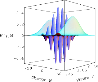
Figure 3: Plot of the full Wigner Function $W_{s}(\gamma,N,t)$ for the readout Josephson junction. The parameters used in this plot are taken from the Quantronium experimentVion ; cottetThesis and they are: $E_{J}=0.86k_{b}K$, $E_{C}=0.68k_{b}K$, $\text{}E_{\textup{C0}}=0.0037k_{b}K$, $E_{\textup{J0}}=18.4k_{b}K$ and $E_{b}=0.97E_{\textup{J0}}$ The time after which the bias current of $0.77\mu A$ is applied for this plot is $t=16.932\operatorname{ns}$. The plot demonstrates the different terms that appear in the decoherence free Wigner function for the readout Josephson junction. In the plot we can see that at this particular time the two Gaussian curves corresponding to the diagonal Wigner function terms $W_{+}$ and $W_{-}$ are separated and the interference fringes that correspond to the off-diagonal coherence term $\operatorname{Re}(W_{\times})$ appears between them.

(a)

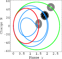
(b)

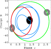
Figure 4: Contour plots of the decoherence free Wigner function $W_{s}(\gamma,N,t)$ with the trajectories of the centre of the three Wigner function components $W_{+}(\gamma,N,t)$, $W_{-}(\gamma,N,t)$ and $\operatorname{Re}(W_{\times}(\gamma,N,t))$ superimposed in red, green and blue respectively. (a) The contour plot of the three Wigner function terms is for time $t=T_{0}/4$. (b) The contour plot is for time $t=T_{0}$. Where the time $T_{0}$ is defined as the time when the diagonal terms $W_{+}(\gamma,N,t)$ and $W_{-}(\gamma,N,t)$ are the most separated and sit on opposite sides of their respective trajectory ellipse, $T_{0}=\pi/(\omega_{+}-\omega_{-})$. The parameters used in this plot are based on those from the Quantronium experiment and they are: $E_{J}=25\times 0.86k_{b}K$, $E_{C}=0.68k_{b}K$, $\text{}E_{\textup{C0}}=0.0037k_{b}K$, $E_{\textup{J0}}=18.4k_{b}K$ and $E_{b}=0.97E_{\textup{J0}}$; here the qubit energy $E_{J}$ has been increased by a factor of 25 in order to exaggerate the difference between the trajectories of the $W_{+}(\gamma,N,t)$ and $W_{-}(\gamma,N,t)$ terms. In these plots with the absence of decoherence the Wigner functions continuously evolve, moving about their respective trajectories maintaining their height and shape and hence conserving the equal probabilities of finding the system in either of the two qubit states which is consistent with the qubit symmetric superposition state $(|0\rangle+|1\rangle)/\sqrt{2}$. The superimposed trajectories are shown from time $t=0$ until $t=2T_{0}$

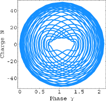
Figure 5: Parametric plot of the trajectory of the centre of the off-diagonal Wigner function term $W_{\times}(\gamma,N,t)$ for the parameters used in Fig. 4. Here the trajectory is shown from $t=0$ to $t=20\times T_{0}$ where $T_{0}=\pi/(\omega_{+}-\omega_{-})$. From this plot we see the continual coherence of the Wigner function under the absence of decoherence, since the off-diagonal $W_{\times}(\gamma,N,t)$ term continuously evolves in the co-ordinate space without decay.

VI The Irreversible Current Source - Measurement Induced Decoherence

VI.1 The Irreversible Current Source Wigner Function Equation

In the previous section the behaviour of the Quantronium system under the application of a bias current, introduced as a Hamiltonian term, was examined. Now we investigate the effect of an irreversible bias current model by adding the Lindblad derived terms that appear in Eq. (7) to show the relative decoherence in the system’s evolution. In this case we have the system density matrix $\rho$ defined by the master equation

$$\overset{.}{\rho}=-\frac{i}{\hbar}[H_{R}-E_{b}\gamma,\rho]-\frac{|E_{b}|}{2\hbar}[\gamma,\left[\gamma,\rho\right]].$$

Using the scaling factors Eq. (14) and Eq. (19) we can write the following three master equations to describe the elements of the density matrix $\rho$ as

$$\overset{.}{\rho}_{+}= -i\left[\omega_{+}a_{+}^{\dagger}a_{+}-\frac{E_{b}\Gamma_{+}}{\hbar}\left(a_{+}^{\dagger}+a_{+}\right),\rho_{+}\right]$$

$$-\frac{|E_{b}|{\Gamma_{+}}^{2}}{2\hbar}\left[a_{+}^{\dagger}+a_{+},\left[a_{+}^{\dagger}+a_{+},\rho_{+}\right]\right],$$

$$\overset{.}{\rho}_{-}= -i\left[\omega_{-}a_{-}^{\dagger}a_{-}-\frac{E_{b}\Gamma_{-}}{\hbar}\left(a_{-}^{\dagger}+a_{-}\right),\rho_{-}\right]$$

$$-\frac{|E_{b}|{\Gamma_{-}}^{2}}{2\hbar}\left[a_{-}^{\dagger}+a_{-},\left[a_{-}^{\dagger}+a_{-},\rho_{-}\right]\right],$$

$$\overset{.}{\rho}_{\times}= -i\left[\omega_{\times}a_{\times}^{\dagger}a_{\times}-\frac{E_{b}\Gamma_{\times}}{\hbar}\left(a_{\times}^{\dagger}+a_{\times}\right),\rho_{\times}\right]$$

$$-\frac{|E_{b}|{\Gamma_{\times}}^{2}}{2\hbar}\left[a_{\times}^{\dagger}+a_{\times},\left[a_{\times}^{\dagger}+a_{\times},\rho_{\times}\right]\right]$$

$$-\frac{iE_{J}{\Gamma_{\times}}^{2}}{8\hbar}\left\{\left(a_{\times}^{\dagger}+a_{\times}\right)^{2},\rho_{\times}\right\}.$$

Following the same procedure used in Section V we obtain the three component Wigner function equations. The three uncoupled Wigner function term equations are

$$\overset{.}{W}_{+}(\alpha)= -i\omega_{+}(\partial_{\alpha^{*}}\alpha^{*}-\partial_{\alpha}\alpha)W_{+}(\alpha)$$

$$-\frac{|E_{b}|{\Gamma_{+}}^{2}}{2\hbar}\left(\partial_{\alpha^{*}}^{2}+\partial_{\alpha}^{2}-2\partial_{\alpha}\partial_{\alpha^{*}}\right)W_{+}(\alpha)$$

$$-\frac{iE_{b}\Gamma_{+}}{\hbar}\left(\partial_{\alpha}-\partial_{\alpha^{*}}\right)W_{+}(\alpha),$$ (46)

$$\overset{.}{W}_{-}(\alpha)= -i\omega_{-}(\partial_{\alpha^{*}}\alpha^{*}-\partial_{\alpha}\alpha)W_{-}(\alpha)$$

$$-\frac{|E_{b}|{\Gamma_{-}}^{2}}{2\hbar}\left(\partial_{\alpha^{*}}^{2}+\partial_{\alpha}^{2}-2\partial_{\alpha}\partial_{\alpha^{*}}\right)W_{-}(\alpha)$$

$$-\frac{iE_{b}\Gamma_{-}}{\hbar}\left(\partial_{\alpha}-\partial_{\alpha^{*}}\right)W_{-}(\alpha),$$ (47)

$$\overset{.}{W}_{\times}(\gamma,N)= -\omega_{\times}\left(\lambda_{\times}\partial_{\gamma}N-\frac{1}{\lambda_{\times}}\partial_{N}\gamma\right)W_{\times}(\gamma,N)$$

$$-\frac{E_{b}}{\hbar}\partial_{N}W_{\times}(\gamma,N)+\frac{|E_{b}|}{2\hbar}\partial_{N}^{2}W_{\times}(\gamma,N)$$

$$-\frac{iE_{J}}{16\hbar}\left(4\gamma^{2}-\partial_{N}^{2}\right)W_{\times}(\gamma,N),$$ (48)

where the simplified $\alpha$ notation convention from the previous section has again been used. By solving these three equations we can investigate the evolution of the Quantronium device in the presence of the irreversible bias current and in particular the decay of the off-diagonal term $W_{\times}$, that projects the qubit into one of its eigenstates with probabilities related to the initial state of the qubit.

VI.2 The Irreversible Current Source Wigner Function Solution

As was the case for the Hamiltonian evolution of the Quantronium system with the reversible bias current term, which we described in the previous section, the first two Wigner function equations (Eq. (46) and Eq. (47)) can be solved using the Wang and Uhlenbeck solution for a linear Fokker-Plank equation since the equations are in the form of Eq. (26) where

$$M_{\pm}=\left(\begin{array}[]{cc}i\left(\omega_{\pm}\pm\frac{E_{J}{\Gamma_{\pm}}^{2}}{4\hbar}\right)&i\frac{E_{J}{\Gamma_{\pm}}^{2}}{4\hbar}\\ i\frac{E_{J}{\Gamma_{\pm}}^{2}}{4\hbar}&i\left(\omega_{\pm}\pm\frac{E_{J}{\Gamma_{\pm}}^{2}}{4\hbar}\right)\end{array}\right),$$ (51)

$$N_{\pm}=\frac{1}{\hbar}\left(\begin{array}[]{cc}-|E_{b}|{\Gamma_{\pm}}^{2}&+|E_{b}|{\Gamma_{\pm}}^{2}\\ +|E_{b}|{\Gamma_{\pm}}^{2}&-|E_{b}|{\Gamma_{\pm}}^{2}\end{array}\right),$$ (54)

$$\nabla_{z}=\binom{\partial_{\widetilde{\alpha}}}{\partial_{\widetilde{\alpha}^{*}}},z=\binom{\widetilde{\alpha}}{\widetilde{\alpha}^{*}},$$

and $\widetilde{\alpha}=\alpha-E_{b}\Gamma_{\pm}/(\hbar\omega_{\pm})$. The solution for the diagonal Wigner function terms $W_{+}$ and $W_{-}$ is the again the Gaussian

$$W_{\pm}(\alpha_{\pm},t)=\frac{1}{2\pi|C_{\pm}|}\exp\left(-\frac{1}{2}{u_{\pm}}^{T}.C_{\pm}^{-1}.u_{\pm}\right),$$ (55)

where

$$u_{\pm}(\alpha_{\pm},t)=\left(\begin{array}[]{c}\alpha_{\pm}-\frac{E_{b}\Gamma_{\pm}}{\hbar\omega_{\pm}}-e^{-i\omega_{\pm}t}\left(\alpha_{0}-\frac{E_{b}\Gamma_{\pm}}{\hbar\omega_{\pm}}\right)\\ \alpha_{\pm}^{*}-\frac{E_{b}\Gamma_{\pm}}{\hbar\omega_{\pm}}-e^{+i\omega_{\pm}t}\left(\alpha_{0}^{*}-\frac{E_{b}\Gamma_{\pm}}{\hbar\omega_{\pm}}\right)\\ \end{array}\right)$$

and from the initial condition Eq. (32) we have $\alpha_{0}=0$ and the covariance matrix

$$C_{\pm}=\left(\begin{array}[]{cc}\frac{i|E_{b}|{\Gamma_{\pm}}^{2}}{4\hbar\omega_{\pm}}\left(1-e^{-2i\omega_{\pm}t}\right)&\frac{|E_{b}|{\Gamma_{\pm}}^{2}t}{2\hbar}\\ \frac{|E_{b}|{\Gamma_{\pm}}^{2}t}{2\hbar}&\frac{i|E_{b}|{\Gamma_{\pm}}^{2}}{4\hbar\omega_{\pm}}\left(e^{2i\omega_{\pm}t}-1\right)\end{array}\right)$$ (58)

$$+\left(\begin{array}[]{cc}e^{-i\omega_{\pm}t}&0\\ 0&e^{+i\omega_{\pm}t}\end{array}\right).C_{0}.\left(\begin{array}[]{cc}e^{-i\omega_{\pm}t}&0\\ 0&e^{+i\omega_{\pm}t}\end{array}\right)$$ (63)

which decays from the initial covariance matrix $C_{0}$ given by Eq. (38). The solutions $W_{+}$ and $W_{-}$ (and $W_{\times}$) are shown in Fig.  6, the parameters used in this figure are the same as those used in Fig. 4 and Fig. 5, where the parameters of the Quantronium experiment have been used to demonstrate the evolution of the Wigner function with the exception that the qubit energy $E_{J}$ has been increased by a factor of 25 to exaggerate the separation of the states in the presence of the increasing noise characteristics of the irreversible bias current.

In Fig. 6 we see that the trajectories of the diagonal Wigner terms $W_{+}$ and $W_{-}$ through the $(\gamma,N)$ co-ordinate space are identical to those found using the reversible bias current approach of the previous section. With the application of the bias current $I_{bias}$ the two Gaussians start from the initial condition where they superimposed on each other at the origin and then $W_{+}$ and $W_{-}$ separate as they begin to rotate about the points $E_{b}\Gamma_{+}/\hbar\omega_{+}$ and $E_{b}\Gamma_{-}/\hbar\omega_{-}$ on the phase axis with a frequency $\omega_{+}$ and $\omega_{-}$ respectively. However, the shape and hence the noise characteristics of the $W_{+}$ and $W_{-}$ terms have changed. The off-diagonal elements $|E_{b}|{\Gamma_{\pm}}^{2}t/2\hbar$ in the covariance matrix Eq. (63) mean that during the evolution of the states, energy from the system is ‘leaking’ and causing the Gaussians to become broader as they separate. For long time this means that the states become virtually indistinguishable in the $(\gamma,N)$ co-ordinate space.

For the off-diagonal term $W_{\times}(\gamma,N)$ we solve Eq. (48) with a solution in the non-positive definite form Eq. (39). Using this form of solution we can derive the set of six coupled differential equations Eq. (40) - Eq. (45) where $G=-E_{b}/\hbar$, $I=-2|E_{b}|/\hbar$ and $E=E_{J}/4\hbar$. We can solve this set of equations numerically using the same initial conditions used in the previous section, i.e. Eq. (32). In Fig. 6 we see that $W_{\times}$ decays as the system evolves, so that by the time the diagonal terms $W_{+}$ and $W_{-}$ are the most separated at time $T_{0}$ it has virtually decayed to zero relative to the diffusing and larger diagonal Wigner terms. From this numerical solution of the off-diagonal Wigner function term $W_{\times}$ we are now in a position where we can examine the time it takes for the coherence of the initial qubit symmetric superposition state to be lost. Also the effect that this description of the bias current as a Poisson distributed kick process has on the qubit when white noise in current source is considered.

(a)

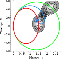
(b)

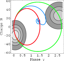
Figure 6: Contour plots of the Wigner function $W_{s}(\gamma,N,t)$ in the presence of the decoherence from the irreversible bias current. (a) Contour plot at time $t=T_{0}/4$. (b) Contour plot at time $t=T_{0}$ where $T_{0}=\pi/(\omega_{+}-\omega_{-})$. The superimposed trajectories show the time evolution of the centre of the three Wigner function components $W_{+}(\gamma,N,t)$, $W_{-}(\gamma,N,t)$ and $\operatorname{Re}(W_{\times}(\gamma,N,t))$ shown in red, green and blue respectively. The parameters used in this plot are identical to Fig. 4 and derived from the Quantronium experiment and again the qubit energy $E_{J}$ has been increased by a factor of 25 in order to exaggerate the difference between the trajectories of the $W_{+}(\gamma,N,t)$ and $W_{-}(\gamma,N,t)$ terms. In these plots we note that the role of the irreversible bias current decoherence on the Wigner functions. The qubit state which is initially the symmetric superposition state $(|0\rangle+|1\rangle)/\sqrt{2}$ evolves to a state where the coherence term $W_{\times}(\gamma,N,t)$ decays to zero and corresponds to a classical equal probability mixture of the two states $|0\rangle$ and $|1\rangle$. During the decay of the off-diagonal Wigner function term $W_{\times}(\gamma,N,t)$ the trajectory of its centre spirals towards a central point as the coherence of the qubit state is lost. As the coherence is lost the diagonal Wigner function terms $W_{+}(\gamma,N,t)$ and $W_{-}(\gamma,N,t)$broaden out and become less localised. The superimposed trajectories are shown from time $t=0$ until $t=2T_{0}$.

VII Decoherence in the Quantronium Experiment

VII.1 Dephasing Time of Read-Out Current Pulse

In Section V and Section VI we have numerically obtained the solution for the off-diagonal Wigner function term $W_{\times}$ both with and without the presence of decoherence from the irreversible bias current. These numerical solutions were obtained in terms of the functions $a(t)$, $b(t)$, $c(t)$, $d(t)$, $e(t)$ and $f(t)$ that specify the off-diagonal wigner function in the form of Eq. (39). From these solutions we can determine the role of the irreversible bias current on the coherence time of the qubit when it is initially prepared in a symmetric superposition state. We calculate the coherence time of the qubit from the length of the Bloch vector ${\mathcal{B}}(t)$ for the state of the system defined by

$${\mathcal{B}}(t)=\sqrt{\left\langle\sigma_{x}\right\rangle^{2}+\left\langle\sigma_{y}\right\rangle^{2}+\left\langle\sigma_{z}\right\rangle^{2}}.$$

For our coupled readout Josephson Junction and Qubit system we can write the expectation of some operator $A$ which operates on the Qubit as

$$\left\langle A\right\rangle=\operatorname{Tr}(A\rho)=\textup{Tr}_{\textup{JJ}}(\textup{Tr}_{\textup{Qu}}(A\rho)).$$

Since the Wigner quasi-probability distribution functionwigner allows us to compute expectations of operators straightforwardly, that is,

$$\left\langle A\right\rangle=\operatorname{Tr}(A\rho)=\int_{-\infty}^{+\infty}\int_{-\infty}^{+\infty}A(\gamma,N)W(\gamma,N)d\gamma dN$$

where $A(\gamma,N)$ is the Wigner transform of the operator $A$, we therefore have

$$\left\langle A\right\rangle=\int_{-\infty}^{+\infty}\int_{-\infty}^{+\infty} d\gamma dN(W_{+}\left\langle 0\right|A\left|0\right\rangle+W_{-}\left\langle 1\right|A\left|1\right\rangle$$

$$+W_{\times}\left\langle 0\left|A\right|1\right\rangle+{W_{\times}}^{*}\left\langle 1\left|A\right|0\right\rangle)$$ (64)

for some operator $A$ acting on the qubit. From this expression we can obtain the expectation values of the Pauli matrices and they are

$$\left\langle\sigma_{x}\right\rangle=\int_{-\infty}^{+\infty}\int_{-\infty}^{+\infty}\operatorname{Re}(W_{\times})d\gamma dN$$

$$\left\langle\sigma_{y}\right\rangle=\int_{-\infty}^{+\infty}\int_{-\infty}^{+\infty}\operatorname{Im}(W_{\times})d\gamma dN,$$

and

$$\left\langle\sigma_{z}\right\rangle=\frac{1}{2}\int_{-\infty}^{+\infty}\int_{-\infty}^{+\infty}\left(W_{+}-W_{-}\right)d\gamma dN=0.$$

From these expectation values the length of the Bloch Vector for the qubit can be written as

$${\mathcal{B}}(t)=\left|\int_{-\infty}^{+\infty}\int_{-\infty}^{+\infty}W_{\times}(\gamma,N,t)d\gamma dN\right|.$$ (65)

Since $W_{\times}(\gamma,N)$ is in the form Eq. (39) we can integrate this analytically and then find ${\mathcal{B}}(t)$ using the numerical results for the functions $a(t)$, $b(t)$, $c(t)$, $d(t)$, $e(t)$ and $f(t)$, doing so we have

$${\mathcal{B}}(t)= \left|\frac{2\pi}{\sqrt{4c(t)e(t)-d(t)^{2}}}\exp\left[f(t)\right]\right.$$

$$\phantom{-}\left.\times\exp\left[\frac{b(t)^{2}c(t)-a(t)b(t)d(t)+a(t)^{2}e(t)}{d(t)^{2}-4c(t)e(t)}\right]\right|.$$

In Fig. 7 we show the qubit Bloch vector length as it evolves in time for both the decoherence free and irreversible bias current solutions. In these plots the parameters of the Quantronium experiment have been used, and the graph shows the system evolution from an initial qubit symmetric superposition state when the manipulation of the qubit has ceased and the time scale starts at the instant the read-out bias current pulse is applied.

The main feature of the decoherence free plots is the periodic nature of ${\mathcal{B}}(t)$, in the absence of decoherence the state of the qubit evolves from an initial pure state to a mixed state and then back to a pure state when the two diagonal Wigner function terms $W_{+}$ and $W_{-}$ are superimposed on each other at time $2T_{0}$. With the application of the irreversible bias current to the Quantronium experiment we see that the state’s progression to a mixed state is hastened and there is no revival of the qubit state back to a pure state at time $2T_{0}$. From this plot we can see that the Bloch vector length is 0.5 at time $0.034T_{0}$, or 0.18 nanoseconds, after the bias current read-out pulse has been applied to the system.

In the Quantronium experiment the readout pulse lasts for a duration of the order of 0.1 microseconds, meaning that according to our irreversible bias current model the state has been dephased on a time scale that is around a thousand times faster, before any classical information about the state has been returned to the experimentalist. The consequences of this is that in the experiment the qubit decoheres much faster than the time taken for the measurement.

(a)

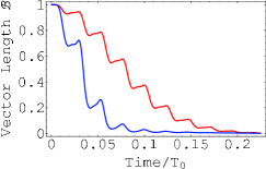
(b)

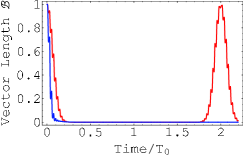
Figure 7: Plots of the qubit state Bloch vector length ${\mathcal{B}}(t)$ versus time for the decoherence free case (shown in red) and according to the irreversible bias current model (shown in blue). The time scale is parameterised in terms of the diagonal Wigner function term maximum separation time $T_{0}$. Here we note that in the case of the decoherence free plot the qubit state is a pure state at time $2nT_{0}$ where $n$ is a positive integer.

VII.2 Decoherence Due to Thermal Fluctuations in the Current Source

The irreversible bias current model presented so far not only has a dephasing effect when the readout current pulse is applied to the Quantronium circuit but also during the presence of noise in the current source. Here we look at the decoherence that our model predicts during the qubit manipulation stage when the mean of the readout current source is zero but has white noise fluctuations due to thermal noise in the resistor network which is used in conjunction with the voltage source in the Quantronium experiment to implement the readout current pulsecottetThesis . In this regime we consider the full master equation that includes the irreversible bias current decoherence term

$$\overset{.}{\rho}=-\frac{i}{\hbar}\left[H,\rho\right]+\frac{iE_{b}}{\hbar}\left[\gamma,\rho\right]-\frac{\left|E_{b}\right|}{2\hbar}\left[\gamma,\left[\gamma,\rho\right]\right],$$

and we write this in the operator formstace:062308

$$\overset{.}{\rho}={\mathcal{L}}_{H}\left\{\rho\right\}+\epsilon_{a}{\mathcal{L}}_{a}\left\{\rho\right\}+\epsilon_{b}{\mathcal{L}}_{b}\left\{\rho\right\}$$ (66)

where

$${\mathcal{L}}_{H}\left\{\rho\right\}=-\frac{i}{\hbar}[H,\rho],$$ (67)

$$\epsilon_{a}{\mathcal{L}}_{a}\left\{\rho\right\}=\frac{iE_{b}}{\hbar}[\gamma,\rho],$$ (68)

and

$$\epsilon_{b}{\mathcal{L}}_{b}\left\{\rho\right\}=-\frac{|E_{b}|}{2\hbar}[\gamma,\left[\gamma,\rho\right]].$$

Here $\epsilon_{a}$ and $\epsilon_{b}$ are small parameters compared to the qubit Hamiltonian $H$ and they are determined by the zero-bias current noise where $\epsilon_{a}=E_{b}$ and $\epsilon_{b}=|E_{b}|$. We assume $E_{b}$ fluctuates due to thermal noise in the external circuit, having zero mean. Therefore $E_{b}$ denotes the time fluctuating and zero mean current noise. For statistical purposes we treat $\epsilon_{a}$ and $\epsilon_{b}$ as independent variables. Since $\langle\epsilon_{b}\rangle=\langle|E_{b}|\rangle\neq 0$, we ignore fluctuations in $|E_{b}|$, whilst $\langle\epsilon_{a}\rangle=\langle E_{b}\rangle=0$ and so we consider the effect of thermal fluctuations in $E_{b}$. We write the solution to Eq. (66) as a correction to the exact solution $\rho_{0}$ of the noise free master equation

$$\overset{.}{\rho_{0}}=-\frac{i}{\hbar}\left[H,\rho_{0}\right],$$

that is, we can write the solution in the form $\rho=\rho_{0}+\epsilon_{a}\rho_{a}+\epsilon_{b}\rho_{b}+O(\epsilon^{2})$. That is, $\rho_{a}$ and $\rho_{b}$ represent the change of the density matrix due to the effect of fluctuations in the coherent term and for the intrinsic dissipative term (that depends on $|E_{b}|$) respectively. Substituting this solution $\rho$ into Eq. (66) and expanding the master equation to $O(\epsilon_{a})$ and $O(\epsilon_{b})$ gives

$$\overset{.}{\rho}_{0}={\mathcal{L}}_{H}\rho_{0},$$ (69)

$$\overset{.}{\rho}_{a}={\mathcal{L}}_{H}\rho_{a}+{\mathcal{L}}_{a}\rho_{0},$$ (70)

$$\overset{.}{\rho}_{b}={\mathcal{L}}_{H}\rho_{b}+{\mathcal{L}}_{b}\rho_{0}.$$ (71)

Defining $\widetilde{\rho}_{a}=\rho_{0}+\epsilon_{a}\rho_{a}$ and $\widetilde{\rho}_{b}=\rho_{0}+\epsilon_{b}\rho_{b}$ we find

$$\overset{.}{\widetilde{\rho}}_{a}=-\frac{i}{\hbar}[H,\widetilde{\rho}_{a}]+\frac{iE_{b}}{\hbar}[\gamma,\widetilde{\rho}_{a}]$$ (72)

and

$$\overset{.}{\widetilde{\rho}}_{b}=-\frac{i}{\hbar}\left[H,\widetilde{\rho}_{b}\right]-\frac{|E_{b}|}{2\hbar}\left[\gamma,\left[\gamma,\widetilde{\rho}_{b}\right]\right]$$ (73)

This allows us to treat the intrinsic dephasing of the current source and the dephasing due to thermal fluctuations in the washboard potential independently. Since $E_{b}$ fluctuates, the second term of Eq. (72) results in extra decoherence, on top of the intrinsic decoherence due to current passing through the readout Josephson junction described by Eq. (73). From these equations we can estimate the magnitude arising from these different effects.

Assuming the thermal fluctuations of $E_{b}$ are well approximated by white noise with zero mean we derive a master equation from Eq. (72) which describes the dephasing effect of a fluctuating current. By integrating Eq. (72) and substituting into the original master equation we have

$$\overset{.}{\widetilde{\rho}}_{a}= -\frac{i}{\hbar}\left[H,\widetilde{\rho}_{a}\right]$$

$$+\frac{i}{\hbar}\left[E_{b}(t)\gamma,-\frac{i}{\hbar}\int_{0}^{t}ds\left[H-E_{b}(s)\gamma,\widetilde{\rho}_{a}(s)\right]\right].$$ (74)

Taking the ensemble average of this equation and using $\langle E_{b}(t)\rangle=0$ and $\langle E_{b}(t)E_{b}(s)\rho(s)\rangle=\langle E_{b}(t)E_{b}(s)\rangle\langle\rho(s)\rangle$ (since $\langle\rho(t)\rangle$ is independent of future noise fluctuations) then

$$\langle\overset{.}{\widetilde{\rho}}_{a}\rangle= -\frac{i}{\hbar}\left[H,\left\langle\widetilde{\rho}_{a}\right\rangle\right]$$

$$-\frac{1}{\hbar^{2}}\int_{0}^{t}ds\left\langle E_{b}(t)E_{b}(s)\right\rangle\left[\gamma,\left[\gamma,\left\langle\widetilde{\rho}_{a}(s)\right\rangle\right]\right].$$

The noise correlation function satisfies

$$\left\langle E_{b}(t)E_{b}(s)\right\rangle= \left(\frac{\Phi_{0}}{2\pi}\right)^{2}\left\langle I_{bias}(t)I_{bias}(s)\right\rangle$$

$$= \left(\frac{\Phi_{0}}{2\pi}\right)^{2}{S_{I}}^{2}(0)\delta(t-s),$$

where by definition

$${S_{I}}^{2}(\omega)=\frac{1}{2\pi}\int_{-\infty}^{+\infty}e^{i\omega t}\left\langle I_{bias}(t)I_{bias}(0)\right\rangle dt$$

is the noise spectrum of the current fluctuations due to thermal noise. Thus, in the presence of noise, the master equation is of the form of Eq. (73). That is, it can be written as

$$\langle\overset{.}{\widetilde{\rho}}_{a}\rangle=-\frac{i}{\hbar}\left[H,\left\langle\widetilde{\rho}_{a}\right\rangle\right]-\left(\frac{S_{I}(0)\Phi_{0}}{2\pi\hbar}\right)^{2}\left[\gamma,\left[\gamma,\left\langle\widetilde{\rho}_{a}\right\rangle\right]\right].$$

Now for the Quantronium circuit with a current source output resistance $R_{1}$ at temperature $T$ and an effective input resistance of $R_{2}$, the current noise spectrum in terms of the thermal voltage noise spectrumnyquist $S_{V}(\omega)$ is

$$S_{I}(0)=\frac{S_{V}(0)}{R_{2}}=\frac{\sqrt{4R_{1}k_{b}T}}{R_{2}}.$$ (75)

The ensemble average of Eq. (73) is

$$\langle\overset{.}{\widetilde{\rho}}_{b}\rangle=-\frac{i}{\hbar}\left[H,\left\langle\widetilde{\rho}_{b}\right\rangle\right]-\frac{\left\langle\left|I_{bias}\right|\right\rangle\Phi_{0}}{4\pi\hbar}\left[\gamma,\left[\gamma,\left\langle\widetilde{\rho}_{b}\right\rangle\right]\right],$$

which establishes that the two kinds of dephasing have the same form. The rates due to the intrinsic dephasing of the current source and noise in the washboard potential are given by $\gamma_{deph}=\left\langle\left|I_{bias}\right|\right\rangle\Phi_{0}/(4\pi\hbar)$ and $\gamma_{noise}=(S_{I}(0)\Phi_{0}/(2\pi\hbar))^{2}$ respectively. We have so far assumed that $E_{b}$ is $\delta$-correlated. Under this white noise assumption $\langle|E_{b}|\rangle$ is singular so instead we estimate it from $I_{\textup{RMS}}$. The thermal noise in the current source is a result of the random scattering of electrons in the output resistance and this produces a statistical distribution of phonons in the phonon modes of the resistor. In the thermal state each phonon mode has a Gaussian distribution for the resultant voltage and hence current fluctuations. Summing over the phonon mode distributions in the resistor we obtain the total current fluctuations which is also Gaussian distributed. For Gaussian processes

$$\left\langle\left|I_{bias}\right|\right\rangle=\sqrt{\frac{2}{\pi}}I_{\textup{RMS}}.$$

and therefore we have

$$I_{\textup{RMS}}=\sqrt{\left\langle{I_{bias}}^{2}\right\rangle}=\frac{\sqrt{4R_{1}k_{b}TB}}{R_{2}}$$

where $B$ is the bandwidth of the Quantronium circuit.

We can now compare the sizes of the two dephasing terms by referring to the details of the Quantronium experimentcottetThesis . Analysing the readout circuit we can see that the thermal noise is produced by a $10\operatorname{k\Omega}$ resistor in series and a $50\Omega$ resistor in parallel with an ideal voltage source at the temperature of the helium bath. Also the thermal noise from these two resistors contribute to the fluctuating current that flows into the Quantronium Circuit via a $3.5\operatorname{k\Omega}$ input resistance which has a $200\operatorname{MHz}$ bandwidth. From these parameters we are able to determine that

$$\gamma_{noise}=\left(\frac{S_{I}(0)\Phi_{0}}{2\pi\hbar}\right)^{2}=9.68\operatorname{GHz}$$

and

$$\gamma_{deph}=\frac{\left\langle|I_{bias}|\right\rangle\Phi_{0}}{4\pi\hbar}=\frac{I_{\textup{RMS}}\Phi_{0}}{\sqrt{8\pi^{3}}\hbar}=555\operatorname{MHz},$$

meaning that the dephasing rate intrinsic to the irreversible bias current is about 20 times slower than the rate due to fluctuations in the titled washboard potential. From the relative scale of these two terms we can see that the dephasing during the qubit operation will be dominated by the fluctuations in the washboard potential, rather than the intrinsic irreversible bias current induced dephasing. However, we note that the introduction of the irreversible current source into the modelling process has still provided a dephasing effect of considerable size relative to the effect of thermal noise in the current source in this case, and therefore may be important for the consideration of other similar current biased superconducting circuit experimental models.

VIII Discussion and Conclusion

In this paper we have analysed the bias current readout process of the superconducting qubit structures such as the Quantronium (and by analogy those qubits whose quantum state is measured by a DC-SQUID like the persistent current qubit). By introducing an irreversible bias current term through Lindblad operators that describe the addition and subtraction of electrons across the readout Josephson junction, at a rate given by the bias current, we are able to obtain a master equation that can be approximated to first order by the Hamiltonian washboard potential model - a model that is used throughout the superconducting quantum device literature. Therefore this master equation incorporates an additional term to the washboard potential terms that dictate the decoherence of the qubit through its coupling to the readout Josephson junction.

The decoherence is a result of the bias current ‘counting’ the number of electrons that pass through the measurement Josephson junction. We propose that such an effect is intrinsic to the application of the bias current to the system and has a cumulative effect of decohering the system as electrons pass through the readout Josephson junction. By approximating the Hamiltonian terms by a harmonic oscillator coupled to a qubit in the symmetric superposition state were are able to analyse the measurement induced decoherence before a tunnelling process out of the washboard potential occurs and produces a measurable voltage for the experimentalist. Looking at this model in terms of the Quantronium experiment we have been able to construct the Wigner function for the Josephson junction and analyse the dephasing effect upon the application of the external bias current.

By analysing the Quantronium system we have found that the effect of describing the readout bias current in terms of the Lindblad operators is to produce a qubit dephasing time of 0.2 nanoseconds after the bias current has been applied. In the Quantronium experiment the bias current pulse was applied for a duration of the order of 0.1 microseconds, meaning that the state of the qubit has been reduced to a mixed state before the the tunnelling event from the washboard potential is observed. Our model changes the understanding of the measurement process of the Quantronium qubit and it means that the point of measurement is not the tunnelling event out of the washboard potential but instead arises as a consequence of coupling a current biased Josephson junction to the qubit state. Additionally this model does not produce extra sensitivity to noise in the current source since by adding thermal noise to the irreversible bias current model we showed that thermal noise in the washboard potential produces the dominant dephasing effect by an order of magnitude.

Experimental validation of our model could be predicted by using small current pulses during the Ramsey fringe experiment demonstrated by Vion et al. Vion since the role of the irreversible bias current is to dephase the qubit. Small amplitude and short duration current pulses could be applied to the Quantronium between $\pi/2$ pulses of a Ramsey fringe experiment. Our model would predict that for larger current and longer duration pulses the dephasing would become larger and hence influence the decay time seen in the Ramsey fringes. In addition to this the process shown in this paper of adding the irreversible bias current to the current biased Josephson junction qubitsXLiScience301-809 ; Martinis could be employed to look at the effect of the constant current through the Josephson junction and its resulting decoherence. In this case due to the utilisation of excited states of the washboard potential for the qubit states and readout, an appropriate replacement to the harmonic oscillator used in this paper would need to be employed.

IX Acknowledgements

We acknowledge fruitful discussions with H. S. Goan and C. A. C. Schelpe. GDH acknowledges the financial support of the Australian Research Council Special Research Centre for Quantum Computer Technology, Churchill College and the Cambridge Commonwealth Trust. This work was supported by the EPSRC and DTI under a Foresight LINK project.

Appendix A Analytical Calculation of the Off-Diagonal Wigner Function with Reversible Current Source

Using the commutation relation $[\gamma,N]=i$ which gives $e^{-i\theta N}|\gamma\rangle=|\gamma+\theta\rangle$ and the definition of the Wigner function

$$W(\alpha,\alpha^{*})=\int_{-\infty}^{+\infty}e^{\eta^{*}\alpha-\eta\alpha^{*}}\mathrm{Tr}\left\{\rho e^{\eta a^{\dagger}-\eta^{*}a}\right\}d^{2}\eta,$$

we can write

$$W(\gamma,N)=\frac{2}{\pi}\int_{-\infty}^{+\infty}e^{i\eta_{x}N}\left\langle\gamma-\eta_{x}/2|\rho|\gamma+\eta_{x}/2\right\rangle d\eta_{x}.$$ (76)

Using this form we can calculate the off-diagonal Wigner function $W_{\times}(\gamma,N)$ that corresponds to the density matrix component $\rho_{\times}(t)$ when we decompose the combined qubit and detector density matrix into the form:

$$\rho(t)= \rho_{+}(t)\left|0\right\rangle\left\langle 0\right|+\rho_{-}(t)\left|1\right\rangle\left\langle 1\right|$$

$$+\rho_{\times}(t)\left|0\right\rangle\left\langle 1\right|+{\rho_{\times}}^{\dagger}(t)\left|1\right\rangle\left\langle 0\right|.$$

We are able to calculate the off-diagonal Wigner function $W_{\times}(\gamma,N)$ in terms of the wavefunctions $|\psi_{0}(t)\rangle$ and $|\psi_{1}(t)\rangle$ which correspond to the single mode Gaussian wavefunctions of the Hamiltonian $H_{R}$ in the qubit eigenstates $|0\rangle$ and $|1\rangle$ respectively since

$$\rho_{\times}(t)=|\psi_{0}(t)\rangle\langle\psi_{1}(t)|.$$

The wavefunctions $|\psi_{0}(t)\rangle$ and $|\psi_{1}(t)\rangle$ evolve according to the Hamiltonians $H_{R+}$ and $H_{R-}$ respectively where

$$H_{R\pm}=\hbar\omega a^{\dagger}a\pm\hbar\chi\left(a+a^{\dagger}\right)^{2}+\hbar\epsilon\left(a+a^{\dagger}\right).$$

The $\gamma$ space wave function for the most general single mode Gaussian pure state is

$$\left\langle\gamma\big{|}\psi(t)\right\rangle= \left(2\pi\left\langle\left(\Delta\gamma\right)^{2}\right\rangle\right)^{-1}\exp(i\delta_{\gamma}/2)\exp(-iN_{0}\gamma_{0}/2)$$

$$\times\exp(iN_{0}\gamma)\exp(-\sigma\left(\gamma-\gamma_{0}\right)^{2}/2)$$ (77)

where

$$\gamma_{0}=\left\langle\gamma\right\rangle,$$

$$N_{0}=\left\langle N\right\rangle,$$

$$\sigma=\sigma_{1}+i\sigma_{2},$$

$$\sigma_{1}=\frac{1}{2\left\langle\left(\Delta\gamma\right)^{2}\right\rangle}$$

and

$$\sigma_{2}=-\frac{\langle\Delta\gamma\Delta N\rangle_{\mathrm{sym}}}{2\langle(\Delta\gamma)^{2}\rangle}=-\frac{\langle N\gamma\rangle+\langle\gamma N\rangle-2\langle\gamma\rangle\langle N\rangle}{2\langle(\Delta\gamma)^{2}\rangle}.$$

The phase angle $\delta_{\gamma}$ is set to zero. By using the single mode Gaussian form Eq. (77) and the Wigner function definition Eq. (76) we can calculate the off-diagonal Wigner function

$$W_{\times}(\gamma,N)=\frac{2}{\pi}\int_{-\infty}^{+\infty}e^{i\eta_{x}N}\left\langle\gamma-\frac{\eta_{x}}{2}\right|\rho_{\times}\left|\gamma+\frac{\eta_{x}}{2}\right\rangle d\eta_{x}$$

$$=\frac{2}{\pi}\int_{-\infty}^{+\infty}e^{i\eta_{x}N}\left\langle\gamma-\frac{\eta_{x}}{2}\Big{|}\psi_{0}\left(t\right)\right\rangle\left\langle\psi_{1}(t)\Big{|}\gamma+\frac{\eta_{x}}{2}\right\rangle d\eta_{x}.$$

This integral is in the form

$$\frac{C}{\sqrt{2\pi}}\int_{-\infty}^{+\infty}\mathrm{d}x~{}{e}^{\Theta x}{e}^{-\frac{1}{2}\Delta x^{2}}=\frac{1}{\sqrt{\Delta}}\exp{\frac{\Theta^{2}}{2\Delta}}$$

where

$$\Theta=iN-\frac{i}{2}(\langle N\rangle_{\scriptscriptstyle+}+\langle N\rangle_{\scriptscriptstyle-})$$

$$+\frac{1}{2}\sigma_{\scriptscriptstyle+}(\gamma-\langle\gamma\rangle_{\scriptscriptstyle+})-\frac{1}{2}{\sigma_{\scriptscriptstyle-}^{*}}(\gamma-\langle\gamma\rangle_{\scriptscriptstyle-}),$$

$$\Delta=\frac{1}{4}\sigma_{\scriptscriptstyle+}+\frac{1}{4}{\sigma_{\scriptscriptstyle-}^{*}}$$

and

$$C=\frac{2}{\pi\sqrt[4]{\langle(\Delta\gamma)^{2}\rangle_{\scriptscriptstyle+}\langle(\Delta\gamma)^{2}\rangle_{\scriptscriptstyle-}}}$$

$$\times\exp{\left(\frac{i}{2}(\langle N\rangle_{\scriptscriptstyle+}\langle\gamma\rangle_{\scriptscriptstyle+}-\langle N\rangle_{\scriptscriptstyle-}\langle\gamma\rangle_{\scriptscriptstyle-})+i\langle N\rangle_{\scriptscriptstyle+}\gamma-i\langle N\rangle_{\scriptscriptstyle-}\gamma\right)}$$

$$\times\exp{\left(-\frac{1}{2}\sigma_{\scriptscriptstyle+}(\gamma-\langle\gamma\rangle_{\scriptscriptstyle+})^{2}-\frac{1}{2}{\sigma_{\scriptscriptstyle-}}^{*}(\gamma-\langle\gamma\rangle_{\scriptscriptstyle-})^{2}\right)}.$$

Here we have used the notation $\langle\gamma\rangle_{\scriptscriptstyle\pm}$, $\langle N\rangle_{\scriptscriptstyle\pm}$, $\langle(\Delta\gamma)^{2}\rangle_{\scriptscriptstyle\pm}$ and $\sigma_{\scriptscriptstyle\pm}$ to distinguish the mean and noise parameters of the single mode Gaussian states $|\psi_{0}(t)\rangle$ and $|\psi_{1}(t)\rangle$ respectively.

In order to fully specify the off-diagonal Wigner function we need to calculate the quantities $\langle\gamma\rangle$, $\langle N\rangle$, $\sigma$ and $\delta_{x}$ for both the states $|\psi_{0}(t)\rangle$ and $|\psi_{1}(t)\rangle$ where

$$\langle\gamma\rangle=\sqrt{\frac{\lambda}{2}}(\langle a\rangle+\langle a^{\dagger}\rangle)$$

$$\langle N\rangle=-\frac{i}{\sqrt{2\lambda}}(\langle a\rangle-\langle a^{\dagger}\rangle)$$

$$\langle(\Delta\gamma)^{2}\rangle= \frac{\lambda}{2}(\langle aa\rangle+\langle a^{\dagger}a^{\dagger}\rangle+\langle aa^{\dagger}\rangle+\langle a^{\dagger}a\rangle$$

$$-2\langle a\rangle\langle a^{\dagger}\rangle-\langle a\rangle^{2}-\langle a^{\dagger}\rangle^{2})$$

and

$$\langle\Delta\gamma\Delta N\rangle_{\mathrm{sym}}= \langle N\gamma\rangle+\langle\gamma N\rangle-2\langle\gamma\rangle\langle N\rangle$$

$$= \frac{i}{2}(\langle a^{\dagger}a^{\dagger}\rangle-\langle aa\rangle+\langle a\rangle\langle a\rangle-\langle a^{\dagger}\rangle\langle a^{\dagger}\rangle).$$

To calculate these quantities we find the two sets of equations that solve for $\langle aa\rangle$, $\langle a^{\dagger}a^{\dagger}\rangle$, $\langle a^{\dagger}a\rangle$, $\langle aa^{\dagger}\rangle$, $\langle a\rangle$ and $\langle a^{\dagger}\rangle$ for the two qubit-eigenstate Hamiltonians for the system qubit and detector $H_{R\pm}$ in the qubit states $|0\rangle$ and $|1\rangle$ respectively. In order to find these we construct the set of six Heisenberg equations of motion for each Hamiltonian using the relation

$$dA/dt=-i[A,H_{R\pm}]/\hbar$$ (78)

and solve them simultaneously. From our Hamiltonians $H_{R+}$ and $H_{R-}$ respectively we find the set of two coupled differential equations

$${{d}\langle a\rangle}/{{d}t}= -i\omega\langle a\rangle\mp 2i\chi(\langle a^{\dagger}\rangle+\langle a\rangle)-i\epsilon$$

$${{d}\langle a^{\dagger}\rangle}/{\mathrm{d}t}= +i\omega\langle a^{\dagger}\rangle\pm 2i\chi(\langle a^{\dagger}\rangle+\langle a\rangle)+i\epsilon,$$

which we solve using the initial conditions $\langle a(0)\rangle=0$ and $\langle a^{\dagger}(0)\rangle=0$. The four remaining, coupled equations of motion for $H_{R+}$ and $H_{R-}$ are

$${{d}\langle aa\rangle}/{{d}t}= -2i\left(\omega\pm 2\chi\right)\langle aa\rangle$$

$$\mp 2i\chi(\langle a^{\dagger}a\rangle+\langle aa^{\dagger}\rangle)-2i\epsilon\langle a\rangle$$

$${{d}\langle a^{\dagger}a^{\dagger}\rangle}/{{d}t}= +2i\left(\omega\pm 2\chi\right)\langle a^{\dagger}a^{\dagger}\rangle$$

$$\pm 2i\chi(\langle a^{\dagger}a\rangle+\langle aa^{\dagger}\rangle)+2i\epsilon\langle a^{\dagger}\rangle$$

$${{d}\langle a^{\dagger}a\rangle}/{{d}t}= \mp 2i\chi(\langle a^{\dagger}a^{\dagger}\rangle-\langle aa\rangle)-i\epsilon(\langle a^{\dagger}\rangle-\langle a\rangle)$$

$${{d}\langle aa^{\dagger}\rangle}/{{d}t}= \mp 2i\chi(\langle a^{\dagger}a^{\dagger}\rangle-\langle aa\rangle)-i\epsilon(\langle a^{\dagger}\rangle-\langle a\rangle),$$

Using the solutions $\langle a\rangle_{t}$ and $\langle a^{\dagger}\rangle_{t}$ we write the four coupled differential equations in matrix form $\nabla_{t}=A.x+v$, where $x=(aa,a^{\dagger}a^{\dagger},a^{\dagger}a,aa^{\dagger},a^{\dagger},a)^{T}$, $\nabla_{t}$ contains the time derivatives of the components of $x$, and $v$ contains the terms containing $\langle a\rangle_{t}$ and $\langle a^{\dagger}\rangle_{t}$. We solve this system of equations by diagonalising the matrix $A$ by forming the matrix $D$ containing its eigenvectors corresponding to the eigenvalues

$$\left\{0,0,+2i\sqrt{\omega^{2}\pm 4\omega\chi},-2i\sqrt{\omega^{2}\pm 4\omega\chi}\right\}.$$

Once in the diagonal form $D^{-1}.\nabla_{t}=D^{-1}A.D.D^{-1}.x+D^{-1}.v$ we can solve the four uncoupled differential equations and then transform back the solution to the original basis. Using the initial conditions $\langle aa\rangle_{0}=0,\langle a^{\dagger}a^{\dagger}\rangle_{0}=0,\langle a^{\dagger}a\rangle_{0}=0,\langle aa^{\dagger}\rangle_{0}=0$ and $\langle a^{\dagger}a\rangle_{0}=1$ we have the solution for $\gamma_{0}$, $N_{0}$ and $\sigma$:

$$\langle\gamma\rangle_{\pm}=\frac{\sqrt{2\lambda}\epsilon(\cos{(t\sqrt{\omega^{2}\pm 4\omega\chi})}-1)}{\omega\pm 4\chi}$$

$$\langle N\rangle_{\pm}=-\frac{\sqrt{2}\epsilon\sin{(t\sqrt{\omega^{2}\pm 4\omega\chi})}}{\sqrt{\lambda(\omega^{2}\pm 4\omega\chi)}}$$

$$\sigma_{\pm}=\frac{\omega^{2}\pm 2\chi(2\omega+i\sqrt{\omega^{2}\pm 4\omega\chi}\sin{(2t\sqrt{\omega^{2}\pm 4\omega\chi}))}}{\lambda\omega(\omega\pm 2\chi(1+\cos{(2t\sqrt{\omega^{2}\pm 4\omega\chi}))})}$$

$$\langle(\Delta\gamma)^{2}\rangle_{\pm}=\frac{\lambda(\omega\pm 2\chi(1+\cos{(2t\sqrt{\omega^{2}\pm 4\omega\chi}))})}{2(\omega\pm 4\chi)}$$

In this calculation we have set the phase angle $\delta_{\gamma}$ to zero for both the $|\psi_{0}(t)\rangle$ and $|\psi_{1}(t)\rangle$ states. Now that we have fully specified the mean and noise parameters for the two single mode Gaussian sates $|\psi_{0}(t)\rangle$ and $|\psi_{1}(t)\rangle$ we can write this solution in the form $W_{\times}(\gamma,N)=\exp(a(t)\gamma+b(t)N+c(t)\gamma^{2}+d(t)\gamma N+e(t)N^{2}+f(t))$ where

$$a(t)=\frac{(i\langle N\rangle_{\scriptscriptstyle+}+i\langle N\rangle_{\scriptscriptstyle-}+\sigma_{\scriptscriptstyle+}\langle\gamma\rangle_{\scriptscriptstyle+}-\sigma_{\scriptscriptstyle-}^{*}\langle\gamma\rangle_{\scriptscriptstyle-})(\sigma_{\scriptscriptstyle-}^{*}-\sigma_{\scriptscriptstyle+})}{\sigma_{\scriptscriptstyle+}+{\sigma_{\scriptscriptstyle-}^{*}}}$$

$$+i\langle N\rangle_{\scriptscriptstyle+}-i\langle N\rangle_{\scriptscriptstyle-}+\sigma_{\scriptscriptstyle+}\langle\gamma\rangle_{\scriptscriptstyle+}+{\sigma_{\scriptscriptstyle-}^{*}}\langle\gamma\rangle_{\scriptscriptstyle-}$$

$$b(t)=\frac{2(\langle N\rangle_{\scriptscriptstyle+}+\langle N\rangle_{\scriptscriptstyle-})-2i\sigma_{\scriptscriptstyle+}\langle\gamma\rangle_{\scriptscriptstyle+}+2i{\sigma_{\scriptscriptstyle-}^{*}}\langle\gamma\rangle_{\scriptscriptstyle-}}{\sigma_{\scriptscriptstyle+}+{\sigma_{\scriptscriptstyle-}^{*}}}$$

$$c(t)=-\frac{1}{2}\sigma_{\scriptscriptstyle+}-\frac{1}{2}{\sigma_{\scriptscriptstyle-}^{*}}+\frac{(\sigma_{\scriptscriptstyle+}-{\sigma_{\scriptscriptstyle-}^{*}})^{2}}{2(\sigma_{\scriptscriptstyle+}+{\sigma_{\scriptscriptstyle-}^{*}})}$$

$$d(t)=\frac{2i{\sigma_{\scriptscriptstyle-}^{*}}-2i\sigma_{\scriptscriptstyle+}}{\sigma_{\scriptscriptstyle+}+{\sigma_{\scriptscriptstyle-}^{*}}}$$

$$e(t)=-\frac{2}{\sigma_{\scriptscriptstyle+}+{\sigma_{\scriptscriptstyle-}^{*}}}$$

and

$$f(t)=\ln{\left(\frac{4}{\pi\sqrt{\sigma_{\scriptscriptstyle+}+{\sigma_{\scriptscriptstyle-}^{*}}}\sqrt[4]{\langle(\Delta\gamma)^{2}\rangle_{\scriptscriptstyle+}\langle(\Delta\gamma)^{2}\rangle_{\scriptscriptstyle-}}}\right)}$$

$$+\frac{i}{2}(\langle N\rangle_{\scriptscriptstyle+}\langle\gamma\rangle_{\scriptscriptstyle+}-\langle N\rangle_{\scriptscriptstyle-}\langle\gamma\rangle_{\scriptscriptstyle-})$$

$$-\frac{1}{2}\sigma_{\scriptscriptstyle+}{\langle\gamma\rangle_{\scriptscriptstyle+}}^{2}-\frac{1}{2}{\sigma_{\scriptscriptstyle-}^{*}}{\langle\gamma\rangle_{\scriptscriptstyle-}}^{2}$$

$$+\frac{(i\langle N\rangle_{\scriptscriptstyle+}+i\langle N\rangle_{\scriptscriptstyle-}+\sigma_{\scriptscriptstyle+}\langle\gamma\rangle_{\scriptscriptstyle+}-\sigma_{\scriptscriptstyle-}^{*}\langle\gamma\rangle_{\scriptscriptstyle-})^{2}}{2(\sigma_{\scriptscriptstyle+}+{\sigma_{\scriptscriptstyle-}^{*}})}$$

Appendix B Analytical Calculation of the Off-Diagonal Wigner Function with Irreversible Current Source

For the off-diagonal term $W_{\times}(\gamma,N)$ of the Wigner function including measurement induced decoherence we solve (Eq. (48)) with a solution in the non-positive definite form

$$W_{\times}(\gamma,N,t)=\exp( a(t)\gamma+b(t)N+c(t)\gamma^{2}$$

$$+d(t)\gamma N+e(t)N^{2}+f(t)).$$

Using this form of solution we can derive the set of six coupled differential equations:

$$\overset{.}{a}(t) =\frac{\omega}{\lambda_{\times}}b(t)+Gd(t)+\frac{\left(-I+iE\right)}{2}b(t)d(t),$$

$$\overset{.}{b}(t) =-\lambda_{\times}\omega a(t)+2Ge(t)+\left(-I+iE\right)e(t)b(t),$$

$$\overset{.}{c}(t) =\frac{\omega}{\lambda_{\times}}d(t)-iE+\frac{\left(-I+iE\right)}{4}d(t)^{2},$$

$$\overset{.}{d}(t) =-2\lambda_{\times}\omega c(t)+\frac{2\omega}{\lambda_{\times}}e(t)+\left(-I+iE\right)e(t)d(t),$$

$$\overset{.}{e}(t) =-\lambda_{\times}\omega d(t)+\left(-I+iE\right)e(t)^{2},$$

$$\overset{.}{f}(t) =Gb(t)+\frac{\left(-I+iE\right)}{4}\left(2e(t)+b(t)^{2}\right),$$

where $G=-E_{b}/\hbar$, $I=-2|E_{b}|/\hbar$ and $E=E_{J}/4\hbar$. This system of equations is solved by first considering the three coupled equations for $\overset{.}{c}(t)$, $\overset{.}{d}(t)$ and $\overset{.}{e}(t)$ whereby using the transformation of variables

$$z=\frac{d+i(\frac{c}{\lambda_{\times}}-\lambda_{\times}e)}{4i},$$

$$\bar{z}=\frac{d-i(\frac{c}{\lambda_{\times}}-\lambda_{\times}e)}{4i},$$

and

$$u=\frac{(\frac{c}{\lambda_{\times}}+\lambda_{\times}e)}{4}$$

we have

$$\overset{.}{z}=2i\omega_{\times}z-\left(-I+iE\right)\left(z-u\right)^{2}/2-2iE,$$

$$\overset{.}{\overset{\_}{z}}=-2i\omega_{\times}\overset{\_}{z}+\left(-I+iE\right)\left(\overset{\_}{z}+u\right)^{2}/2+2iE,$$

$$\overset{.}{u}=-\left(-I+iE\right)\left(z-u\right)\left(\overset{\_}{z}+u\right)/2-2iE.$$

Using the relation $dZ/dt=-(-I+iE)Z(z-\overset{\_}{z}-2u)$, where $Z=z\overset{\_}{z}+u^{2}-iE/(-I+iE)$, we use a second transformation of variables

$$U=u/Z,$$

$$A=z/Z$$

and

$$\overset{\_}{A}=\overset{\_}{z}/Z$$

so that

$$\overset{.}{U}=-\frac{\left(-I+iE\right)}{2}\frac{\left(z\overset{\_}{z}+u^{2}+4iE/\left(-I+iE\right)\right)}{\left(z\overset{\_}{z}+u^{2}-4iE/\left(-I+iE\right)\right)},$$

$$\overset{.}{A}=2i\omega_{\times}A-\frac{\left(-I+iE\right)}{2}\frac{\left(z\overset{\_}{z}+u^{2}+4iE/\left(-I+iE\right)\right)}{\left(z\overset{\_}{z}+u^{2}-4iE/\left(-I+iE\right)\right)},$$

$$\overset{.}{\overset{\_}{A}}=-2i\omega_{\times}A+\frac{\left(-I+iE\right)}{2}\frac{\left(z\overset{\_}{z}+u^{2}+4iE/\left(-I+iE\right)\right)}{\left(z\overset{\_}{z}+u^{2}-4iE/\left(-I+iE\right)\right)}.$$

From these equations we construct the differential equation

$$\frac{d^{4}P}{dt^{4}}+4\omega_{\times}^{2}\frac{d^{2}P}{dt^{2}}-16\omega_{\times}^{2}iE(-I+iE)P=0$$

where

$$P=\frac{\left(z\overset{\_}{z}+u^{2}+4iE/\left(-I+iE\right)\right)}{\left(z\overset{\_}{z}+u^{2}-4iE/\left(-I+iE\right)\right)}$$

The solution $P$ is the sum of exponentials

$$P=C_{1}e^{\lambda_{1}t}+C_{2}e^{-\lambda_{1}t}+C_{3}e^{\lambda_{2}t}+C_{4}e^{-\lambda_{2}t}$$

where

$$\lambda_{1,2}=\sqrt{-2\omega_{\times}^{2}\pm 2\omega_{\times}\sqrt{\omega_{\times}^{2}-4{E^{2}}-4iEI}}$$

and

$$C_{1,2}=\frac{{\lambda_{2}}^{2}(2I-iE\pm E(E+4iI)/(2\lambda_{1})}{4I({\lambda_{2}}^{2}-{\lambda_{1}}^{2})},$$

$$C_{3,4}=-\frac{{\lambda_{1}}^{2}(2I-iE\pm E(E+4iI)/(2\lambda_{2})}{4I({\lambda_{2}}^{2}-{\lambda_{1}}^{2})}.$$

From $P$ we have the solutions for $c(t)$, $d(t)$ and $e(t)$

$$c(t)=\frac{(2w^{2}\frac{dP}{dt}+\frac{d^{2}P}{dt^{2}})}{4\lambda_{\times}w^{2}(-I+iE)(1-P)}$$

$$d(t)=-\frac{1}{2w(-I+iE)(1-P)}\frac{d^{2}P}{dt^{2}}$$

$$e(t)=\frac{\lambda_{\times}}{2(-I+iE)(1-P)}\frac{dP}{dt}.$$

If $I=0$, $\lambda_{1,2}$ are pure imaginary and so $P$ simply oscillates resulting in oscillatory solutions for $c(t)$, $d(t)$, $e(t)$. The remaining coeffcients $a(t)$ and $b(t)$ are coupled together, satisfying a forced, parametrically excited second order ordinary differential equation. To see this let

$$a(t) =\frac{i}{2(1-P(t))\sqrt{2\lambda_{\times}}}\frac{d(y(t)\sqrt{1-P(t)})}{dt}$$

$$b(t) =\sqrt{\frac{\lambda_{\times}}{2}}\left(-\frac{iy(t)}{2\sqrt{1-P(t)}}+\frac{4G}{(-I+iE)}\right).$$

Then $y(t)$ satifies the following equation.

$$\frac{d^{2}y}{dt^{2}}+\left(1-\frac{1}{2}\left(\frac{1}{(1-P(t))}\frac{dP(t)}{dt}\right)^{2}\right)y(t)=-\frac{4iG\sqrt{1-P(t)}}{-I+iE}$$

Since initially both $a(0)=0$ and $b(0)=0$ their subsequent solution is proportional to $G$ and

$$\frac{b^{2}(t)c(t)-a(t)b(t)d(t)+a^{2}(t)e(t)}{4c(t)e(t)-d^{2}(t)}$$

is proportional to $G^{2}$. Initially this is zero and for small times is quadratic in time. The solution to $f(t)$ is found through integration.

References

- (1) M. A. Nielsen and I. L. Chuang, Quantum Computation and Quantum Information (Cambridge University Press, Cambridge, 2000).
- (2) I. L. Chuang, L. M. Vandersypen, X. L. Zhou, D. W. Leung and S. Lloyd, Nature (London), 393, 143, (1998).
- (3) L. M. Vandersypen, M. Steffan, G. Breyta, C. S. Yannoni, M. H. Sherwood and I. L. Chuang, Nature (London), 414, 883, (2001).
- (4) C. A. Sackett, D. Kielpinski, B. E. King, C. Langer, V. Meyer, C. J. Myatt, M. Rowe, Q. A. Turchette, W. M. Itano, D. J. Wineland and C. Monroe, Nature (London), 404, 256, (2000).
- (5) D. Kielpinski, C. Monroe and D. J. Wineland, Nature, 417, 709, (2002).
- (6) E. Knill, R. Laflamme and G. J. Milburn, Nature (London), 409, 46, (2001).
- (7) J. L. O’Brien, G. J. Pryde, A. G. White, T. C. Ralph and D. Branning, Nature (London), 426, 264, (2003).
- (8) B. E. Kane, Nature (London), 393, 133, (1998).
- (9) R. H. Blick, D. Pfannkuche, R. J. Haug, K. v. Klitzing and K. Eberl, Phys. Rev. Lett., 80, 4032, (1998).
- (10) T. Hayashi, T. Fujisawa, H. D. Cheong, Y. H. Jeong and Y. Hirayama, Phys. Rev. Lett., 91, 226804, (2003).
- (11) T. H. Oosterkamp, T. Fujisawa, W. G. van der Wiel, K. Ishibashi, R. V. Hijman, S. Tarucha and L. P. Kouwenhoven, Nature, 395, 873, (1998).
- (12) X. Li, Y. Wu, D. Steel, D. Gammon, T. H. Stievater, D. S. Katzer, D. Park, C. Piermarocchi and L. J. Sham, Science, 301, 809, (2003).
- (13) Y. Makhlin, G. Schon and A. Shnirman, Rev. Mod. Phys., 73, 357, (2001).
- (14) Y. Nakamura, Y. A. Pashkin and J. S. Tsai, Nature (London), 398, 786, (1999).
- (15) J. M. Martinis, S. Nam, J. Aumentado and C. Urbina, Phys. Rev. Lett., 89, 117901, (2002).
- (16) Y. Yu, S. Han, X. Chu, S. Chu and Z. Wang, Science, 296, 889, (2002).
- (17) I. Chiorescu, Y. Nakamura, C. J. Harmans and J. E. Mooij, Science, 299, 1869, (2003).
- (18) D. Vion, A. Aassime, A. Cottet, P. Joyez, H. Pothier, C. Urbina, D. Esteve and M. H. Devoret, Science, 296, 886, (2002).
- (19) Y. A. Pashkin, T. Yamamoto, O. Astafiev, Y. Nakamura, D. V. Averin and J. S. Tsai, Nature (London), 421, 823, (2003).
- (20) A. J. Berkley, H. Xu, R. C. Ramos, M. A. Gubrud, F. W. Strauch, P. R. Johnson, J. R. Anderson, A. J. Dragt, C. J. Lobb and F. C. Wellstood, Science, 300, 1548, (2003).
- (21) G. Lindblad, Commun. Math. Phys., 48, 119, (1976).
- (22) A. O. Caldeira and A. J. Leggett, Ann. Phys. (N.Y.), 149, 374, (1983).
- (23) T. M. Stace and S. D. Barrett Phys. Rev. Lett., 92, 136802, (2004).
- (24) J. Tejada, E. M. Chudnovsky, E. d. Barco, J. M. Hernandez and T. P. Spiller, Nanotechnology, 12, 181, (2001).
- (25) M. Tinkham, Introduction to Superconductivity (McGraw-Hill, New York, 1996).
- (26) J. M. Martinis, M. H. Devoret and J. Clarke, Phys. Rev. B, 35, 4682, (1987).
- (27) J. M. Martinis, M. H. Devoret and J. Clarke, Phys. Rev. Lett., 55, 1543, (1985).
- (28) T. P. Spiller, T. D. Clark, H. Prance, R. J. Prance and J. F. Ralph, J. Low Temp. Phys., 5/6, 119, (1995).
- (29) P. Joyez, P. Lafarge, A. Filipe, D. Esteve and M. H. Devoret, Phys. Rev. Lett., 72, 2458, (1994).
- (30) A. Cottet, D. Vion, A. Aassime, P. Joyez, D. Esteve and M. H. Devoret, Physica C, 367, 197, (2002).
- (31) A. Cottet, Ph.D. thesis, L’Universitè Paris VI, 2002.
- (32) K. Hasselbach, C. Veauvy and D. Mailly, Physica C, 332, 140, (2000).
- (33) M. Hillery, R. F. O’Connell, M. O. Scully and E. P. Wigner, Physics Reports, 106, 121, (1984).
- (34) D. F. Walls and G. J. Milburn, Quantum Optics (Springer-Verlag, Berlin, 1995).
- (35) M. C. Wang and G. E. Uhlenback, Rev. Mod. Phys., 17, 323, (1945).
- (36) T. M. Stace and C. H. W. Barnes Phys. Rev. A, 65, 062308, (2002).
- (37) H. Nyquist Phys. Rev., 32, 110, (1928).