Simultaneous amplification and non-symmetric amplitude damping of two-mode Gaussian state

Abstract

The evolution of two-mode Gaussian state under symmetric amplification, non-symmetric damping and thermal noise is studied. The time dependent solution of the state characteristic function is obtained. The separability criterions are given for the final state of weak amplification as well as strong amplification.

PACS: 03.65.Yz ; 42.50.Dv; 42.50.Lc

Keywords: parametric amplifier, non-symmetric amplitude damping, separability, Gaussian state

1 Introduction

In all practical instances the information and entanglement contained in a given quantum state of the system, so precious for the realization of any specific task, is constantly threatened by the unavoidable interaction with the environment. Such an interaction entangles the system of interest with the environment, causing any amount of information to be scattered and lost in the environment. The overall process, corresponding to a non unitary evolution of the system, is commonly referred to as decoherence. To overcome the loss, parameter amplifier is added to the system. We in this paper will treat the simultaneous actions of amplitude damping and parameter amplification to two-mode Gaussian state.

The density matrix obeys the following master equation [1] $\frac{d\rho}{dt}=-\frac{i}{\hbar}[H,\rho]+\mathcal{L}\rho,$with the quadratic Hamiltonian $H=\hbar\sum_{jk}\frac{i}{2}(\eta_{jk}a_{j}^{\dagger}a_{k}^{\dagger}-\eta_{jk}^{*}a_{j}a_{k})$, where $\eta$ is a complex symmetric matrix (parameter amplifier matrix). $\mathcal{L}_{1}\rho=\sum_{j}\frac{\Gamma_{j}}{2}\{(\overline{n}_{j}+1)L[a_{j}]\rho+\overline{n}_{j}L[a_{j}^{\dagger}]\rho\},$where the Lindblad super-operators are defined as $L[\widehat{o}]\rho\equiv$ $2\widehat{o}\rho\widehat{o}^{\dagger}-\widehat{o}^{\dagger}\widehat{o}\rho-\rho\widehat{o}^{\dagger}\widehat{o}$ $,\Gamma_{j}$ is the amplitude damping coefficient of $jth$ mode, $\overline{n}_{j}$ is the average thermal photon number of the environment. Any quantum state can be equivalently specified by its characteristic function. Every operator $\mathcal{A}\in\mathcal{B(H)}$ is completely determined by its characteristic function $\chi_{\mathcal{A}}:=tr[\mathcal{AD}(\mu)]$ [2], where $\mathcal{D}(\mu)=\exp(\mu a^{\dagger}-\mu^{*}a)$ is the displacement operator, with $\mu=[\mu_{1},\mu_{2},\cdots,\mu_{s}]$ $,a=[a_{1},a_{2},\cdots,a_{s}]^{T}$ and the total number of modes is $s.$ It follows that $\mathcal{A}$ may be written in terms of $\chi_{\mathcal{A}}$ as [3]: $\mathcal{A}=\int[\prod_{i}\frac{d^{2}\mu_{i}}{\pi}]\chi_{\mathcal{A}}(\mu)\mathcal{D}(-\mu).$ The density matrix $\rho$ can be expressed with its characteristic function $\chi$. $\chi=tr[\rho\mathcal{D}(\mu)]$ . The master equation can be transformed to the diffusion equation of the characteristic function, it is [4] [5]

$$\frac{\partial\chi}{\partial t}=-\sum_{jk}(\eta_{jk}\mu_{j}^{*}\frac{\partial\chi}{\partial\mu_{k}}+\eta_{jk}^{*}\mu_{j}\frac{\partial\chi}{\partial\mu_{k}^{*}})-\frac{1}{2}\sum_{j}\Gamma_{j}\{\left|\mu_{j}\right|\frac{\partial\chi}{\partial\left|\mu_{j}\right|}+(2\overline{n}_{j}+1)\left|\mu_{j}\right|^{2}\chi\}.$$ (1)

2 The parametric amplifier and the amplitude damping

The solution of the diffusion equation of the characteristic function can be completely worked out for Gaussian state in the case of real parameter amplifier matrix $\eta$. We will consider real $\eta$ in the following. If the initial state is Gaussian, its characteristic function has the form of $\chi(\mu,\mu^{*},0)=\exp[\mu m^{\dagger}(0)-\mu^{*}m^{T}(0)-\frac{1}{2}(\mu,-\mu^{*})\gamma(0)(\mu^{*},-\mu)^{T}],$ the state will keep to be a Gaussian state in later evolution, where $m$ is the first moment and is irrelevant to entanglement, $\gamma$ is the complex correlation matrix (CM). The time evolution of the complex CM for real amplifier matrix $\eta$ is [5]

$$\gamma(t)=\left[\begin{array}[]{ll}M&-N\\ -N&M\end{array}\right](\gamma(0)-\left[\begin{array}[]{ll}\alpha&\beta^{*}\\ \beta&\alpha^{*}\end{array}\right])\left[\begin{array}[]{ll}M&-N\\ -N&M\end{array}\right]+\left[\begin{array}[]{ll}\alpha&\beta^{*}\\ \beta&\alpha^{*}\end{array}\right].$$ (2)

where $M$ and $N$ are the solutions of the following matrix equations $\frac{dM}{dt}=-\eta N-\frac{\Gamma}{2}M,\frac{dN}{dt}=-\eta M-\frac{\Gamma}{2}N,$with $\Gamma=diag\{\Gamma_{1},\Gamma_{2},\cdots,\Gamma_{s}\}.$ The solution is $M=\frac{1}{2}[\exp(-\eta t-\frac{\Gamma t}{2})+\exp(\eta t-\frac{\Gamma t}{2})],$ $N=\frac{1}{2}[\exp(-\eta t-\frac{\Gamma t}{2})-\exp(\eta t-\frac{\Gamma t}{2})].$ The constant matrices $\alpha$ and $\beta$ in 2 have the behaviors $\alpha^{\dagger}=\alpha,$ $\beta=\beta^{T}$, they are the solutions of the following matrix equations

$$2(\eta\alpha+\alpha^{*}\eta)-\Gamma\beta-\beta\Gamma = 0,$$ (3)

$$\Gamma\alpha+\alpha\Gamma-2\eta\beta-2\beta^{*}\eta-\Gamma(\overline{n}+\frac{1}{2})-(\overline{n}+\frac{1}{2})\Gamma = 0.$$ (4)

where $\overline{n}=diag\{\overline{n}_{1},\overline{n}_{2},\cdots,\overline{n}_{s}\}.$ The one mode solution has been known for a long time (see [6] and references therein).

For the two-mode situation, the real amplifier matrix $\eta=\eta_{0}\sigma_{0}+\eta_{1}\sigma_{1}+\eta_{3}\sigma_{3},$where $\sigma_{0}=I_{2},\sigma_{1},\sigma_{3}$ are Pauli matrices. $M$ and $N$ can be simplified to

$$M = \frac{1}{2}e^{-C_{1}t}[\cosh(B_{1}t)\sigma_{0}-\sinh(B_{1}t)\overrightarrow{\sigma}\cdot\overrightarrow{b_{1}}]+\frac{1}{2}e^{-C_{2}t}[\cosh(B_{2}t)\sigma_{0}-\sinh(B_{2}t)\overrightarrow{\sigma}\cdot\overrightarrow{b_{2}}],$$ (5)

$$N = \frac{1}{2}e^{-C_{1}t}[\cosh(B_{1}t)\sigma_{0}-\sinh(B_{1}t)\overrightarrow{\sigma}\cdot\overrightarrow{b_{1}}]-\frac{1}{2}e^{-C_{2}t}[\cosh(B_{2}t)\sigma_{0}-\sinh(B_{2}t)\overrightarrow{\sigma}\cdot\overrightarrow{b_{2}}].$$ (6)

where $C_{1,2}=\pm\eta_{0}+\frac{1}{4}(\Gamma_{1}+\Gamma_{2});$ $B_{1,2}=\sqrt{\eta_{1}^{2}+(\frac{1}{4}(\Gamma_{1}-\Gamma_{2})\pm\eta_{3})^{2}};$ $\overrightarrow{b}_{1,2}=(\pm\eta_{1},0,\pm\eta_{3}+\frac{1}{4}(\Gamma_{1}-\Gamma_{2}))/B_{1,2}.$ We will consider the case of symmetric noise, that is, $\overline{n}=\overline{n}_{0}\mathbf{I}_{2.}$The solutions of equations (3) and (4) are given in the appendix.

3 The inter-mode amplifier

The algebra equation of $\alpha$ and $\beta$ in two mode system is complicated in general situation. To investigate the entanglement property of the amplifier, we will first consider the case of $\eta_{0}=\eta_{3}=0$ which corresponds to inter-mode amplification alone. Thus $\eta=\eta_{1}\sigma$. The solution is (see Appendix)

$$\alpha = \frac{\overline{n}_{0}^{\prime}}{1-\Gamma_{3}^{\prime 2}-\eta_{1}^{\prime 2}}[(1-\Gamma_{3}^{\prime 2})\sigma_{0}+\Gamma_{3}^{\prime}\eta_{1}^{\prime 2}\sigma_{3}],$$ (7)

$$\beta = \frac{\overline{n}_{0}^{\prime}\eta_{1}^{\prime}(1-\Gamma_{3}^{\prime 2})}{1-\Gamma_{3}^{\prime 2}-\eta_{1}^{\prime 2}}\sigma_{1},$$ (8)

where $\overline{n}_{0}^{\prime}=\overline{n}_{0}+\frac{1}{2},$ $\Gamma_{3}^{{}^{\prime}}=\Gamma_{3}/\Gamma_{0},\eta_{1}^{\prime}=2\eta_{1}/\Gamma_{0}.$ In the assumption of $\eta_{0}=\eta_{3}=0,$ we have $C_{1}=C_{2}=\Gamma_{0}/2;$ $B_{1}=B_{2}=\sqrt{\left(\Gamma_{3}/2\right)^{2}+\eta_{1}^{2}}=k\Gamma_{0}/2$, with $k=\sqrt{\Gamma_{3}^{{}^{\prime}2}+\eta_{1}^{\prime 2}}.$ Denote $t^{\prime}=\Gamma_{0}t/2,$hence

$$M = e^{-t^{\prime}}[\cosh(kt^{\prime})\sigma_{0}-\sinh(kt^{\prime})\frac{\Gamma_{3}^{\prime}}{k}\sigma_{3}]$$ (9)

$$N = -e^{-t^{\prime}}\sinh(kt^{\prime})\frac{\eta_{1}^{\prime}}{k}\sigma_{1}$$ (10)

For the case of weak amplifier, $k<1$, that is , $\eta_{1}^{2}<\frac{1}{4}(\Gamma_{0}^{2}-\Gamma_{3}^{2}),$ when $t\rightarrow\infty,$ we have $M,N\rightarrow 0.$ The state will tend to a Gaussian state which is characterized by the residue complex CM $\gamma(\infty)$ $=\left[\begin{array}[]{ll}\alpha&\beta^{*}\\ \beta&\alpha^{*}\end{array}\right]$. The Peres-Horodecki criterion for separability [7] [8] will be [5]

$$\det\gamma_{a}\det\gamma_{b}+(\frac{1}{4}-\left|\det\gamma_{c}\right|)^{2}-tr(\gamma_{a}\sigma_{3}\gamma_{c}\sigma_{3}\gamma_{b}\sigma_{3}\gamma_{c}^{\dagger}\sigma_{3})\geq\frac{1}{4}(\det\gamma_{a}+\det\gamma_{b}),$$ (11)

where

$$\alpha=\left[\begin{array}[]{ll}\alpha_{a}&\alpha_{c}\\ \alpha_{c}^{*}&\alpha_{b}\end{array}\right],\text{ }\beta=\left[\begin{array}[]{ll}\beta_{a}&\beta_{c}\\ \beta_{c}&\beta_{b}\end{array}\right],\gamma_{i}^{\prime}=\left[\begin{array}[]{ll}\alpha_{i}&\beta_{i}^{*}\\ \beta_{i}&\alpha_{i}^{*}\end{array}\right],\text{ }i=a,b,c.$$ (12)

Then $\alpha_{a}=$ $\frac{\overline{n}_{0}^{\prime}}{1-k^{2}}(1-\Gamma_{3}^{\prime 2}+\Gamma_{3}^{\prime}\eta_{1}^{\prime 2}),$ $\alpha_{b}=\frac{\overline{n}_{0}^{\prime}}{1-k^{2}}(1-\Gamma_{3}^{\prime 2}-\Gamma_{3}^{\prime}\eta_{1}^{\prime 2}),$ $\alpha_{c}=0;$ $\beta_{c}=\frac{\overline{n}_{0}^{\prime}}{1-k^{2}}\eta_{1}^{\prime}\left(1-\Gamma_{3}^{\prime 2}\right),$ $\beta_{a}=\beta_{b}=0.$ The state is a x-p symmetric Gaussian state[9] whose Gaussian relative entropy of entanglement can be obtained [10]. The separability criterion now is $\alpha_{a}^{2}\alpha_{b}^{2}+(\frac{1}{4}-\beta_{c}^{2})^{2}-2\alpha_{a}\alpha_{b}\beta_{c}^{2}\geq\frac{1}{4}(\alpha_{a}^{2}+\alpha_{b}^{2}),$ which can be reduced to $(\alpha_{a}-\frac{1}{2})(\alpha_{b}-\frac{1}{2})-\beta_{c}^{2}\geq 0,$ that is

$$[1-\Gamma_{3}^{\prime 2}(2\overline{n}_{0}+1)^{2}]\eta_{1}^{\prime 2}\leq 4\overline{n}_{0}^{2}(1-\Gamma_{3}^{\prime 2}).$$ (13)

For the case of strong amplifier, $k>1$, that is , $\eta_{1}^{2}>\frac{1}{4}(\Gamma_{0}^{2}-\Gamma_{3}^{2}),$ suppose the complex CM is $\gamma(t)$ $=\left[\begin{array}[]{ll}\alpha^{\prime}&\beta^{\prime*}\\ \beta^{\prime}&\alpha^{\prime*}\end{array}\right]$ at time $t,$ a direct calculation shows that $\alpha^{\prime}=diag\{\alpha_{a}^{\prime},\alpha_{b}^{\prime}\},$ $\beta^{\prime}=\beta_{c}^{\prime}\sigma_{1}$ with

$$\alpha_{a}^{\prime} = \alpha_{a}+M_{a}^{2}(\frac{1}{2}-\alpha_{a})+N_{c}^{2}(\frac{1}{2}-\alpha_{b})+2M_{a}N_{c}\beta_{c},$$ (14)

$$\alpha_{b}^{\prime} = \alpha_{b}+M_{b}^{2}(\frac{1}{2}-\alpha_{b})+N_{c}^{2}(\frac{1}{2}-\alpha_{a})+2M_{b}N_{c}\beta_{c},$$ (15)

$$\beta_{c}^{\prime} = \beta_{c}-M_{a}N_{c}(\frac{1}{2}-\alpha_{a})-M_{b}N_{c}(\frac{1}{2}-\alpha_{b})-(M_{a}M_{b}+N_{c}^{2})\beta_{c},$$ (16)

where we have denoted $M=diag\{M_{a},M_{b}\},$ $N=N_{c}\sigma_{1};$ the vacuum initial state is assumed. The state is still a x-p symmetric Gaussian state. The separability criterion is $(\alpha_{a}^{\prime}-\frac{1}{2})(\alpha_{b}^{\prime}-\frac{1}{2})-\beta_{c}^{\prime 2}\geq 0,$ which can be written as

$$\eta_{1}^{\prime 4}\{(K_{1}^{2}-1)(K_{2}^{2}-1)-(K_{1}K_{2}-1)^{2}(2\overline{n}_{0}+1)^{2}\Gamma_{3}^{\prime 2}\}$$ (17)

$$-\eta_{1}^{\prime 2}\{(K_{1}K_{2}-1)^{2}(1-\Gamma_{3}^{\prime 2})\Gamma_{3}^{\prime 2}(4\overline{n}_{0}^{2}-1)+4\overline{n}_{0}^{2}(K_{1}^{2}-1)(K_{2}^{2}-1)$$

$$-4\overline{n}_{0}\Gamma_{3}^{\prime 2}[K_{2}^{2}-\Gamma_{3}^{\prime 2}-2K_{1}K_{2}(1-\Gamma_{3}^{\prime 2})+K_{1}^{2}(1-K_{2}^{2}\Gamma_{3}^{\prime 2})]\}-4\overline{n}_{0}^{2}(K_{1}^{2}-1)(K_{2}^{2}-1)(1-\Gamma_{3}^{\prime 2})\Gamma_{3}^{\prime 2}$$

$$\geq 0$$

where $K_{1}=e^{(k-1)t^{\prime}},K_{2}=e^{-(k+1)t^{\prime}}.$ When $t^{\prime}\rightarrow\infty,$ the separability criterion will be

$$\eta_{1}^{\prime 2}\leq 2\overline{n}_{0}(\overline{n}_{0}+\Gamma_{3}^{\prime 2}+\sqrt{\overline{n}_{0}^{2}+(2\overline{n}_{0}+1)\Gamma_{3}^{\prime 2}}).$$ (18)

Inequalities (13) (18) are displayed in Fig.1 in a combined form. The critical noise $\overline{n}_{0}$ is shown as a function of $\eta_{1}^{\prime}$ and $\Gamma_{3}^{\prime}.$

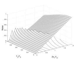
Figure 1: The separability border of the amplification and non-symmetric damping Gaussian system at $t\rightarrow\infty$. The weaker amplification range is defined by $\Gamma_{3}^{2}+4\eta_{1}^{2}<\Gamma_{0}^{2}$.

4 The symmetric amplifier

The system may undergo symmetric single mode amplification as well as the inter-mode amplification, that is $\eta_{3}=0,$ $\eta_{0}\neq 0.$ We consider the situation of weak amplification, that is, $C_{2}>B_{1}$ ($\eta_{0}>0,$ $\Gamma_{3}>0$ is assumed). When $t\rightarrow\infty$, we have $M\rightarrow 0,N\rightarrow 0$, the final state is specified by the residue matrices $\alpha$ and $\beta$ (see Appendix). It seems that the separability criterion might be very complicate, however, a direct calculation shows that the condition can be written as a quadrature form of the square of the inter-mode amplification parameter $\eta_{1},$

$$s_{2}\eta_{1}^{4}+s_{1}\eta_{1}^{2}+s_{0}\geq 0,$$ (19)

with $s_{0}=(1-\eta_{0}^{\prime 2})^{2}[\eta_{0}^{\prime 4}+8(1+\Gamma_{3}^{\prime 2})\eta_{0}^{\prime 2}\overline{n}_{0}(\overline{n}_{0}+1)+16(1-\Gamma_{3}^{\prime 2})^{2}\overline{n}_{0}^{2}(\overline{n}_{0}+1)^{2}],$ $s_{2}=[1-\eta_{0}^{\prime 2}-\Gamma_{3}^{\prime 2}(2\overline{n}_{0}+1)^{2}]^{2},$ $s_{1}=-2\eta_{0}^{\prime 6}-8\eta_{0}^{\prime 4}\overline{n}_{0}(\overline{n}_{0}+1)-2\Gamma_{3}^{\prime 2}\eta_{0}^{\prime 4}(8\overline{n}_{0}^{2}+8\overline{n}_{0}+1)$ $-4(1-\Gamma_{3}^{\prime 2})(1-\Gamma_{3}^{\prime 2}(2\overline{n}_{0}+1)^{2})(2\overline{n}_{0}^{2}+2\overline{n}_{0}+1)$ $+2\eta_{0}^{\prime 2}[8\overline{n}_{0}^{2}+8\overline{n}_{0}+3-4\Gamma_{3}^{\prime 4}\overline{n}_{0}(\overline{n}_{0}+1)(2\overline{n}_{0}+1)^{2}$ $+\Gamma_{3}^{\prime 2}(16\overline{n}_{0}^{4}+32\overline{n}_{0}^{3}+24\overline{n}_{0}^{2}+8\overline{n}_{0}-1)].$

The border of the separable state set and entangled state set is shown in Fig.2 with $\eta_{0}=0.5$ , where only the case of weak amplification is shown. Our numerical result shows that the range (in terms of relative asymmetric damping quantity $\Gamma_{3}^{\prime}=\Gamma_{3}/\Gamma_{0}=(\Gamma_{1}-\Gamma_{2})/(\Gamma_{1}+\Gamma_{2})$ and the noise $\overline{n}_{0}$) of weak amplification shrinks as $\eta_{0}$ increasing, the weak amplification entanglement can only be possible when the noise is less than $1/2$ photon number.

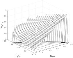
Figure 2: The separability border of the symmetric single-mode amplification, inter-mode amplification and non-symmetric damping Gaussian system at $t\rightarrow\infty$. The weaker amplification case.

5 Conclusion

We have studied the evolution of two-mode Gaussian state under non-symmetric damping, symmetric amplification and thermal noise. The non-symmetric damping is the most general damping of two-mode system. The amplification is limited the symmetric case for simplicity, although the most general case of $\eta_{0}\neq 0,\eta_{1}\neq 0,$ $\eta_{3}\neq 0$ is also solvable. The case of inter-mode amplification alone is especially simple, its separability criterions of final states in both weak and strong amplifications were obtained. The separability criterion of the final state of symmetric amplification ($\eta_{0}\neq 0,\eta_{1}\neq 0,$ $\eta_{3}=0$) is given for weak amplification. Inter-mode amplification parameter $\eta_{1}$ is crucial for entanglement.

In the weak amplification case, final state entanglement is only possible when the thermal noise $\overline{n}_{0}$ is less than $1/2$ photon number. When the single mode amplification parameter $\eta_{0}$ increases, the entanglement range in terms of relative asymmetric damping quantity $\Gamma_{3}^{\prime}=\Gamma_{3}/\Gamma_{0}=(\Gamma_{1}-\Gamma_{2})/(\Gamma_{1}+\Gamma_{2})$, the noise $\overline{n}_{0}$ and inter-mode amplification normalized parameter $\eta_{1}^{\prime}$ shrinks. Lower $\Gamma_{3}^{\prime},$ $\overline{n}_{0}$ and higher $\eta_{1}^{\prime}$ are required for the state to be entangled when $\eta_{0}$ increases.

Appendix: The residue matrices $\alpha$ and $\beta$

In the two mode situation, denote $\alpha=\sum_{i=0}^{3}\alpha_{i}\sigma_{i},$ all $\alpha_{i}$ are real due to $\alpha^{\dagger}=\alpha;$ denote $\beta=\sum_{i=0,1,3}\beta_{i}\sigma_{i},\beta_{i}=\beta_{iR}+i\beta_{iI},$ the $\sigma_{2}$ item is nullified due to $\beta^{T}=\beta.$ Let $\Gamma_{0,3}=\frac{1}{2}(\Gamma_{1}\pm\Gamma_{2}),$ then $\Gamma=\Gamma_{0}\sigma_{0}+\Gamma_{3}\sigma_{3}.$ Together with $\eta=\sum_{i=0,1,3}\eta_{i}\sigma_{i}$ and $\overline{n}=\overline{n}_{0}\sigma_{0}$, all the matrices in Eqs.(3) (4) are expressed in the basis of Pauli matrices. By comparing the coefficient of the Pauli matrices, from Eqs.(3) (4), we obtain two groups of equations, the first group equations containing $\mathbf{\alpha=}(\alpha_{0},\alpha_{1},\alpha_{3})^{T},$ $\mathbf{\beta}_{R}=(\beta_{0R},\beta_{1R},\beta_{3R})^{T}$ are

$$G\mathbf{\alpha-}E\mathbf{\beta}_{R} = (\overline{n}_{0}+\frac{1}{2})(\Gamma_{0},0,\Gamma_{3})^{T}$$

$$E\mathbf{\alpha-}G\mathbf{\beta}_{R} = \mathbf{0}$$

with

$$G=\left[\begin{array}[]{lll}\Gamma_{0}&0&\Gamma_{3}\\ 0&\Gamma_{0}&0\\ \Gamma_{3}&0&\Gamma_{0}\end{array}\right],\text{ }E=2\left[\begin{array}[]{lll}\eta_{0}&\eta_{1}&\eta_{3}\\ \eta_{1}&\eta_{0}&0\\ \eta_{3}&0&\eta_{0}\end{array}\right].$$

The second group equations containing $(\alpha_{2},\beta_{0I},\beta_{1I},\beta_{3I})$ have a solution $(\alpha_{2},\beta_{0I},\beta_{1I},\beta_{3I})=$ $\mathbf{0.}$ The solution to Eqs.(3) (4) is

$$\mathbf{\alpha} = (\overline{n}_{0}+\frac{1}{2})(G-EG^{-1}E)^{-1}(\Gamma_{0},0,\Gamma_{3})^{T}$$

$$\mathbf{\beta} = G^{-1}E\mathbf{\alpha}$$

When $\eta_{3}=0,$ the solution is

$$\alpha = (\overline{n}_{0}+\frac{1}{2})\Delta^{-1}\{(\Gamma_{0}^{2}-4\eta_{0}^{2})[(\Gamma_{0}^{2}-\Gamma_{3}^{2})^{2}+4\Gamma_{3}^{2}(\eta_{1}^{2}-\eta_{0}^{2})-4\Gamma_{0}^{2}(\eta_{1}^{2}+\eta_{0}^{2})]\sigma_{0}$$

$$+4\eta_{0}\eta_{1}[(2\Gamma_{0}^{2}-\Gamma_{3}^{2})(\Gamma_{0}^{2}-\Gamma_{3}^{2})+4\Gamma_{3}^{2}(\eta_{1}^{2}-\eta_{0}^{2})-8\Gamma_{0}^{2}\eta_{0}^{2}]\sigma_{1}$$

$$+\Gamma_{0}\Gamma_{3}[16(2\eta_{0}^{2}-\eta_{1}^{2})(\eta_{0}^{2}-\eta_{1}^{2})+4\eta_{1}^{2}(\Gamma_{3}^{2}-\Gamma_{0}^{2})-8\Gamma_{0}^{2}\eta_{0}^{2}]\sigma_{3}\},$$

$$\beta = (\overline{n}_{0}+\frac{1}{2})\Delta^{-1}\{2\Gamma_{0}\eta_{0}(\Gamma_{0}^{2}-4\eta_{0}^{2})[\Gamma_{0}^{2}-\Gamma_{3}^{2}+4(\eta_{1}^{2}-\eta_{0}^{2})]\sigma_{0}$$

$$+2\Gamma_{0}\eta_{1}[(\Gamma_{0}^{2}-\Gamma_{3}^{2})^{2}+8\eta_{0}^{2}(2\eta_{1}^{2}-2\eta_{0}^{2}-\Gamma_{3}^{2})+4\eta_{1}^{2}(\Gamma_{3}^{2}-\Gamma_{0}^{2})]\sigma_{1}$$

$$+2\eta_{0}\Gamma_{3}[16(\eta_{0}^{2}-\eta_{1}^{2})^{2}+\Gamma_{0}^{2}(\Gamma_{3}^{2}-\Gamma_{0}^{2}-8\eta_{1}^{2})+4\Gamma_{3}^{2}(\eta_{1}^{2}-\eta_{0}^{2})]\sigma_{3}\},$$

where $\Delta=(\Gamma_{0}^{2}-4\eta_{0}^{2})[(\Gamma_{0}^{2}-\Gamma_{3}^{2}-4\eta_{0}^{2}-4\eta_{1}^{2})^{2}-4\eta_{0}^{2}(\Gamma_{3}^{2}+4\eta_{1}^{2})]=(\Gamma_{0}^{2}-4\eta_{0}^{2})[(\Gamma_{0}+2\eta_{0})^{2}-(\Gamma_{3}^{2}+4\eta_{1}^{2})][(\Gamma_{0}-2\eta_{0})^{2}-(\Gamma_{3}^{2}+4\eta_{1}^{2})].$ When $\eta_{0}=\eta_{3}=0,$ the solution is

$$\alpha = \frac{(\overline{n}_{0}+\frac{1}{2})}{\Gamma_{0}\left(\Gamma_{0}^{2}-\Gamma_{3}^{2}-4\eta_{1}^{2}\right)}[\Gamma_{0}(\Gamma_{0}^{2}-\Gamma_{3}^{2})\sigma_{0}+4\Gamma_{3}\eta_{1}^{2}\sigma_{3}],$$

$$\beta = \frac{2(\overline{n}_{0}+\frac{1}{2})\eta_{1}(\Gamma_{0}^{2}-\Gamma_{3}^{2})}{\Gamma_{0}\left(\Gamma_{0}^{2}-\Gamma_{3}^{2}-4\eta_{1}^{2}\right)}\sigma_{1}.$$

References

• [1] D. Walls and G. Milburn, Quantum optics (Springer Verlag, Berlin, 1994).
• [2] D. Petz, An Invitation to the Algebra of Canonical Commutation Relations, Leuven University Press, Leuven (1990).
• [3] A. Perelomov, Generalized Coherent states, Springer Verlag, Berlin (1986).
• [4] X. Y. Chen, Phys. Rev. A, 73, 022307 (2006).
• [5] X. Y. Chen, J. Phys. B, 39, accepted, (2006).
• [6] J. F. Corney, P. D. Drummond, Eprint, quant-ph/0308064, (2003).
• [7] R. Simon, Phys. Rev. Lett. 84, 2726, (2000).
• [8] L. M. Duan , Giedke G, Cirac J I and Zoller P, Phys. Rev. Lett. 84, 2722 (2000).
• [9] L. Z. Jiang, Inter. J. of Quantum Inform. 2, 273 (2004).
• [10] X. Y. Chen, Phys. Rev. A, 71, 062320 (2005).