Which Quantum Evolutions Can Be Reversed by Local Unitary Operations?
Algebraic Classification and Gradient-Flow-Based Numerical Checks

Zusammenfassung

Generalising in the sense of Hahn’s spin echo, we completely characterise those unitary propagators of effective multi-qubit interactions that can be inverted solely by local unitary operations on $n$ qubits (spins-$\tfrac{1}{2}$). The subset of $U\in\mathbf{SU}(2^{n})$ satisfying $U^{-1}=K_{1}UK_{2}$ with pairs of local unitaries $K_{1},K_{2}\in\mathbf{SU}(2)^{\otimes n}$ comprises two classes: in type-I, $K_{1}$ and $K_{2}$ are inverse to one another, while in type-II they are not. Type-I consists of one-parameter groups that can jointly be inverted for all times $t\in\mathbb{R}^{\,}{}$ because their Hamiltonian generators satisfy $KHK^{-1}=\operatorname{Ad_{K}}(H)=-H$. As all the Hamiltonians generating locally invertible unitaries of type-I are spanned by the eigenspace associated to the eigenvalue $-1$ of the local conjugation map $\operatorname{Ad_{K}}$, this eigenspace can be given in closed algebraic form. The relation to the root space decomposition of $\mathfrak{sl}(N,\mathbb{C}^{\,}{})$ is pointed out. Special cases of type-I invertible Hamiltonians are of $p$-quantum order and are analysed by the transformation properties of spherical tensors of order $p$. Effective multi-qubit interaction Hamiltonians are characterised via the graphs of their coupling topology. Type-II consists of pointwise locally invertible propagators, part of which can be classified according to the symmetries of their matrix representations. Moreover, we show gradient flows for numerically solving the decision problem whether a propagator is type-I or type-II invertible or not by driving the least-squares distance $\|K_{1}e^{-itH}K_{2}-e^{+itH}\|{}^{2}_{2}$ to zero.

Introduction

Richard Feynman’s seminal conjecture that quantum systems may be used to efficiently compute and predict the behaviour of other quantum systems Feynman (1982) has inaugurated branches of research inter alia dedicated to Hamiltonian Simulation Lloyd (1996); Abrams and Lloyd (1997); Zalka (1998); Bennett et al. (2002); Masanes et al. (2002); Jané et al. (2003). Actually, backed by the considerations by Manin Manin (2000), Bennett Bennett (1982) and others, it initiated efforts to explore the power of quantum computing. Soon thereafter, sets of universal one- and two-qubit gates were found Deutsch (1985) which allow for decomposing any unitary representation of a quantum computational gate into elementary universal ones.

Exploring computational complexity as well as devising timeoptimal realisations of given quantum algorithms by admissible controls has therefore become an issue of considerable practical interest, see e.g. Khaneja et al. (2001); Schulte-Herbrüggen et al. (2005). In particular the number of computational steps required to implement a quantum gate or to simulate its Hamiltonian is a measure of the actual cost to put the gate or the simulation into practice. A specific question is, whether the sign-inverted Hamiltonian $-H$ can be simulated with only $+H$ and a set of given control Hamiltonians being at hand. The work of Beth et al. has addressed this problem for pair interactions to give bounds on the time-overhead Wocjan et al. (2002a, b); Janzing et al. (2002) required for doing so. In view of effective multi-qubit interactions, here we go beyond pair interactions and classify those Hamiltonians that allow for simulating $-H$ by $H$ and local controls with exact time-overhead $1$.

This is of practical relevance, because when simulating quantum systems one often faces two-part generic tasks: (i) let certain interactions evolve while (ii) other effective multi-qubit interactions shall be suppressed. The latter may be achieved by decoupling, but often it suffices that unwanted interactions cancel at a certain time, e.g. right at the end of an experiment, which is to say they are to be refocussed by inverting them at suitable points in time. This is important for instance to avoid undesired or dissipative coupling of a quantum system to its environment or bath Viola et al. (2000). Many techniques have been developed in magnetic resonance Ernst et al. (1987); Shaka (1996) on the basis of average-Hamiltonian theory Waugh (1996). Moreover, local inversions arise in the context of LOCC, i.e. local operations and classical communication Vidal and Cirac (2002).

Let the operator $T(t)$ denote time translation by $t$ while $\Theta$ represents time reversal. Following Wigner Wigner (1932, 1959) in these very general terms, one immediately finds

$$T(t)\,\circ\,\Theta\,\circ\,T(t)\,\circ\,\Theta={\rm 1\negthickspace l}{}\Leftrightarrow\Theta\,\circ\,T(t)\,\circ\,\Theta=T^{-1}(t)\equiv T(-t)\,.$$ (1)

Now imagine time translation is accompanied by the Hamiltonian unitary evolution of some quantum interaction $H$ according to $U(t)=e^{-itH}$ for all $t$. Then Eqn. 1 turns into

$$\Theta\,\circ\,U(t)\,\circ\,\Theta\;=\;U(-t)\quad.$$ (2)

Clearly time reversal itself is an unphysical operation, however, there are manipulations that bring about effective time reversal for evolutions of certain quantum interactions, the most prominent early example of which being Hahn’s spin echo Hahn (1950).

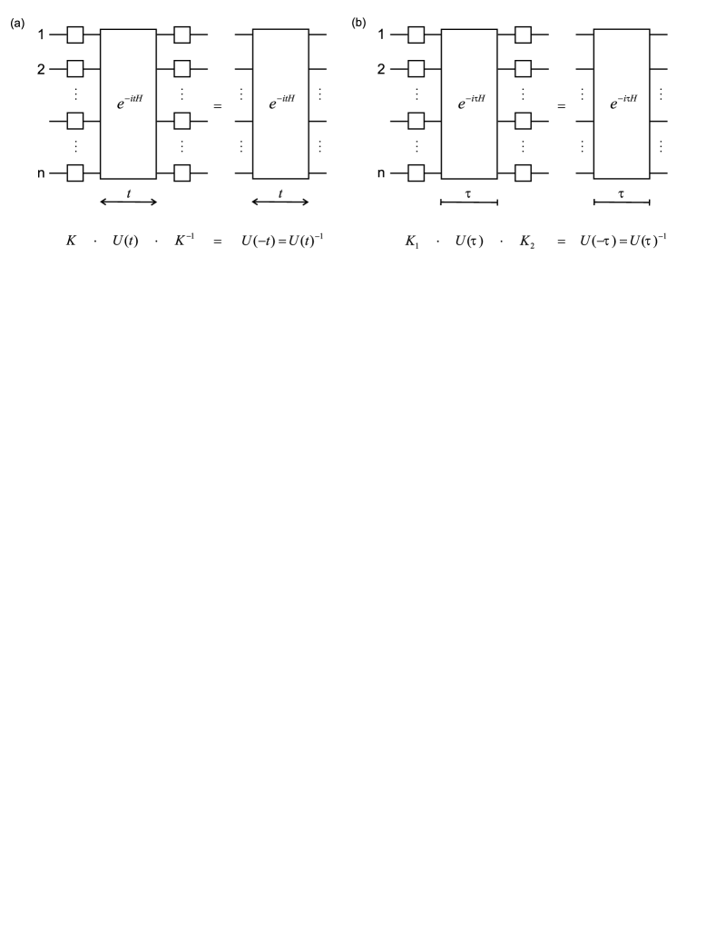
Abbildung 1: There are two non-trivial instances of locally invertible quantum evolutions: (a) in Type-I the interaction can be refocussed by local unitary conjugation with $K\in\mathbf{SU}(2^{n})$ for all times $t\in\mathbb{R}^{\,}{}$. (b) Type-II locally invertible interactions can only be refocussed at specific times $\tau\in\mathbb{R}^{\,}{}$ since $K_{1}$ and $K_{2}$ are not inverse to one another.

Generalising the sense of Hahn’s spin echo, here we ask for which (non-trivial) Hamiltonian evolutions effective time reversal can be obtained by local unitary operations, in other words which Hamiltonian evolutions can be entirely refocussed by framing them solely with local unitaries. As illustrated in Fig. 1 for $n$ qubits, by this we mean: a unitary quantum propagator or gate $U:=e^{-itH}\in\mathbf{SU}(2^{n})$ (with non-zero $t\in\mathbb{R}^{\,}{}$) is invertible exclusively by local unitary operations, if

$$\exists K_{1},K_{2}\in\mathbf{SU}(2)^{\otimes n}:K_{1}e^{-itH}K_{2}=e^{+itH}\;.$$ (3)

Whether or not $K_{1}$ and $K_{2}$ are inverse to one another has implications for universality, as will be shown next.

Case Distinction

As illustrated in Fig. 1, locally invertible propagators exist in two types:

Lemma 0

Either $e^{-itH}$ is trivial and self-inverse, or (i) it is type-I invertible in the sense $\exists K\in\mathbf{SU}(2)^{\otimes n}:KHK^{-1}=-H$ so $Ke^{-itH}K^{-1}=e^{+itH}$ jointly for all $t\in\mathbb{R}^{\,}{}$, or (ii) it is type-II invertible such that at some (but not all) points $\tau$ in time $K_{1}e^{-i\tau H}K_{2}=e^{+i\tau H}$ with $K_{1},K_{2}\in\mathbf{SU}(2)^{\otimes n}$ and $K_{2}^{\phantom{1}}\neq K_{1}^{-1}$.

Tabelle 1: Types of locally invertible interaction evolutions

local invertibility		$K_{2}^{\phantom{1}}=K_{1}^{-1}$		$K_{2}^{\phantom{1}}\neq K_{1}^{-1}$
jointly for all $t\in\mathbb{R}^{\,}{}$		Type-I		$\{\}$
pointwise for some $\tau\in\mathbb{R}^{\,}{}$		self-inverse		Type-II

Since self-inverse cases with $U^{2}={\rm 1\negthickspace l}{}$ (as in the quantum computational cnot, swap and Toffoli gates) are trivial from the point of view of inversion they will be not discussed any further. In order not to bother the reader with a stumbling block, the case distinction of Lemma 0 will be proven in Appendix A.

Organisation and Notation

Rather, for the sake of illustration, we first address the problem of type-I invertibility from a geometric point of view leading to Lie-algebraic terms. A superoperator representation of the adjoint mapping then turns out to reduce the problem to a simple eigenoperator calculation that can be solved algebraically in closed form. This paves the way to discuss pair interaction Hamiltonians. Connecting several pairs then leads to assess local invertibilty in terms of coupling graphs in the case of multi-qubit systems. The transformation properties of multi-qubit interactions seen as spherical tensors of different quantum orders $p$ allow for treating the problem in its normal form, namely invertibility by joint or individual local $z$-rotations. Moreover, the quantum order $p$ relates to the roots of the standard root-space decomposition, which gives necessary and sufficient conditions for local invertibility. After relating the findings to Cartan-like decompositons induced by the concurrence Cartan involution linked to time-reversal symmetry, we finally establish the relation to global minima of the least-squares distance over the restricted group of local unitaries. So invoking the norm property associated with the Frobenius distance, $e^{-itH}$ is locally invertible if and only if

$$\underset{K_{1},K_{2}\in SU(2)^{\otimes n}}{\min}\|K_{1}e^{-itH}K_{2}-e^{+itH}\|{}^{2}_{2}=0\quad,$$ (4)

which can readily be decided on numerically by a gradient flow restricited to the local unitary group.

Type-II invertibility is first treated by establishing symmetry properties for the matrix representations of the interaction Hamiltonians. Then a system of two coupled gradient flows is devised to solve the problem numerically. It can be seen as a flow for the singular-value decomposition (SVD), yet restricted to local unitaries $U$ and $V$.

Throughout the paper, we use the following notation: ${\mathbf{G}}:=\mathbf{SU}(2^{n})$, ${\mathbf{K}}:=\mathbf{SU}(2)\otimes\mathbf{SU}(2)\otimes\cdots\otimes\mathbf{SU}(2)=:\mathbf{SU}(2)^{\otimes n}$ for the Lie groups of the special unitaries and local unitaries as well as ${\mathfrak{g}}$ and ${\mathfrak{k}}$ for their respective Lie algebras. Elements of ${\mathbf{G}}$, ${\mathbf{K}}$, ${\mathfrak{g}}$ and ${\mathfrak{k}}$ are written as $G,K;g,k$ with the only obvious exception of expressing Hamiltonians by $iH\in\mathfrak{g}$.

I Locally Invertible One-Parameter Unitary Groups

Prelude: Geometry

In the single-qubit case, a spin-$\tfrac{1}{2}$ rotation $U({\bf n},\phi)$ by some angle $\phi$ about the axis ${\bf n}$ is—most intuitively—inverted by a $\pi$-rotation about some axis ${\bf n^{\bot}}$ orthogonal to ${\bf n}$ according to

$$U({\bf n},\phi)^{-1}=U({\bf n^{\bot}},\pi)\;U({\bf n},\phi)\;U({\bf n^{\bot}},\pi)^{-1}\quad.$$ (5)

Let the Lie algebra $\mathfrak{su}(2^{n})$ be spanned by some orthonormal basis set $\{a_{j}\}$. Then the generalisation of rotations to higher dimensions, e.g. $n$ qubits (spins-$\tfrac{1}{2}$) is straightforward: replace the rotation axis by the subspace of the Lie algebra $\mathfrak{su}(2^{n})$ that is invariant under the action of $H$

$$I_{H}:={\rm span}_{\mathbb{R}}^{\,}{}\{a_{j}\in\mathfrak{su}(2^{n})\big{|}\;[a_{j},H\,]=0\;\}\quad,$$ (6)

and consider its orthocomplement in $\mathfrak{su}(2^{n})$

$$I^{\bot}_{H}:={\rm span}_{\mathbb{R}}^{\,}{}\{a_{j}\in\mathfrak{su}(2^{n})\big{|}\;a_{j}\not\in I_{H}\;\}\quad.$$ (7)

Making use of the Hilbert space structure Achiezer and Glasman (1981), every $H$ induces a specific decomposition 

$$\mathfrak{su}(2^{n})=I_{H}^{\phantom{\bot}}\,\oplus\,I^{\bot}_{H}\quad.$$ (8)

This setting already implies a particularly simple and illustrative first characterisation of locally invertible unitaries, which, however, is not yet complete:

Lemma 1

For a propagator $U:=e^{-itH}$ to be locally invertible for all $t$, the orthocomplement $I^{\bot}_{H}$ to its invariant subspace in $\mathfrak{su}(2^{n})$ necessarily has to comprise at least one local effective Hamiltonian $k$ with $K:=e^{-ik}\in{\bf SU}(2)^{\otimes n}$.

Proof: Assume there were no local Hamiltonian $k\in I^{\bot}_{\rm H}$: then all the local unitaries $\mathbf{K}={\bf SU}(2)^{\otimes n}$ would be an invariant subgroup to ${\bf SU}(2^{n})$ under the action of the one-parameter unitary group $\{U=e^{-itH}\;|\;t\in\mathbb{R}^{\,}{}\,\}$. In turn, there would be no local unitary to invert a propagator $U=e^{-itH}$ for all $t$. $\blacksquare$

Lemma 2

For a $U=e^{-itH}$ to be locally invertible at all $t$, it is sufficient that there is a local Hamiltonian $k$ in the orthocomplement $I^{\bot}_{\rm H}$ so that the double commutator of $H$ with $k$ reproduces $H$, i.e. $[k,[k,H]]=H$.

Proof: In the first place, note that ${\rm span}_{\mathbb{R}}^{\,}{}\{H,k,i[H,k]\;\}\overset{\rm iso}{=}{}\mathfrak{su}(2)$ implies $[k,[k,H]]=H$, whereas the converse does not necessarily hold. However, the condition $[k,[k,H]]=H$ suffices to define an analytic function

$$f(\phi):=e^{-i\phi k}He^{i\phi k}$$ (9)

with the derivatives

$$\frac{df}{d\phi} = -\;e^{-i\phi k}i[k,H]e^{i\phi k}$$ (10)

$$\frac{d^{2}f}{d\phi^{2}} = -\;e^{-i\phi k}[k,[k,H]]e^{i\phi k}=-f(\phi)\quad.$$ (11)

The boundary conditions $f(0)=H$ and $\tfrac{df}{d\phi}\big{|}_{\phi=0}=-i[k,H]$ allow for expressing the function $f(\phi)$ as

$$e^{-i\phi k}He^{i\phi k}=H\cos\phi-i[k,H]\sin\phi\quad.$$ (12)

For $\phi=\pi$ and $K=e^{-i\pi k}\in\mathbf{SU}(2)^{\otimes n}$ one finds $H\mapsto-H$ so $e^{-itH}$ is locally inverted. $\blacksquare$

However, for obtaining a both necessary and sufficient condition, it seems one has to sacrifice the illustrative simplicity of geometry.

Lemma 3

For a $U=e^{-itH}$ to be locally invertible at all $t$, it is both necessary and sufficient that there is a local Hamiltonian $k$ in the orthocomplement $I^{\bot}_{\rm H}$ and a suitable $\phi\in[0,2\pi[$ with

$$\sum\limits_{\ell=0}^{\infty}\frac{1}{\ell\;!}{\rm ad}^{\ell}_{\,(-i\phi\negthinspace k)}(H)=-H\quad.$$ (13)

Proof: Immediate consequence of the well-known identity

$$e^{X}Ye^{-X}=\sum\limits_{\ell=0}^{\infty}\frac{1}{\ell\,!}{\rm ad}^{\,\ell}_{X}(Y)\quad,$$ (14)

where ${\rm ad}^{\,\ell}_{X}(Y)$ is the $\ell$-fold commutator of $X$ with $Y$, i.e. $[X,[X,\dots[X,Y]\cdots]]$ and $\tfrac{1}{0!}{\rm ad}_{X}^{\,0}:={\rm 1\negthickspace l}{}$. Note this includes Lemma 2 as a special case. $\blacksquare$

Algebra I: Eigenoperators

To begin with, recall the well-known fact that for two matrices $A,B$ to be similar i.e. $XAX^{-1}=B$ with a non-singular $X$, their eigenvalues have to coincide. Thus a Hamiltonian $H$ is invertible by unitary conjugation, if and only if its non-zero eigenvalues (including multiplicity) all occur in pairs of positive and negative sign. This is a necessary and sufficient condition for inversion under some $U\in\mathbf{SU}(2^{n})$, whereas for local unitary inversion by a $K\in\mathbf{SU}(2)^{\otimes n}$ being a special case it is merely a necessary one.

Complete Basis for Locally Invertible Hamiltonians
Although the decomposition of the algebra $\mathfrak{su}(2)^{\oplus n}$ into invariant subspace and orthocomplement is illustrative, it is very tedious to be carried out case-by-case for each and every given Hamiltonian $H$. Rather, in order to obtain constructive parameters, we will turn to the group $\mathbf{SU}(2)^{\otimes n}$ of local unitaries and give a basis set to its eigenspace in which all locally invertible Hamiltonians (of type-I) can be spanned. To this end, observe that due to the series expansion,

$$Ke^{-itH}K^{-1} = e^{-it(KHK^{-1})}=e^{+itH}\quad\forall t\in\mathbb{R}^{\,}{}$$ (15)

$$\Leftrightarrow KHK^{-1} = \operatorname{Ad_{K}}(H)=-H\quad,$$ (16)

where the latter in turn is equivalent to the series expansion of $\operatorname{Ad_{X}}$ in Lemma 3 and Eqn 13. Moreover, by the Kronecker product and the notation of a matrix as a vector (‘vec’) consisting of the matrix columns stacked one upon another Horn and Johnson (1987, 1991) one has illustrated the following obvious necessary and sufficient criterion for local invertibility given as assertion (1)in the following

Lemma 4

(1) The propagator $e^{-itH}$ is locally invertible for all $t\in\mathbb{R}^{\,}{}$ if and only if ${\rm vec}\,H$ is eigenvector of $\operatorname{Ad_{K}}$ (here represented as $K^{*}\,\otimes K$) to the eigenvalue $-1$:

$$(K^{*}\otimes K)\;{\rm vec}\,H=-{\rm vec}\,H\quad.$$ (17)

(2) The eigenspace to the eigenvalue $-1$ spans all the locally invertible Hamiltonians, and it can be given in closed algebraic form by recursively making use of the eigenvectors in $\mathbf{SU}(2)$, as $K\in\mathbf{SU}(2)^{\otimes n}$.

Proof: for assertion (2), we give a constructive proof in view of explicit applications.

Eigenvectors of the $\operatorname{Ad_{K}}$-Superoperator $K^{*}\,\otimes K$:
For any local unitary $K\in\mathbf{SU}(2)^{\otimes n}$, the superoperator $K^{*}\,\otimes K$ is just a $2n$-fold tensor product of unitary $2\times 2$ matrices. Using the quaternion parameterisation

$$U:=\cos\tfrac{\beta}{2}{\rm 1\negthickspace l}{}-i\sin\tfrac{\beta}{2}(n_{x}\sigma_{x}+n_{y}\sigma_{y}+n_{z}\sigma_{z})\in\mathbf{SU}(2)$$ (18)

with $\sum_{\nu=x,y,z}n_{\nu}^{2}=1$, the eigenvalues $\lambda_{\pm}=e^{\pm i\tfrac{\beta}{2}}$ (let $\beta\neq 0$) are associated with the orthonormal eigenvectors

$$v_{+} := \frac{1}{\sqrt{2(1+n_{z})}}\begin{pmatrix}-n_{x}+in_{y}\\ 1+n_{z}\end{pmatrix}$$ (19)

$$v_{-} := \frac{1}{\sqrt{2(1+n_{z})}}\begin{pmatrix}1+n_{z}\\ n_{x}+in_{y}\end{pmatrix}\quad,$$ (20)

where the limit $n_{z}\to-1$ is uncritical: one finds $v_{+}=\left(\begin{smallmatrix}1\\ 0\end{smallmatrix}\right)$ and $v_{-}=\left(\begin{smallmatrix}0\\ 1\end{smallmatrix}\right)$.

One Spin-$\tfrac{1}{2}$ Qubit

The $\operatorname{Ad_{K}}$-superoperator $(K^{*}\,\otimes K)$ for a single spin qubit thus shows the four eigenvalues $\lambda^{*}_{\pm}\lambda^{\phantom{*}}_{\pm}=e^{\mp i\frac{\beta}{2}}e^{\pm i\frac{\beta}{2}}$ (being either 1 or $e^{\pm i\beta}$) associated with the four orthogonal eigenvectors $v^{*}_{\pm}\otimes v^{\phantom{*}}_{\pm}$. Consequently the eigenspace to the overall eigenvalue $e^{\pm i\beta}=-1$ is spanned by the basis set

$$E^{(-)}:=\{v^{*}_{-}\otimes v^{\phantom{*}}_{+},v^{*}_{+}\otimes v^{\phantom{*}}_{-}\}$$ (21)

while the eigenbasis to the overall eigenvalue $+1$ reads

$$E^{(+)}:=\{v^{*}_{+}\otimes v^{\phantom{*}}_{+},v^{*}_{-}\otimes v^{\phantom{*}}_{-}\}\quad.$$ (22)

Remark 1

For fixed parameters $(n_{x},n_{y},n_{z})$ one finds $E^{(-)}\;\bot\;E^{(+)}$. Note, however, that every element in $\mathfrak{su}(2)$ can be spanned in both $E^{(-)}$ and $E^{(+)}$: e.g., vec($\sigma_{z}$) may be expanded in $E^{(-)}$ by $(n_{x},n_{y},n_{z})=(\cos\theta,\sin\theta,0)$, while in $E^{(+)}$ the expansion requires $(n_{x},n_{y},n_{z})=(0,0,1)$. This re-expresses the trivial fact that $\sigma_{z}$ is inverted by any $\pi$ rotation about some axis in the $xy$-plane, whereas it is invariant under $z$ rotation.

For completeness, in the limit $\beta\to 0$ define $E^{(0)}:=\frac{1}{\sqrt{2}}\big{\{}{\rm vec}\,\sigma_{x},{\rm vec}\,\sigma_{y},{\rm vec}\,\sigma_{z}\big{\}}$.

Two Spin-$\tfrac{1}{2}$ Qubits
For two qubits, the eigenbasis to the overall eigenvalue $\lambda^{*}_{1\pm}\lambda^{*}_{2\pm}\lambda^{\phantom{*}}_{1\pm}\lambda^{\phantom{*}}_{2\pm}=-1$ consists of vectors of the following subtypes:

Subtype 0 Embedding of the two limiting $1$-spin cases with $|\beta_{1}|=\pi$ or $|\beta_{2}|=\pi$
$E_{\pi,{\rm 1\negthickspace l}{}}:=\big{\{}E_{1}^{(-)}\otimes{\rm vec}({\rm 1\negthickspace l}{})_{2}^{\phantom{-}}\big{\}}\cup\big{\{}{\rm vec}({\rm 1\negthickspace l}{})_{1}^{\phantom{-}}\otimes E_{2}^{(-)}\big{\}}$

Subtype 1 Inversion of one spin or the other spin with $|\beta_{1}|=\pi,\beta_{2}=0$ or $\beta_{1}=0,|\beta_{2}|=\pi$
$E_{\pi,0}:=\big{\{}E_{1}^{(-)}\otimes E_{2}^{(0)}\big{\}}\cup\big{\{}E_{1}^{(0)}\otimes E_{2}^{(-)}\big{\}}$

Subtype 2 Rotation on both spins with $|\beta_{1}|+|\beta_{2}|=\pi(\operatorname{mod}{\;}2\pi)$ and $\beta_{1},\beta_{2}\neq 0$
$E_{\beta_{1},\beta_{2}}:=\big{\{}E_{1}^{(-)}\otimes E_{2}^{(-)}\big{\}}$

Subtype 3 Rotation on one spin, commutation with the other spin where $|\beta_{1}|=\pi,\beta_{2}\neq 0$ arbitrary, or $|\beta_{2}|=\pi,\beta_{1}\neq 0$ arbitrary
$E_{\pi,\beta^{\parallel}}:=\big{\{}E_{1}^{(-)}\otimes E_{2}^{(+)}\big{\}}\cup\big{\{}E_{1}^{(+)}\otimes E_{2}^{(-)}\big{\}}$

$n$ Spin-$\tfrac{1}{2}$ Qubits
The generalisation to $n$ qubits with

$$\lambda^{*}_{1\pm}\lambda^{\phantom{*}}_{1\pm}\lambda^{*}_{2\pm}\lambda^{\phantom{*}}_{2\pm}\;\cdots\;\lambda^{*}_{\ell\pm}\lambda^{\phantom{*}}_{\ell\pm}\;\cdots\;\lambda^{*}_{n\pm}\lambda^{\phantom{*}}_{n\pm}=-1$$ (23)

is obvious, because the construction follows the pattern described by the indices to the eigenspaces. One may go from $n-1$ spins to $n$ spins by adding the $n$th index from the set $\{{\rm 1\negthickspace l}{},0,\beta,\beta_{\parallel}\}$ to each of the previous $n-1$-spin cases according to the subtype of embedding. Subtype 0 means expand $E_{n-1}$ to $E_{n-1}\otimes{\rm vec{\rm 1\negthickspace l}{}}$; subtype 1 gives $E_{n-1}\otimes E^{(0)}$; subtype 2 leads to $E_{n-1}\otimes E^{(-)}$; subtype 3 results in $E_{n-1}\otimes E^{(+)}$.

In view of constructive results, the above subtypes have been expressed in terms of sets of consistent rotation parameters $(n_{x},n_{y},n_{z})_{\ell}$ and rotation angles $\beta_{\ell}$ on every spin $\ell$. A locally invertible Hamiltonian has to be expandible in at least one set of these self-consistent parameter sets. $\hfill\blacksquare$

In larger spin qubit systems, these checks may become increasingly tedious. However, physical problems are often confined to special settings: a Hamiltonian may be constituted by pair interactions, or in other instances, a Hamiltonian may be made up of terms that can be grouped in combinations of interactions transforming like spherical tensors of various $p$-quantum order. For these two practically relevant cases, we present more convenient methods.

Ising and Heisenberg Pair Interactions

Tabelle 2: Type-I Invertibility of Elementary Pair Interactions

Pair		Expansion		Type-I Local		Symmetry
Interaction		in Subtype		Inversion by		Class
ZZ		$E_{\pi,0}$		$\pi(\perp 1)$ or: $\pi(1\perp)$		(0,2)(9,0)[0,0]
XX		$E_{\pi,0}$		$\pi(z1)$ or: $\pi(1z)$		(0,2)(9,0)[0,0]
		$E_{\beta_{1},\beta_{2}}$		$\beta_{1}(z1)-\beta_{2}(1z)$		(0,2)(9,0)[0,0]
				[e.g.: $\tfrac{\pi}{2}(z1-1z)$]		(0,2)(9,0)[0,0]
		$E_{\pi,\beta^{\parallel}}$		$\pi(\perp 1)-\pi(1\dashv)$		(0,2)(9,0)[0,0]
XY		$E_{\pi,0}$		$\pi(z1)$ or: $\pi(1z)$		(0,2)(9,0)[0,0]
		$E_{\pi,\beta^{\parallel}}$		$\pi(x1)\pm\pi(1y)$		(0,2)(9,0)[0,0]
				or: $\pi(y1)\pm\pi(1x)$
X(-X)		$E_{\pi,0}$		$\pi(z1)$ or: $\pi(1z)$		(0,2)(9,0)[0,0]
		$E_{\beta_{1},\beta_{2}}$		$\beta_{1}(z1)+\beta_{2}(1z)$		(0,2)(9,0)[0,0]
				[esp.: $\tfrac{\pi}{2}(z1+1z)$]		(0,2)(9,0)[0,0]
		$E_{\pi,\beta^{\parallel}}$		$\pi(\perp 1)+\pi(1\vdash)$		(0,2)(9,0)[0,0]
XXX		none		–		–
XXY		none		–		–
XYZ		none		–		–

The pair interactions of Ising and Heisenberg type can easily be related to the $-1$ eigenspaces as summerised in Tab. 2: while the Ising-$ZZ$ interaction can only be expanded in the eigenspaces of Subtype 1, i.e. $E_{\pi,0}$, Heisenberg-$XX$ and $XY$ interactions allow for expansions in Subtype 1 as well as Subtype 2 ($E_{\beta_{1},\beta_{2}}$).

For brevity, in the table we use the short-hand notation $(z1)$ for $\tfrac{1}{2}(\sigma_{z}\otimes{\rm 1\negthickspace l}{})$, and $(z1\pm 1z$) for $\tfrac{1}{2}(\sigma_{z}\otimes{\rm 1\negthickspace l}{}\pm{\rm 1\negthickspace l}{}\otimes\sigma_{z})$. as well as $(\perp 1)$ for $\tfrac{1}{2}(\sigma_{x}\cos\phi+\sigma_{y}\sin\phi)\otimes{\rm 1\negthickspace l}{}$ and analogously with reference to some fixed $\phi$ we write $(\dashv)$ and $(\vdash)$ for $\tfrac{1}{2}(\sigma_{x}\cos(\phi\pm\tfrac{\pi}{2})+\sigma_{y}\sin(\phi\pm\tfrac{\pi}{2}))$. For example, the Heisenberg $XX$ interaction can of course be inverted by $\pi$ $z$-pulses on one or the other qubit, but also by an antisymmetric $z$-rotation on both qubits, where the rotation angle is $\beta$ on qubit 1 and $\beta-\pi$ on qubit 2. Note that inverting generic $ZZ$, $XX$, and $XY$ interactions requires pulses that are non-symmetric with regard to permuting qubits 1 and 2. In view of convenient extensions to networks of pair interactions, we write  $\multiputlist(0,2)(9,0)[0,0]{{\hskip 7.11317pt\circle*{5.0}},{\line(1,0){15.0}},{\hskip 7.11317pt\circle{5.0}}}$    for a pair interaction of two qubits that is inverted by such non-symmetric local pulses. The only exception of different symmetry is the Heisenberg $X(-X)$ interaction, since it can also be inverted by a permutation symmetric $\tfrac{\pi}{2}$ $z$-pulse on both of the qubits expressed by  $\multiputlist(0,2)(9,0)[0,0]{{\hskip 7.11317pt\circle*{5.0}},{\line(1,0){15.0}},{\hskip 7.11317pt\circle*{5.0}}}$   .

Note that none of the Heisenberg $XXX$ or $XXY$ or $XYZ$ interactions is type-I invertible by local unitaries, because their interaction Hamiltonians already fail the simple necessary condition of being invertible over the entire unitary group: their non-zero eigenvalues do not occur in pairs of opposite sign. For instance, the eigenvalues to the $XYZ$ interaction Hamiltonian $H_{XYZ}:=\alpha(\sigma_{x}\otimes\sigma_{x})+\beta(\sigma_{y}\otimes\sigma_{y})+\gamma(\sigma_{z}\otimes\sigma_{z})$ read

$$\begin{split}\lambda_{1}&=+\alpha+\beta-\gamma\\ \lambda_{2}&=-\alpha+\beta+\gamma\\ \lambda_{3}&=+\alpha-\beta+\gamma\\ \lambda_{4}&=-\alpha-\beta-\gamma\end{split}$$ (24)

with $\alpha,\beta,\gamma\in\mathbb{R}^{\,}{}$. Clearly, unless at least one of the parameters $\{\alpha,\beta,\gamma\}$ vanishes, there are no pairs of opposite sign thus limiting the type-I invertible interactions to $ZZ$ or $XX$ or $XY$ type.

Coupling Graphs for Networks of Pair Interactions

Coupling networks made up by pair interactions between qubits can conveniently be represented by graphs: each vertex denotes a qubit, and an edge connecting two qubits $k$ and $l$ then corresponds to a non vanishing pair interaction or coupling $J_{kl}$. These may take the form of any of Ising or Heisenberg type interactions described before. We will discuss connected graphs that do not necessarily have to be complete.

As will be seen next, interactions with coupling topologies of bipartite graphs have special properties.

Abbildung 2: In a bipartite coupling graph, only vertices of different colour $\circ$ or $\bullet$ are pairwise connected.

Lemma 5 (Variant to Beth Wocjan et al. (2002a))

The evolution under Ising $ZZ$-interactions

$$H_{ZZ}:=\pi\sum\limits_{k<l}^{n}J_{kl}\;\tfrac{1}{2}\sigma_{kz}\otimes\sigma_{lz}$$ (25)

is type-I invertible by local unitary operations if and only if its coupling topology of non-vanishing couplings $J_{kl}$ forms a bipartite graph.

Proof:
(i) For $H_{ZZ}\mapsto-H_{ZZ}$ it is sufficient that each of the edges of the coupling graph is inverted. Using local actions on the vertices, this means every vertex of either the type $\bullet$ (or $\circ$) has to be inverted an odd number of times, while the other type $\circ$ (or $\bullet$) remains invariant i.e. is inverted an even number of times incl. zero.
(ii) Not only is this condition sufficient, it is also necessary: assume there were edges connecting two vertices of the same type (either $\bullet$ or $\circ$). Then the couplings depicted by such edges would not be inverted, as they flip their signs twice (or an even number of times) thus remaining effectively invariant. $\blacksquare$

Lemma 6

The evolution under the Heisenberg $XY$-interaction

$$H_{XY}:=\pi\sum\limits_{k<l}^{n}J_{kl}\;\tfrac{1}{2}\big{(}\sigma_{kx}\otimes\sigma_{lx}+\kappa\;\sigma_{ky}\otimes\sigma_{ly}\big{)}\;,$$ (26)

where $\kappa\in\;[-1;+1]$ is type-I invertible by local unitary operations if and only if (i) either its topology of non-vanishing couplings $J_{kl}$ forms a bipartite graph or (ii) $\kappa=-1$, in which case the coupling topology may take the form of any connected graph.

Proof:
Let $F_{\nu}$ with $\nu\in\{x,y,z\}$ denote the sum over $n$ qubits with the Pauli matrix $\sigma_{\nu}^{(\ell)}$ in the $\ell^{\rm th}$ place

$$F_{\nu}:=\tfrac{1}{2}\sum\limits_{\ell=1}^{n}{\rm 1\negthickspace l}{}^{(1)}\otimes{\rm 1\negthickspace l}{}^{(2)}\otimes\cdots\otimes{\rm 1\negthickspace l}{}^{(\ell-1)}\otimes\sigma_{\nu}^{(\ell)}\otimes{\rm 1\negthickspace l}{}^{(\ell+1)}\otimes\cdots\otimes{\rm 1\negthickspace l}{}^{(n)}$$ (27)

and analogously write $F_{z}^{(\circ)}$ or $F_{z}^{(\bullet)}$ if the sum just extends over all qubits coloured $\circ$ or $\bullet$, respectively.
(i) For $\kappa\in\;]-1;+1]$ a bipartite coupling topology suffices to allow for the inversion $H_{XY}\mapsto-H_{XY}$ by the rotations $\pi F_{z}^{(\circ)}$ or $\pi F_{z}^{(\bullet)}$. A bipartite topology is also necessary, since in general no permutation-symmetric inversion of $H_{\rm XY}$ exists (see Tab. 2).
(ii) Cleary, also in the special case $\kappa=-1$ a bipartite coupling graph suffices. However, it is not necessary, because a $\tfrac{\pi}{2}$ $z$-rotation on all the qubits ($\tfrac{\pi}{2}\;F_{z}$) is invariant under qubit permutation and thus does the same job on any connected coupling graph without requiring the distinction of a bipartite topology (cp the permutation symmetric inversion of the $X(-X)$ interaction in Tab. 2). $\blacksquare$

Examples of Pair Interaction Hamiltonians

For instance, neither Ising ZZ-coupling nor the Heisenberg XX and XY interactions on a cyclic three-qubit coupling topology ($C_{3}$) are type-I invertible, because $C_{3}$ is clearly not bipartite. However, also on $C_{3}$, the Heisenberg X(-X)-interaction is type-I invertible, as will be illustrated below in the section on gradient flows.

Extension to Effective Multi-Qubit Interactions

In multi-qubit effective interaction Hamiltonians on a coupling graph $G$, the interaction order $\ell$ (e.g. $\ell=3$ for $H_{\rm eff}=\sigma_{z}\otimes\sigma_{z}\otimes\sigma_{z}/2$) may be used to group terms of different order. To each order, there is a subgraph $G_{m_{\ell}}$.

Lemma 7

Let $H_{\rm eff}$ be an effective multi-qubit interaction Hamiltonian constituted by the $\ell$-interaction terms on the $m_{\ell}$ subgraphs.

$$H_{\rm eff}=\sum\limits_{\ell,m_{\ell}}H_{\ell,{m_{\ell}}}$$ (28)

where $\ell$ runs over the interaction orders and $m_{\ell}$ comprises all the $\ell$-order interaction terms on subgraphs $G_{m_{\ell}}$.

Then $H_{\rm eff}$ is locally invertible of type-I if and only if its constituents on the $G_{m_{\ell}}$ are all simultaneous eigenoperators of some $\operatorname{Ad}_{K}$ to the eigenvalue $-1$.

Proof:
The interaction order as well as the assignment to the subgraphs is $\operatorname{Ad}_{K}$ invariant. $\blacksquare$

In simpler cases, the grouping may help to find local inversions by paper and pen. However, more complicated multi-qubit interactions can be treated by exploiting the transformation properties in terms of spherical tensors, as will be shown next.

Sequences of Interaction Propagators

Clearly, a palindromic sequence of propagators

$$U_{s}U_{s-1}\cdots U_{2}U_{1}U_{1}U_{2}\cdots U_{s-1}U_{s}$$ (29)

is locally invertible, if either each component $U_{k}$ or at least one partitioning of the sequence is locally invertible.

Multi-Qubit Interaction Hamiltonians of $p$-Quantum Order

As usual in the treatment of angular momenta in spin-$j$ representation (where $j=n\,\cdot\,j^{\prime}$ may sum the spin quantum numbers of $n$ identical, i.e. permutation symmetric single spins-$j^{\prime}$ to the group spin-$j$) one defines a rank-$j$ spherical tensor $T_{j,m}{}$ of order $m$ by the transformation properties under rotation by the Euler angles $\{\alpha,\beta,\gamma\}$

$$\begin{split}D^{(j)}(\alpha,\beta,\gamma)\,\,&T_{j,m}{}\,\,{D^{(j)}(\alpha,\beta,\gamma)}^{-1}\\ &=\sum_{m^{\prime}=-j}^{j}\,D_{m^{\prime},\,m}^{(j)}(\alpha,\beta,\gamma)\,T_{j,m^{\prime}}{}\,,\end{split}$$ (30)

where the elements

$$\begin{split}D_{m^{\prime},\,m}^{(j)}(\alpha,\beta,\gamma):&=\langle j,\,m^{\prime}|e^{-i\frac{\alpha}{2}\,\sigma_{z}^{(j)}}e^{-i\frac{\beta}{2}\,\sigma_{y}^{(j)}}e^{-i\frac{\gamma}{2}\,\sigma_{z}^{(j)}}\,\,j,\,m\rangle{}\\ &=e^{-im^{\prime}\alpha}\,\,\,d_{m^{\prime},\,m}^{(j)}(\beta)\,\,e^{-im\gamma}\end{split}$$ (31)

constitute the full Wigner rotation matrix. An equivalent definition of the spherical tensors via the Pauli matrices or angular momentum operators $\{J_{x},J_{y},J_{z}\}\overset{\rm iso}{=}{}i\;\mathfrak{su}(2)$ in spin-$j$ representation uses the commutation relations

$$\begin{split}[J_{x}\pm iJ_{y},T_{j,m}{}]\,&\equiv[J^{\pm},T_{j,m}{}]\,\\ &=\,\sqrt{j(j+1)-m(m\pm 1)}\,\,\,T_{j,m\pm 1}{}\\ [J_{z},T_{j,m}{}]\,&=\,m\,T_{j,m}{}\end{split}$$ (32)

and establishes the relation to the algebra $\mathfrak{sl}(2,\mathbb{C}^{\,}{})$ represented by $\{J_{+},J_{-},J_{z}\}$, as will be further illustrated below.

Now specialise $D^{(j)}(\alpha,\beta,\gamma)$ to $D^{(j)}(0,0,\phi)$ by setting $\alpha=\beta=0$ and $\gamma\equiv\phi$. Moreover, identify $m=m^{\prime}$ with the quantum order $p$ of the interaction Hamiltonian $H\equiv T_{j,p}{}$ to obtain the eigenoperator equation

$$D^{(j)}(0,0,\phi)\;\;T_{j,p}{}\;\;{D^{(j)}(0,0,\phi)}^{-1}=e^{-ip\phi}\;T_{j,p}{}\,.$$ (33)

Inversion by Joint Local $z$-Rotations

Note that the commutation relations for $\mathfrak{su}(2)$ or $\mathfrak{sl}(2,\mathbb{C}^{\,}{})$ do not change, if one replaces the $J_{\nu}$ where $\nu\in\{x,y,z;+,-\}$ by the symmetric sum over $n$ qubits with $J_{\nu}^{(\ell)}$ in the $\ell^{\rm th}$ place written again as

$$F_{\nu}:=\sum\limits_{\ell=1}^{n}{\rm 1\negthickspace l}{}^{(1)}\otimes{\rm 1\negthickspace l}{}^{(2)}\otimes\cdots\otimes{\rm 1\negthickspace l}{}^{(\ell-1)}\otimes J_{\nu}^{(\ell)}\otimes{\rm 1\negthickspace l}{}^{(\ell+1)}\otimes\cdots\otimes{\rm 1\negthickspace l}{}^{(n)}\,.$$ (34)

Therefore, we may also envisage $D^{(j)}(0,0,\phi)$ as a local $z$-rotation by an angle $\phi$ acting jointly on all the $n$ qubits, i.e., $D^{(j)}(0,0,\phi)=:K(\phi,F_{z})\in\mathbf{SU}(2)^{\otimes n}$. Thus one arrives at the two identical formulations

$$\begin{split}K(\phi,F_{z})\;\;T_{j,p}{}\;\;{K(\phi,F_{z})}^{-1}&=e^{-ip\phi}\;T_{j,p}{}\\ \operatorname{Ad}_{K(\phi,F_{z})}T_{j,p}{}\,\,&=e^{-ip\phi}\;T_{j,p}{}\;.\end{split}$$ (35)

Clearly, inverting $T_{j,p}{}$ to $-T_{j,p}{}$ requires $e^{-ip\phi}=-1$. By the Fourier duality between the quantum order $p$ and the phase $\phi$ one readily finds the results given in Table 3. A joint local $z$-rotation of angle $\pi/r$ (with a fixed $r=1,2,3,\dots$) simultaneously inverts all the rank-$j$ tensors of different quantum orders $p$ given in the same row of the table. Thus also any linear combination of interaction tensors of quantum orders $\pm p=r(2q+1)$ can be inverted at a time for all $q=1,2,3,\;\dots$ .

Tabelle 3: Inversion of Spherical Tensors by Joint $z$-Rotations

rotation angle $\phi$		inverts interactions of quantum order $\pm p$
${\pi}$		$1,3,5,\cdots,2q+1\;\leq\;j$
${\pi}/{2}$		$2,6,10,\cdots,4q+2\;\leq\;j$
${\pi}/{3}$		$3,9,15,\cdots,6q+3\;\leq\;j$
$\vdots$		$\vdots$
${\pi}/{r}$		$r,3r,5r,\cdots,r\,(2q+1)\;\leq\;j$

Obviously, interaction Hamiltonians represented by spherical tensors $T_{j,0}{}$ of order $p=0$ cannot be inverted by $z$-rotations $K(\phi,F_{z})$, but may possibly be inverted by local unitaries operating on other than the $z$-axes. However, rank-$0$ tensors $T_{0,0}{}$ transforming like pseudoscalars such as e.g. the Heisenberg $XXX$ interaction Hamiltonian, which in two spins is proportional to

$$T_{0,0}{}=\frac{-1}{2\sqrt{3}}\;\big{(}\sigma_{x}\otimes\sigma_{x}+\sigma_{y}\otimes\sigma_{y}+\sigma_{z}\otimes\sigma_{z}\big{)}\;,$$ (36)

cannot be inverted at all. Not only does this hold for local unitaries, but for any similarity transform by some $X\in\mathbf{GL}(2^{n})$, since the non-zero eigenvalues of $T_{0,0}{}$ do not occur in pairs of opposite sign (vide supra).

Inversion under Individual Local $z$-Rotations

Since in a single spin qubit, $\operatorname{Ad_{\phi,z}}$ has the eigenoperators $J_{\nu}\in\{{\rm 1\negthickspace l}{},J_{z},J_{+},J_{-}\}$ associated to the respective eigenvalues $e^{-ip_{\nu}\phi}\in\{1,1,e^{-p_{+}\phi},e^{-p_{-}\phi}\}$, it is easy to generalise the previous arguments to the case of $z$-rotations on $n$ qubits—but with individually differing rotation angles on each spin qubit $\phi_{1},\phi_{2},\dots,\phi_{\ell},\dots,\phi_{n}$. Now consider a Hamiltonian $\bar{H}$ taking the special form of a tensor product of $\operatorname{Ad_{\phi,z}}$ eigenoperators on each spin qubit $\ell=1,\dots,n$ according to

$$\bar{H}:=J_{\nu_{1}}^{(1)}{}\otimes J_{\nu_{2}}^{(2)}{}\otimes\cdots\otimes J_{\nu_{\ell}}^{(\ell)}{}\otimes\cdots\otimes J_{\nu_{n}}^{(n)}{}$$ (37)

with independent $\nu_{\ell}\in\{{\rm 1\negthickspace l}{},z,+,-\}$ on each spin qubit. Then $\bar{H}$ is clearly an eigenoperator to individual local $z$-rotations $K(\phi_{1},\;\dots\;,\phi_{n},F_{z})\in\mathbf{SU}(2)^{\otimes n}$ by virtue of

$$\operatorname{Ad_{K(\phi_{1},\;\dots\;,\phi_{n},F_{z})}}\big{(}\bar{H}\big{)}=e^{-i(p_{1}\phi_{1}+\;\cdots\;+p_{n}\phi_{n})}\;\bar{H}\;.$$ (38)

So $\bar{H}$ is inverted if there is a set of rotation angles $\{\phi_{\ell}\}$ with

$$\sum\limits_{\ell=1}^{n}p_{\ell}\phi_{\ell}=\pm\pi\;(\operatorname{mod}{\;}2\pi)\quad,$$ (39)

which is the case if there is at least one spin qubit $\ell$ giving rise to an interaction of quantum order $p_{\ell}=\pm 1$. Moreover, a linear combination of such Hamiltonians $\bar{H}_{\Sigma}:=\sum\limits_{\lambda=1}^{m}c_{\lambda}\bar{H}_{\lambda}$ is jointly invertible by an individual local $z$-rotation $K(\phi_{1},\;\dots\;,\phi_{n},F_{z})$ , if there is at least one consistent set of rotation angles $\{\phi_{\ell}\}$ simultaneously satisfying for all the components $\bar{H}_{\lambda}$

$$\sum\limits_{\ell=1}^{n}p_{\lambda,\ell}\;\cdot\;\phi_{\ell}=\pm\pi\;(\operatorname{mod}{\;}2\pi)\;,$$

which expresses the linear system

$$\begin{pmatrix}p_{11}&p_{12}&\cdots&p_{1n}\\ p_{21}&p_{22}&\cdots&p_{2n}\\ p_{31}&p_{32}&\cdots&p_{3n}\\ \vdots&\vdots&\ddots&\vdots\\ p_{m1}&p_{m2}&\cdots&p_{mn}\\ \end{pmatrix}\begin{pmatrix}\phi_{1}\\ \phi_{2}\\ \vdots\\ \phi_{n}\end{pmatrix}=\begin{pmatrix}\pm\pi\;(\operatorname{mod}{\;}2\pi)\\ \pm\pi\;(\operatorname{mod}{\;}2\pi)\\ \pm\pi\;(\operatorname{mod}{\;}2\pi)\\ \vdots\\ \pm\pi\;(\operatorname{mod}{\;}2\pi)\end{pmatrix}\;.$$ (40)

Note the signs on the rhs may be chosen independently in $2^{m}$ ways with every choice forming a system of $m$ linear equations in $n$ variables. Therefore, if the vector of any of the combinations $\pi\;(\pm 1,\pm 1,\;\cdots\;,\pm 1)^{t}$ can be expanded in terms of the column vectors of $P:=\big{(}p_{\lambda,\ell}\big{)}$ with real coefficients, then $\bar{H}_{\Sigma}$ is locally invertible by $z$-rotations. In the special case of $m=n$ and $P$ non-singular, there always is a consistent set of individual rotation angles for inverting $\bar{H}_{\Sigma}$ for any choice of signs. For simplicity, we will drop the index $\Sigma$ in $\bar{H}_{\Sigma}$ henceforth writing $\bar{H}$ for Hamiltonians locally invertible by individual $z$-rotations.

Corollary 1

Let $\bar{H}$ be locally invertible by individual $z$-rotations on each qubit. Then the following hold.

• Any Hamiltonian $H$ on the local unitary orbit $\operatorname{Ad_{\mathbf{K}}}(\bar{H})$ of any such $\bar{H}$ generates a one-parameter unitary group that is locally invertible of type-I.

• In turn, any type-I locally invertible Hamiltonian $H$ is on a local unitary orbit of some $\bar{H}$.

Proof: (1) is obvious. (2) follows since every local unitary $K$ is locally unitarily similar to a local $z$-rotation $K_{z}$: $K=\bar{K}K_{z}\bar{K}^{-1}\Rightarrow KHK^{-1}=-H\Leftrightarrow K_{z}\bar{H}K_{z}^{-1}=-\bar{H}$ where $\bar{H}:=\bar{K}^{-1}H\bar{K}$. $\blacksquare$
Thus local invertibility by $z$-rotations can be looked upon as the normal form of the problem.

Moreover, in order to see the link to the root space decomposition of the semisimple Lie algebra $\mathfrak{sl}(2,\mathbb{C}^{\,}{})$ in spin-$j$ representation, take the derivative of Eqn. 35

$$\frac{\partial{}}{\partial{\phi}}\,\,{}\big{|}_{\phi=0}\operatorname{Ad}_{K(\phi,z)}T_{j,p}{}\,\, = \frac{\partial{}}{\partial{\phi}}\,\,{}\Big{|}_{\phi=0}e^{-ip\phi}\;T_{j,p}{}$$ (41)

$$\Leftrightarrow\;-i\operatorname{ad}_{k_{z}}(T_{j,p}{}) = -ip\;T_{j,p}{}\;.$$ (42)

(NB: the minus sign on the left side of the last identity is due to the convention $K(\phi,z):=e^{-i\phi k_{z}}$ analogous to $U:=e^{-itH}$ imposed by Schrödinger’s equation.)

Note the tensors are eigenoperators to $\operatorname{ad}_{k_{z}}$ of the joint local $z$-rotations as anticipated in Eqn. 32.

Algebra II: Root-Space Decomposition

To fix notations, let $\mathfrak{g}$ be a complex semisimple Lie algebra and let $\mathfrak{g}_{0}$ be a Cartan subalgebra of $\mathfrak{g}$, i.e. a maximally abelian subalgebra such that for all $H\in\mathfrak{g}_{0}$, the commutator superoperators $\operatorname{ad}_{H}$ are simultaneously diagonalisable. Then the root-space decomposition of $\mathfrak{g}$ with respect to $\mathfrak{g}_{0}$ takes the form

$$\mathfrak{g}=\mathfrak{g}_{0}\oplus\bigoplus_{\alpha\neq 0}\mathfrak{g}_{\alpha}\quad,$$ (43)

where the root-spaces $\mathfrak{g}_{\alpha}$ (with $\alpha\neq 0$) are the non-trivial simultaneous eigenspaces

$$\mathfrak{g}_{\alpha}:=\{g\in\mathfrak{g}\,|\,\operatorname{ad}_{H}(g)=\alpha(H)\,g\,\}\quad.$$ (44)

The corresponding non-trivial $\alpha$’s are called roots of the decomposition. They are elements of the dual space $\mathfrak{g}_{0}^{*}$ of linear functionals on $\mathfrak{g}_{0}$.

In the following, we consider the complex semisimple Lie algebra $\mathfrak{sl}(N,\mathbb{C}^{\,}{})$ as the complexification of the real Lie algebra $\mathfrak{su}(N)$. Define $E_{ij}$ as a square matrix differing from the zero matrix by just one element—the unity in the $j^{\rm th}$ column of the $i^{\rm th}$ row. Moreover, let $\mathfrak{g}_{0}$ be the set of all diagonal matrices in $\mathfrak{sl}(N,\mathbb{C}^{\,}{})$ and define $e_{i}(H):=H_{ii}$ for all $H\in\mathfrak{g}_{0}$. Then for every $H\in\mathfrak{g}_{0}$, the $E_{ij}$ are simultaneous eigenoperators of the commutator superoperators $\operatorname{ad}_{H}$ with eigenvalues depending linearly on $H$

$$\begin{split}\operatorname{ad}_{H}(E_{ij})&=(H_{ii}-H_{jj})\,E_{ij}\\ &=\big{(}e_{i}(H)-e_{j}(H)\big{)}\,E_{ij}=:\alpha_{ij}E_{ij}\quad.\end{split}$$ (45)

Thus the root-space decomposition of $\mathfrak{sl}(N,\mathbb{C}^{\,}{})$ may be rewritten as

$$\mathfrak{g}=\mathfrak{g}_{0}\oplus\;\bigoplus\limits_{i\neq j}\mathbb{C}^{\,}{}E_{ij}\quad.$$ (46)

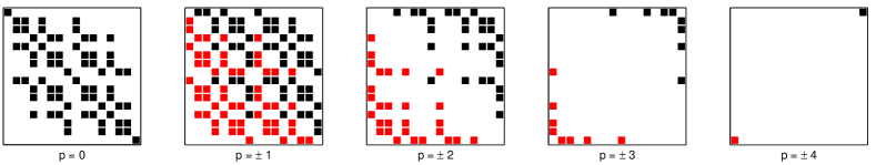
Abbildung 3: (Colour online) Matrices $E_{ij}$ constituting the rank-$4$ spherical tensors $T_{4,p}$ of order $p$ (here in a system of $4$ spins-$\tfrac{1}{2}$, $p\in[-4,+4]$). The non-zero elements in the $E_{ij}$ are marked $\blacksquare$ for $p\geq 0$ and $\blacksquare$ for $p<0$. The $T_{4,p}$ are eigenoperators to the Weyl torus element $F_{z}\in\mathfrak{t}$ according to $\operatorname{ad}_{F_{z}}(T_{4,p})=p\;T_{4,p}$ with the eigenvalues being the quantum orders $p$. The constituents of the tensors are the single-element Weyl matrices $E_{ij}$ sharing the same eigenvalues $\operatorname{ad}{F_{z}}(E_{ij})=p\;E_{ij}$. According to Tab. 3, a Hamiltonian comprising elements that transform like $T_{4,\pm p}$ can locally be sign-inverted e.g. by a joint $z$-rotation of angle $\pi/p$.

Furthermore, if $\mathfrak{g}^{\prime}$ is a compact real semisimple Lie algebra with maximally torus algebra $\mathfrak{t}^{\prime}$, then the complexification $\mathfrak{t}$ of $\mathfrak{t}^{\prime}$ gives a Cartan subalgebra of the complexification $\mathfrak{g}$ of $\mathfrak{g}^{\prime}$. For example in the case of $\mathfrak{su}(N)$,

$$\mathfrak{t}^{\prime}:=\{i\,\operatorname{diag}{}(\theta_{1},\theta_{2},\,\dots\,,\theta_{N})\,|\,\sum_{\ell}\theta_{\ell}=0\}$$ (47)

may be chosen as maximal torus algebra. Then

$$\mathfrak{t}:=\mathfrak{t^{\prime}}+i\,\mathfrak{t^{\prime}}$$ (48)

i.e. the set of all complex diagonal matrices forms the Cartan subalgebra of $\mathfrak{sl}(N,\mathbb{C}^{\,}{})$.

Now Eqn. 45 shows that an $E_{ij}$ with $i\neq j$ can be sign-inverted provided $(H_{ii}-H_{jj})\neq 0$. The generic case, joint and individual local $z$-rotations are specified next.

Proposition 1

In a system of $n$ spins-$\tfrac{1}{2}$, for the single-element matrices $E_{ij}$ with $i\neq j$ the following hold:

• to any $E_{ij}$ there is an element of the Weyl torus taking the form $T=\exp(-i\operatorname{diag}{}\big{(}\theta_{1},\theta_{2},\,\dots\,,\theta_{N})\big{)}$ so that $\operatorname{Ad}_{T}(E_{ij})=-E_{ij}$;

• any matrix $E_{ij}$ can also be sign-inverted by a single local $z$-rotation;

• in contrast, by a joint local $z$-rotation on all the $n$ spins-$\tfrac{1}{2}$, an $E_{ij}$ can only be sign-inverted if for its indices $i,j$ the reductions by $1$ written as binary numbers $(i-1)_{2}$ and $(j-1)_{2}$ do not have the same number of $0$’s and $1$’s (irrespective of the order).

Proof: First, note that although $\mathfrak{sl}(2^{n},\mathbb{C}^{\,}{})$ comprises the generators of all special unitary propagators, its maximally abelian subalgebra $\mathfrak{g}_{0}$ can—without loss of generality—always be chosen such that it includes the generators of all the local $z$-rotations. They suffice to be considered, since the $E_{ij}$ are simultaneous eigenoperators to all elements in $\mathfrak{g}_{0}$.

(1) Obviously elements in the Weyl torus algebra $\mathfrak{t}$ can be chosen such that $\theta_{i}-\theta_{j}\neq 0$.

(2) Clearly any off-diagonal element $E_{ij}$ in the boxes of the block matrix $H:=\begin{pmatrix}\phantom{.}{\rm 1\negthickspace l}{}&\Box\\ \Box&-{\rm 1\negthickspace l}{}\end{pmatrix}$ is associated with a non-zero root $(e_{i}-e_{j})(H)=H_{ii}-H_{jj}$. The same holds true for $H\otimes{\rm 1\negthickspace l}{}$ and ${\rm 1\negthickspace l}{}\otimes H$. Likewise any off-diagonal element $E_{ij}$ is in one of the boxes of the following embedded Pauli $z$-matrices

$$\tilde{\sigma}_{\ell z}:={\rm 1\negthickspace l}{}_{2}^{\otimes(\ell-1)}\otimes\begin{pmatrix}\phantom{.}1&\Box\\ \Box&-1\end{pmatrix}_{(\ell)}\otimes{\rm 1\negthickspace l}{}_{2}^{\otimes(n-\ell)}\quad,$$

where the box sizes coincide with ${\rm 1\negthickspace l}{}_{2}^{\otimes(n-\ell)}$ (set ${\rm 1\negthickspace l}{}_{2}^{\otimes 0}=1$). Let the index run $\ell=1,2,\,\dots\,n$ to see that in fact every off-diagonal element $E_{ij}$ can be associated with some $\ell$, which implies any $E_{ij}$ can be sign-inverted by at least one local $z$-rotation on some single spin qubit $\ell$. (Due to permutation symmetry, for $\ell<n$ there are off-diagonal $E_{ij}$ with non-zero roots even outside the boxes; they add further options of choosing a qubit $\ell$.)

(3) For $E_{ij}$, let $(i-1)_{2}=:\sum_{k=0}^{n-1}2^{k}b_{k}$ and $(j-1)_{2}=:\sum_{k=0}^{n-1}2^{k}b_{k}^{\prime}$ define the $n$-digit binary representations of the indices reduced by 1. If $(i-1)_{2}$ and $(j-1)_{2}$ have the same number of $0$’s and $1$’s, we will show that $E_{ij}$ belongs to a zero root of $F_{z}$, i.e. $\operatorname{ad}_{F_{z}}(E_{ij})=0$. In Appendix-B we gave a general formula for the matrix elements $(F_{z})_{ii}$. So

$${(F_{z})}_{ii}-{(F_{z})}_{jj}=\tfrac{1}{2}\;\sum_{k=0}^{n-1}(-1)^{b_{k}}-\tfrac{1}{2}\;\sum_{k=0}^{n-1}(-1)^{b^{\prime}_{k}}$$ (49)

vanishes, if and only if an equal number of terms $(-1)^{0}$ and $(-1)^{1}$ appears in both $n$-term sums as claimed. $\blacksquare$

Corollary 2

As the maximally abelian algebra $\mathfrak{g}_{0}$ of both $\mathfrak{sl}(2,\mathbb{C}^{\,}{})$ and $\mathfrak{su}(2)$ in the representation of $n$ spins-$j^{\prime}$ can always be chosen such as to comprise the generators $k_{z}$ of $K(\phi,F_{z})\in\mathbf{SU}(2)^{\otimes n}$ bringing about local $z$-rotations jointly on all spins, the tensors of order $p$ are associated to the root space elements $E_{ij}$ of $\mathfrak{sl}(2,\mathbb{C}^{\,}{})$ showing the eigenvalue $(e_{i}-e_{j})(F_{z})=p$.

Allowing individual $z$-rotations on each qubit again, one finds

$$\operatorname{Ad_{K(\phi_{1},\;\dots\;,\phi_{n},F_{z})}}\big{(}E_{ij})=e^{-i(p_{1}\phi_{1}+\;\cdots\;+p_{n}\phi_{n})}\;E_{ij}\;,$$ (50)

because any $E_{ij}$ can be written as a tensor product of the single-element two by two matrices $\{J^{\alpha},J^{\beta},J_{+},J_{-}\}:=\left\{\left(\begin{smallmatrix}1&0\\ 0&0\end{smallmatrix}\right),\;\left(\begin{smallmatrix}0&0\\ 0&1\end{smallmatrix}\right),\;\left(\begin{smallmatrix}0&1\\ 0&0\end{smallmatrix}\right),\;\left(\begin{smallmatrix}0&0\\ 1&0\end{smallmatrix}\right)\;\right\}$ associated with the eigenvalues $e^{-ip_{\nu}\phi}$ for $\nu\in\{\alpha,\beta,+,-\}$, where $p_{\alpha}=p_{\beta}=0$ and $p_{\pm}=\pm 1$.

Examples:
(1) The single-element Weyl matrix $E_{08,15}$ belongs to the zero-root $(e_{i}-e_{j})(F_{z}^{n})=p=0$ since for all $n\geq 4$ the binary representations (according to Proposition 1.3) end with $7_{2}=0111$ and $14_{2}=1110$ having the same number of $0$’s and $1$’s. Thus it cannot be sign-inverted by joint local $z$-rotations, whereas by being off-diagonal it can always be sign-inverted by an individual local $z$-rotation.
(2) In contrast, for $E_{47,11}$ one finds by Eqn. 49 and the binaries $46_{2}=101110$ and $10_{2}=001010$ that $p=(-4)\tfrac{1}{2}$. So it can be sign-inverted by a joint local $z$-rotation with rotation angle $\phi=\tfrac{\pi}{4}$ in accordance with Tab. 3.

Given the relation to the transformation properties of spherical tensors, it is easy to analyse type-I local invertibility of linear combinations of root space elements $E_{ij}$ under joint or individual $z$-rotations.

Proposition 2

In a system of $n$ qubits, a linear combination of single-element matrices $E_{ij}$

$$E_{\Sigma}:=\sum\limits_{\lambda=1}^{m}c_{\lambda}E_{ij}^{(\lambda)}$$ (51)

with $i\neq j$ and $c_{\lambda}\in\mathbb{C}^{\,}{}$ is sign-invertible by an individual local $z$-rotation $K(\phi_{1},\;\dots\;,\phi_{n},F_{z})$ , if there is at least one consistent set of rotation angles $\{\phi_{\ell}\,|\,\ell=1,2,\dots,n\,\}$ simultaneously satisfying for all its constituents $E_{ij}^{(\lambda)}$

$$\sum\limits_{\ell=1}^{n}p_{\lambda,\ell}\;\cdot\;\phi_{\ell}=\pm\pi\;(\operatorname{mod}{\;}2\pi)\;,$$

which coincides with the linear system in Eqn. 40.

Relation to Time Reversal and Cartan Decompositions

As will be shown, the detailed discussion of the root-space decomposition in the previous section was in fact needed, and a mere Cartan decomposition does not decide about type-I local invertibility.

Let $\mathfrak{g}$ be a real compact semisimple Lie algebra and let the mapping $\theta:\mathfrak{g}\to\mathfrak{g}$ be any involutive (Lie algebra) automorphism. Then $\theta$ defines a Cartan-like decomposition $\mathfrak{g}=\mathfrak{k}_{\theta}\oplus\mathfrak{p}_{\theta}$ of $\mathfrak{g}$, where $\mathfrak{k}_{\theta}$ and $\mathfrak{p}_{\theta}$ are the respective $+1$ and $-1$ eigenspaces of $\theta$, i.e.

$$\theta(X) = \phantom{-}X\quad\text{for all $X\in\mathfrak{k}_{\theta}$}$$ (52)

$$\theta(X) = -X\quad\text{for all $X\in\mathfrak{p_{\theta}}$}$$ (53)

ensuring the standard commutation relations

$${[{\mathfrak{k}_{\theta}},{\mathfrak{k}_{\theta}}]} \subseteq {\mathfrak{k}_{\theta}}$$ (54)

$${[{\mathfrak{k}_{\theta}},{\mathfrak{p}_{\theta}}]} \subseteq {\mathfrak{p}_{\theta}}$$ (55)

$${[{\mathfrak{p}_{\theta}},{\mathfrak{p}_{\theta}}]} \subseteq {\mathfrak{k}_{\theta}}\quad.$$ (56)

In $\mathfrak{su}(2^{n})$, one may choose the so-called concurrence Cartan involution Bullock et al. (2005)

$$\theta_{\rm CC}(X):=(-i\sigma_{y})^{\otimes n}X^{*}\big{(}(-i\sigma_{y})^{\otimes n}\big{)}^{\dagger}\;,$$ (57)

where $\theta_{\rm CC}$ takes the form of the bit flip operator and thus relates to time reversal. Bullock et al.  Bullock et al. (2005) classified Hamiltonians $iH\in\mathfrak{p}_{\rm CC}$ as symmetric with respect to time-reversal and those in $\mathfrak{k}_{\rm CC}$ as anti-symmetric. Since $(-i\sigma_{y})^{\otimes n}=e^{-i\pi F_{y}}$, this representation of the Cartan involution is equivalent to a local $y$-rotation acting jointly on $n$ qubits following complex conjugation. Due to the latter, the Cartan involution $\theta$ is unphysical (as also pointed out in ref. Bullock et al. (2005)) and it is thus distinct from the local unitary operations discussed here.

Note that in $\mathfrak{su}(4)$ $\mathfrak{k}_{\rm CC}$ coincides with the algebra $\mathfrak{k}$ generating the local unitaries $\mathbf{K}:=\mathbf{SU}(2)^{\otimes 2}$, which is the reason for our notation, whereas in $\mathfrak{su}(2^{n})$ with $n\geq 3$ this is no longer true, since $\mathfrak{k}_{\rm CC}$ comprises $m$-linear interaction Hamiltonians with $m$ odd, while $\mathfrak{p}_{\rm CC}$ encompasses those with $m$ even.

As described above for the simple case of two qubits, the pair interactions ($m=2$) $H_{\rm ZZ},H_{\rm XY}\in\mathfrak{p}_{\rm CC}$ are locally type-I invertible, while $H_{\rm XXX},H_{\rm XYZ}\in\mathfrak{p}_{\rm CC}$ are not. Yet in two qubits $\mathfrak{k}_{\rm CC}=\mathfrak{k}$ (s.a.), so all the elements in $\mathfrak{k}_{\rm CC}$ are—by definition—type-I invertible, while for $3$ and more qubits, $\mathfrak{k}_{\rm CC}$ generically contains type-I invertible interactions (e.g. $zzz$) as well as non-invertible ones (e.g. $H_{\rm xxx+2yyy+3zzz}$).

Hence, a Cartan-type decomposition into time-reversal symmetric and antisymmetric subspaces does not decide whether an interaction is locally invertible or not. In $\mathbf{SU}(N)$ with $N:=2^{n}$, also for other standard choices of the Cartan involution, such as Helgason (1978)

$$\theta_{\rm A\,I}(X) :=X^{*}$$ (58)

$$\theta_{\rm A\,II}(X) :=J_{N}X^{*}J_{N}^{-1}$$ (59)

$$\theta_{\rm A\,III}(X) :=I_{p,q}X\,I_{p,q}$$ (60)

with $p=q=N/2$ in the definitions

$$J_{N} := {\begin{pmatrix}0&{\rm 1\negthickspace l}{}_{N/2}\\ -{\rm 1\negthickspace l}{}_{N/2}&0\end{pmatrix}}$$ (61)

$$I_{p,q} := {\begin{pmatrix}{\rm 1\negthickspace l}{}_{p}&0\\ 0&-{\rm 1\negthickspace l}{}_{q}\end{pmatrix}}$$ (62)

the decomposition into $\mathfrak{k}_{\theta}$ and $\mathfrak{p}_{\theta}$ does never completely agree with the subdivision into locally invertible and non-invertible interacion Hamiltonians $iH_{\rm int}\in\mathfrak{su}(2^{n})$ as shown in Tab. 4. Rather in the general case, it takes the more specific patterns derived from the root space decomposition as described in the previous section.

Tabelle 4: Relation to Cartan Decomposition for Different Choices of Involution

$H_{\rm interaction}$		Type-I	$\theta_{\rm CC}$	$\theta_{\rm A\,I}$	$\theta_{\rm A\,II}$	XX$\theta_{\rm A\,III}$
(number of qubits $m$)		invertible
Pauli	$X1$	$+$	$\mathfrak{k}$	$\mathfrak{p}$	$\mathfrak{k}$	$\mathfrak{p}$
matrices	$Y1$	$+$	$\mathfrak{k}$	$\mathfrak{k}$	$\mathfrak{k}$	$\mathfrak{p}$
	$Z1$	$+$	$\mathfrak{k}$	$\mathfrak{p}$	$\mathfrak{p}$	$\mathfrak{k}$
$m=2$	$H_{ZZ}$	$+$	$\mathfrak{p}$	$\mathfrak{p}$	$\mathfrak{p}$	$\mathfrak{k}$
	$H_{XX}$	$+$	$\mathfrak{p}$	$\mathfrak{p}$	$\mathfrak{k}$	$\mathfrak{p}$
	$H_{XY}$	$+$	$\mathfrak{p}$	$\mathfrak{p}$	$\mathfrak{k}$	$\mathfrak{p}$
	$H_{XXX}$	$-$	$\mathfrak{p}$	$\mathfrak{p}$	$\mathfrak{k}\cup\mathfrak{p}$	$\mathfrak{k}\cup\mathfrak{p}$
	$H_{XXY}$	$-$	$\mathfrak{p}$	$\mathfrak{p}$	$\mathfrak{k}\cup\mathfrak{p}$	$\mathfrak{k}\cup\mathfrak{p}$
	$H_{XYZ}$	$-$	$\mathfrak{p}$	$\mathfrak{p}$	$\mathfrak{k}\cup\mathfrak{p}$	$\mathfrak{k}\cup\mathfrak{p}$
$m=3$	$H_{zzz}$	$+$	$\mathfrak{k}$	$\mathfrak{p}$	$\mathfrak{k}$	$\mathfrak{k}$
	$H_{xxx\pm yyy}$	$+$	$\mathfrak{k}$	$\mathfrak{k}\cup\mathfrak{p}$	$\mathfrak{k}$	$\mathfrak{p}$
	$H_{xxx+yyy+zzz}$	$+$	$\mathfrak{k}$	$\mathfrak{k}\cup\mathfrak{p}$	$\mathfrak{k}$	$\mathfrak{k}\cup\mathfrak{p}$
Note:
$\theta_{\rm CC}$ and $\theta_{\rm A\,II}$ are equivalent up to non-local permutation;
the same holds for $\theta_{\rm A\,II}$ and $\theta_{\rm A\,III}$ in the case of $p=q$.

Gradient Flows for Type-I Inversion by Local Unitaries

Finally there is—fortunately—a convenient numerical solution to the decision problem whether a given Hamiltonian $H$ generates a locally invertible unitary, which is particularly helpful in cases where algebraic assessment is tedious. It recasts the problem to the question whether the minimum of the distance

$$\Delta(K):=\|KHK^{-1}+H\|{}_{2}^{\phantom{2}}\equiv\|\operatorname{Ad_{K}}(H)+H\|{}_{2}^{\phantom{2}}$$ (63)

over all local unitaries $K\in\mathbf{SU}(2)^{\otimes n}$ is zero or not: clearly, the norm ensures that $\Delta(K)=0$ if and only if $\operatorname{Ad_{K}}(H)=-H$, which means

$$f(K):=\operatorname{Re}\operatorname{tr}\{KHK^{-1}(-H)\}$$ (64)

shall attain a global maximum that has to coincide with the upper bound for hermitian $H$ reaching equality in $f_{\max}(K)\leq||H||_{2}^{2}$. Whether this limit can be reached by local unitaries may readlily be checked numerically. To this end, one may devise a gradient flow along the lines of Ref. Glaser et al. (1998); Helmke et al. (2002) where, however, the gradient in the tangent space has to be restricted by projecting it onto the algebra of local unitaries $\mathfrak{k}$ generating $\mathbf{SU}(2)^{\otimes n}$. As will be described elsewhere, establishing convergence and appropriate step sizes of the iterative numerical scheme can be handled on a very general level.

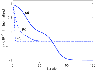
Abbildung 4: (Colour online) Gradient-flow driven local inversion of different Heisenberg interaction Hamiltonians: (a) the $ZZ$ interaction on a cyclic four-qubit topology $C_{4}$ can be locally inverted, (b) the $ZZ$ interaction on a cyclic three-qubit topology $C_{3}$ cannot be inverted locally, (c) nor the $XXX$ isotropic interaction between two qubits.

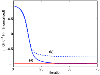
Abbildung 5: (Colour online) Gradient-flow driven local inversion of Heisenberg interactions of different quantum order on a cyclic three-qubit topology $C_{3}$: (a) the double-quantum interaction $X(-X)$ can be locally inverted, while (b) the zero-quantum analogue $XX$ cannot.

In the present context notice the gradient flow on the local unitaries takes the form

$$\begin{split}\dot{K}\,=\,\operatorname{grad}f(K)&=P_{\mathfrak{k}}([(KHK^{-1}),H])\;K\\[5.69054pt] &=-P_{\mathfrak{k}}\big{(}\operatorname{ad_{H}}\;\circ\;\operatorname{Ad_{K}}(H)\,\big{)}\;K\;,\end{split}$$ (65)

where $P_{\mathfrak{k}}$ denotes the projection onto the subalgebra $\mathfrak{k}$ of generators of local unitaries ${\mathbf{K}}=\mathbf{SU}(2)^{\otimes n}$. The flow clearly reaches a critical point if already the entire commutator vanishes

$$[\operatorname{Ad_{K}}(H),H]=0\quad.$$ (66)

For hermitian $H$, this is the case, for instance whenever

$$\operatorname{Ad_{K}}(H)=e^{\pm ip\pi}\;H\quad\text{(with $p=0,1,2,\dots$)}\quad,$$ (67)

which means $H$ is an eigenoperator to $\operatorname{Ad_{K}}(H)$, i.e., ${\rm vec}\,H$ is an eigenvector of $(K^{*}\,\otimes K)$. Eigenvectors $H$ to the eigenvalue $+1$ lead to global minima of $f(K)$, while global maxima are reached by eigenvectors $H$ to the eigenvalue $-1$.

In Figs. 4 and 5, we give some examples. Let $H$ be normalised to ${||H||}_{2}=1$. If $\operatorname{tr}\{KHK^{-1}H\}=-1$ can be reached, the interaction Hamiltonian is locally invertible as in the case of the Heisenberg $ZZ$ interaction in a cyclic four-qubit coupling topology (which clearly is a bipartite graph), while in the cyclic three-qubit topology (obviously not forming a bipartite coupling graph) or in the case of the isotropic $XXX$ interaction it is not.

Relation to Local $C$-Numerical Ranges

The $C$-numerical range is well-known Li (1994) to consist of the following set of points in the complex plane

$$W(C,A):=\{\operatorname{tr}\,(C^{\dagger}UAU^{-1})\;|\;U\in SU(2^{n})\}\;.$$ (68)

In Ref. Dirr et al. (2006), we defined as local $C$-numerical range its subset

$$W_{\rm{loc}}(C,A):=\{\operatorname{tr}\,(C^{\dagger}KAK^{-1})\;|\;K\in SU(2)^{\otimes n}\}\;.$$ (69)

In view of locally reversible Hamiltonians, things specialise to $C=-H=-A$. Normalising again to $\|H\|{}=1$, a locally reversible Hamiltonian $H$ clearly requires $-1\in W_{\rm{loc}}(-H,H)$. This has just been exemplified by the numerical examples in the previous section. Moreover, being a linear map of the local unitary orbit, the local $C$-numerical range is connected. For locally reversible $H$, one finds the real line segment $[-1;+1]=W_{\rm{loc}}(-H,H)$, whereas in Hamiltonians that fail to be locally reversible, the line segment falls short of extending from $+1$ (which trivially always can be attained) to $-1$.

With these observations, the different aspects may be summed up.

Synopsis on Type-I Inversion

Corollary 3 (Local Time Reversal)

For an interaction Hamiltonian $H=H^{\dagger}$ with $\|H\|{}_{2}^{\phantom{2}}=1$ the following are equivalent:

1. $H$ is locally sign-reversible of type-I;

2. its local $C$-numerical range comprises $-1$:   $-1\in W_{\rm loc}(-H,H)$ ;

3. its local $C$-numerical range is the real line segment from $-1$ to $+1$:   $W_{\rm loc}(-H,H)\;=\;[-1\,;\,+1]$;

4. $\exists K\in SU(2)^{\otimes n}:$
     $\|KHK^{-1}+H\|{}_{2}^{2}=0\;\Leftrightarrow\;\operatorname{Ad}_{K}(H)=-H$

5. $H$ is locally unitarily similar to a $\bar{H\;}$ with
   $\operatorname{Ad}_{K_{z}}(\bar{H\;})=-\bar{H\;}$;

6. let $\mathfrak{g}=\mathfrak{g}_{0}\oplus\;\bigoplus\limits_{i\neq j}\mathbb{C}^{\,}{}E_{ij}$ be the root-space decomposition of $\mathfrak{sl}(N,\mathbb{C}^{\,}{})$; $H$ is locally unitarily similar to a linear combination of root-space elements to non-zero roots

   $$\bar{H\;}:=\sum\limits_{\lambda=1}^{m}c_{\lambda}E_{ij}^{(\lambda)}$$

   satisfying a system of linear equations

   $$\sum_{\ell}p_{\lambda,\ell}\cdot\phi_{\ell}=\pm\pi(\operatorname{mod}{\;}2\pi)$$

   in the sense of Eqn. 40, where the $p_{\lambda,\ell}$ can be interpreted as the quantum orders of the constituting spherical tensor elements.

Proof: The equivalence of (1) with statements (2) through (6) was of course already proven in the respective sections.
Moreover, one finds (1) $\Rightarrow$ (2): obvious; (2) $\Rightarrow$ (3): connectedness of $W_{\rm loc}(C,A)$; (3) $\Rightarrow$ (4): obvious; (4) $\Rightarrow$ (5): Corollary 1; (5) $\Rightarrow$ (6): Corollary 1, Proposition 1 and 2; as well as Corollary 2 for the interpretation as quantum orders; (6) $\Rightarrow$ (1): Proposition 2. $\blacksquare$

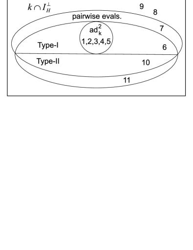
Abbildung 6: Venn diagram showing that simple criteria of non-zero eigenvalues in pairs of opposite sign, $\operatorname{ad}_{k}^{2}(H)=H$, and $I_{H}^{\perp}\cap\mathfrak{k}\neq\{\}$ fail to decide type-I invertibility as explained in the text. The numbers in the sets refer to the examples listed in Tab. 5.

However, the simple necessary criteria of (i) non-zero eigenvalues occuring in pairs of opposite sign, (ii) the intersection of the orthocomplement to the invariant subspace with the generators of local unitaries not being empty $I_{H}^{\perp}\cap\mathfrak{k}\neq\{\}$, as well as the sufficient condition (iii) of the double commutator reproducing the Hamiltonian in question, $\operatorname{ad}_{k}^{2}(H)=H$, fall short of giving a conclusive decision on type-I invertibility, see Fig. 6.

II Pointwise Locally Invertible Propagators

Tabelle 5: Examples of pair interaction and multi-qubit interaction Hamiltonians used to show the coverage by simple type-I inversion criteria in Fig. 6.

Example	Hamiltonian
1	$zz$
2	$xx+yy$
3	$xx1-yy1+x1x$
	$-y1y+1xx-1yy$
4	$xx11-yy11-1xxx+1yxy+1yyx+1xyy$
	$-x1xx+y1xy+y1yx+x1yy$
5	$xx11-yy11+x111-1xxx+1yxy+1yyx+1xyy$
	$-x1xx+y1xy+y1yx+x1yy$
6	$z11-xxx+xyy+yxy+yyx$
7	$xx1+yy1+zz1$
	$-(1xx+1yy+1zz)$
8	$xx1+yy1+x1x$
	$+y1y+1xx+1yy$
9	$zz1+z1z+1zz$
10	$zz+z1+1x$
11	$zz+z1+1z$

Propagators that are not jointly invertible by a local unitary for all $t\in\mathbb{R}^{\,}{}$ (together with the entire one-parameter group generated by their Hamiltonian) may still be pointwise locally invertible at certain times $\tau$. So the task in this section is the following: given some $\tau>0$, determine whether there is a pair $\{K_{1},K_{2}\neq K_{1}^{-1}\}\subset\mathbf{K}:=\mathbf{SU}(2)^{\otimes n}\;$ so that

$$\begin{split}K_{1}\;e^{-i\tau H}\;K_{2}&=e^{+i\tau H}\\ \Leftrightarrow\;(K_{2}^{t}\otimes K_{1}^{\phantom{t}})\;\operatorname{vec}(e^{-i\tau H})&=\operatorname{vec}(e^{+i\tau H})\;.\end{split}$$ (70)

Remark 2

Note that type-II invertibility only arises upon restriction to local operations $K_{1},K_{2}\in\mathbf{K}$, because to any $U_{0}\in\mathbf{SU}(N)$ there is a trivial pair $U_{1},U_{2}\in\mathbf{SU}(N)$ with $U_{1}U_{0}U_{2}=U_{0}^{-1}$ (e.g. $U_{1}=U_{0}^{-2},U_{2}={\rm 1\negthickspace l}{}$), whereas with $K_{1},K_{2}\in\mathbf{K}$ there is no such trivial generic solution unless $U_{0}\in\mathbf{K}$.

Corollary 4

Let $H$ generate a one-parameter unitary group $\mathcal{U}:=\{e^{-it\,H}\,|\,t\in\mathbb{R}^{\,}{},iH\in\mathfrak{su}(N,\mathbb{C}^{\,}{})\}$ that is locally invertible of type-I. Then

1. the generic elements of the left and right cosets $\mathbf{K}\mathcal{U}$ and $\mathcal{U}\mathbf{K}$ are type-II locally invertible;

2. in turn, every Hamiltonian that is type-II invertible is an element of a coset $\mathbf{K}\mathcal{U}$ or $\mathcal{U}\mathbf{K}$, where $\mathcal{U}$ is some one-parameter unitary group that itself is type-I invertible.

Therefore type-II invertible propagators are a natural extension of the type-I invertible unitary one-parameter groups. In turn, however, the decision problem whether a given propagator is type-II invertible is generally quite complicated so that we will devise a coupled gradient flow on two local unitaries for solving it numerically. Yet a number of cases can be treated algebraically by analysing the symmetries of the matrix representation of the unitary propagator to be inverted.

Since these symmetry considerations extend beyond the representation of unitary matrices, we will ask whether an arbitrary given matrix can be mapped to its hermitian adjoint by a superoperator of the form $(K_{2}^{t}\otimes K_{1}^{\phantom{t}})$ with local unitary $K_{1},K_{2}$ (cp. Eqn. 70). To this end, one has to maximise the coincidences between $(K_{2}^{t}\otimes K_{1}^{\phantom{t}})$ and the adjoining superoperator denoted $\widehat{\operatorname{Adj}}{}$ that takes its argument to the hermitian adjoint (i.e. the complex conjugate transpose). Clearly, there is no local unitary $(K_{2}^{t}\otimes K_{1}^{\phantom{t}})$ that fully matches with $\widehat{\operatorname{Adj}}{}$ as this would be a universal inverting operator. However, there are classes of partial overlaps, where the lack of coincidence enforces a symmetry in the matrices to be adjoined. These will be analysed in detail in the following.

Because $\widehat{\operatorname{Adj}}{}$ has no matrix representation over the field of complex numbers, we turn to the real domain. With $M_{\operatorname{Re}}$ and $M_{\operatorname{Im}}$ denoting the respective real and imaginary parts of an arbitrary complex matrix $M$, one obtains a convenient representation of $M$ as a real vector by virtue of the faithful mapping

$$M\mapsto\operatorname{vec}(M_{\operatorname{Re}})\oplus\operatorname{vec}(M_{\operatorname{Im}})\;.$$ (71)

[Note that this representation shows less redundance than the usual $M\mapsto\left(\begin{smallmatrix}M_{\operatorname{Re}}\;-M_{\operatorname{Im}}\\ M_{\operatorname{Im}}\;\phantom{-}M_{\operatorname{Re}}\end{smallmatrix}\right)$.]

In this notation, the adjoining superoperator does have a real matrix representation defined via

$$\widehat{\operatorname{Adj}{}}_{\mathbb{R}}^{\,}{}\big{(}\operatorname{vec}(M_{\operatorname{Re}})\oplus\operatorname{vec}(M_{\operatorname{Im}})\big{)}=\operatorname{vec}(M_{\operatorname{Re}}^{t})\oplus\operatorname{vec}(-M_{\operatorname{Im}}^{t})$$ (72)

such as to take the form

$$\widehat{\operatorname{Adj}}{}_{\mathbb{R}^{\,}{}}=\left(\begin{smallmatrix}\widehat{T}&\phantom{-}\widehat{0}\\[2.84526pt] \widehat{0}&-\widehat{T}\end{smallmatrix}\right)\quad,$$ (73)

by virtue of the transposition superoperator $\widehat{T}$, which e.g. for the above representation of a $M\in\operatorname{Mat}{}_{4}(\mathbb{C}^{\,}{})$ reads

$$\widehat{T}:=\left(\,\setcounter{MaxMatrixCols}{16}\begin{smallmatrix}1&\cdot&\cdot&\cdot&\cdot&\cdot&\cdot&\cdot&\cdot&\cdot&\cdot&\cdot&\cdot&\cdot&\cdot&\cdot\\ \cdot&\cdot&\cdot&\cdot&1&\cdot&\cdot&\cdot&\cdot&\cdot&\cdot&\cdot&\cdot&\cdot&\cdot&\cdot\\ \cdot&\cdot&\cdot&\cdot&\cdot&\cdot&\cdot&\cdot&1&\cdot&\cdot&\cdot&\cdot&\cdot&\cdot&\cdot\\ \cdot&\cdot&\cdot&\cdot&\cdot&\cdot&\cdot&\cdot&\cdot&\cdot&\cdot&\cdot&1&\cdot&\cdot&\cdot\\ \cdot&1&\cdot&\cdot&\cdot&\cdot&\cdot&\cdot&\cdot&\cdot&\cdot&\cdot&\cdot&\cdot&\cdot&\cdot\\ \cdot&\cdot&\cdot&\cdot&\cdot&1&\cdot&\cdot&\cdot&\cdot&\cdot&\cdot&\cdot&\cdot&\cdot&\cdot\\ \cdot&\cdot&\cdot&\cdot&\cdot&\cdot&\cdot&\cdot&\cdot&1&\cdot&\cdot&\cdot&\cdot&\cdot&\cdot\\ \cdot&\cdot&\cdot&\cdot&\cdot&\cdot&\cdot&\cdot&\cdot&\cdot&\cdot&\cdot&\cdot&1&\cdot&\cdot\\ \cdot&\cdot&1&\cdot&\cdot&\cdot&\cdot&\cdot&\cdot&\cdot&\cdot&\cdot&\cdot&\cdot&\cdot&\cdot\\ \cdot&\cdot&\cdot&\cdot&\cdot&\cdot&1&\cdot&\cdot&\cdot&\cdot&\cdot&\cdot&\cdot&\cdot&\cdot\\ \cdot&\cdot&\cdot&\cdot&\cdot&\cdot&\cdot&\cdot&\cdot&\cdot&1&\cdot&\cdot&\cdot&\cdot&\cdot\\ \cdot&\cdot&\cdot&\cdot&\cdot&\cdot&\cdot&\cdot&\cdot&\cdot&\cdot&\cdot&\cdot&\cdot&1&\cdot\\ \cdot&\cdot&\cdot&1&\cdot&\cdot&\cdot&\cdot&\cdot&\cdot&\cdot&\cdot&\cdot&\cdot&\cdot&\cdot\\ \cdot&\cdot&\cdot&\cdot&\cdot&\cdot&\cdot&1&\cdot&\cdot&\cdot&\cdot&\cdot&\cdot&\cdot&\cdot\\ \cdot&\cdot&\cdot&\cdot&\cdot&\cdot&\cdot&\cdot&\cdot&\cdot&\cdot&1&\cdot&\cdot&\cdot&\cdot\\ \cdot&\cdot&\cdot&\cdot&\cdot&\cdot&\cdot&\cdot&\cdot&\cdot&\cdot&\cdot&\cdot&\cdot&\cdot&1\\ \\ \end{smallmatrix}\,\right)\quad.$$ (74)

Likewise, for the local unitary transform $K_{1}MK_{2}\;{\widehat{=}}\;\widehat{K}\operatorname{vec}(M)$ with $\widehat{K}:=K_{2}^{t}\otimes K_{1}^{\phantom{t}}$ one gets the corresponding real representation of the superoperator via

$$\widehat{K}_{\mathbb{R}^{\,}{}}\operatorname{vec}(M)_{\mathbb{R}^{\,}{}}:=\left(\begin{smallmatrix}\widehat{K}_{\operatorname{Re}}&-\widehat{K}_{\operatorname{Im}}\\[2.84526pt] \widehat{K}_{\operatorname{Im}}&{\phantom{-}}\widehat{K}_{\operatorname{Re}}\end{smallmatrix}\right)\big{(}\operatorname{vec}(M_{\operatorname{Re}})\oplus\operatorname{vec}(M_{\operatorname{Im}})\big{)}\;.$$ (75)

Comparing the structure of $\widehat{K}_{\mathbb{R}^{\,}{}}$ here and $\widehat{\operatorname{Adj}}{}_{\mathbb{R}^{\,}{}}$ (in Eqn. 73) immediately shows that for maximal coincidence the imaginary block $\widehat{K}_{\operatorname{Im}}$ within $\widehat{K}_{\mathbb{R}^{\,}{}}$ has to vanish, because the row and column norms are limited to unity in (local) unitaries. One may readily express the utmost possible overlaps of $\widehat{K}_{\mathbb{R}^{\,}{}}$ and $\widehat{\operatorname{Adj}}{}_{\mathbb{R}^{\,}{}}$ by taking the elementwise Hadamard product as the coincidence matrix $\widehat{C}$

$$\begin{split}\widehat{C}_{\mathbb{R}^{\,}{}}:&=\widehat{K}_{\mathbb{R}^{\,}{}}\odot\widehat{\operatorname{Adj}}{}_{\mathbb{R}^{\,}{}}\\[8.53581pt] &=\left(\begin{smallmatrix}\widehat{K}_{\operatorname{Re}}&-\widehat{K}_{\operatorname{Im}}\\[2.84526pt] \widehat{K}_{\operatorname{Im}}&{\phantom{-}}\widehat{K}_{\operatorname{Re}}\end{smallmatrix}\right)\odot\left(\begin{smallmatrix}\widehat{T}&{\phantom{-}}\widehat{0}\\[2.84526pt] \widehat{0}&-\widehat{T}\end{smallmatrix}\right)\\[8.53581pt] &=\left(\begin{smallmatrix}\widehat{C}&\phantom{-}\widehat{0}\\[2.84526pt] \widehat{0}&-\widehat{C}\end{smallmatrix}\right)\;,\end{split}$$ (76)

where $\widehat{C}$ reads, e.g. in the case $n=4$

$$\widehat{C}:=\pm\small\left(\setcounter{MaxMatrixCols}{16}\begin{smallmatrix}+a&\cdot&\cdot&\cdot&\cdot&\cdot&\cdot&\cdot&\cdot&\cdot&\cdot&\cdot&\cdot&\cdot&\cdot&\cdot\\ \cdot&\cdot&\cdot&\cdot&\pm b&\cdot&\cdot&\cdot&\cdot&\cdot&\cdot&\cdot&\cdot&\cdot&\cdot&\cdot\\ \cdot&\cdot&\cdot&\cdot&\cdot&\cdot&\cdot&\cdot&\pm c&\cdot&\cdot&\cdot&\cdot&\cdot&\cdot&\cdot\\ \cdot&\cdot&\cdot&\cdot&\cdot&\cdot&\cdot&\cdot&\cdot&\cdot&\cdot&\cdot&+d&\cdot&\cdot&\cdot\\ \cdot&+b&\cdot&\cdot&\cdot&\cdot&\cdot&\cdot&\cdot&\cdot&\cdot&\cdot&\cdot&\cdot&\cdot&\cdot\\ \cdot&\cdot&\cdot&\cdot&\cdot&\pm a&\cdot&\cdot&\cdot&\cdot&\cdot&\cdot&\cdot&\cdot&\cdot&\cdot\\ \cdot&\cdot&\cdot&\cdot&\cdot&\cdot&\cdot&\cdot&\cdot&\pm d&\cdot&\cdot&\cdot&\cdot&\cdot&\cdot\\ \cdot&\cdot&\cdot&\cdot&\cdot&\cdot&\cdot&\cdot&\cdot&\cdot&\cdot&\cdot&\cdot&+c&\cdot&\cdot\\ \cdot&\cdot&+c&\cdot&\cdot&\cdot&\cdot&\cdot&\cdot&\cdot&\cdot&\cdot&\cdot&\cdot&\cdot&\cdot\\ \cdot&\cdot&\cdot&\cdot&\cdot&\cdot&\pm d&\cdot&\cdot&\cdot&\cdot&\cdot&\cdot&\cdot&\cdot&\cdot\\ \cdot&\cdot&\cdot&\cdot&\cdot&\cdot&\cdot&\cdot&\cdot&\cdot&\pm a&\cdot&\cdot&\cdot&\cdot&\cdot\\ \cdot&\cdot&\cdot&\cdot&\cdot&\cdot&\cdot&\cdot&\cdot&\cdot&\cdot&\cdot&\cdot&\cdot&+b&\cdot\\ \cdot&\cdot&\cdot&+d&\cdot&\cdot&\cdot&\cdot&\cdot&\cdot&\cdot&\cdot&\cdot&\cdot&\cdot&\cdot\\ \cdot&\cdot&\cdot&\cdot&\cdot&\cdot&\cdot&\pm c&\cdot&\cdot&\cdot&\cdot&\cdot&\cdot&\cdot&\cdot\\ \cdot&\cdot&\cdot&\cdot&\cdot&\cdot&\cdot&\cdot&\cdot&\cdot&\cdot&\pm b&\cdot&\cdot&\cdot&\cdot\\ \cdot&\cdot&\cdot&\cdot&\cdot&\cdot&\cdot&\cdot&\cdot&\cdot&\cdot&\cdot&\cdot&\cdot&\cdot&+a\\ \\ \end{smallmatrix}\right)$$ (77)

and in which either $a$ or $b$ or $c$ or $d$ is unity. Thus in the case $n=4$ one finds four subtypes of maximal overlap, termed $A,B,C,D$ henceforth. According to the possible choices of signs, each of them occurs in four sign patterns expressed by the indices $\nu\in\{A_{++++},A_{+--+},A_{-++-},A_{----}\}$ and analogously for subtypes $B,C,D$.

For instance, let $\nu=A_{+--+}$, then the local unitary $\widehat{K}_{\mathbb{R}^{\,}{}}$ for maximal overlap with $\widehat{\operatorname{Adj}}{}_{\mathbb{R}^{\,}{}}$ shows the following non-zero block $\widehat{K}_{\operatorname{Re}}$:

$$\widehat{K}_{\operatorname{Re}}^{(A_{+--+})}=\left(\setcounter{MaxMatrixCols}{16}\begin{smallmatrix}\\ {\color[rgb]{1,0,0}+}&\cdot&\cdot&\cdot&\cdot&\cdot&\cdot&\cdot&\cdot&\cdot&\cdot&\cdot&\cdot&\cdot&\cdot&\cdot\\ \cdot&\star&\cdot&\cdot&\cdot&\cdot&\cdot&\cdot&\cdot&\cdot&\cdot&\cdot&\cdot&\cdot&\cdot&\cdot\\ \cdot&\cdot&\star&\cdot&\cdot&\cdot&\cdot&\cdot&\cdot&\cdot&\cdot&\cdot&\cdot&\cdot&\cdot&\cdot\\ \cdot&\cdot&\cdot&\star&\cdot&\cdot&\cdot&\cdot&\cdot&\cdot&\cdot&\cdot&\cdot&\cdot&\cdot&\cdot\\ \cdot&\cdot&\cdot&\cdot&\star&\cdot&\cdot&\cdot&\cdot&\cdot&\cdot&\cdot&\cdot&\cdot&\cdot&\cdot\\ \cdot&\cdot&\cdot&\cdot&\cdot&{\color[rgb]{1,0,0}-}&\cdot&\cdot&\cdot&\cdot&\cdot&\cdot&\cdot&\cdot&\cdot&\cdot\\ \cdot&\cdot&\cdot&\cdot&\cdot&\cdot&\star&\cdot&\cdot&\cdot&\cdot&\cdot&\cdot&\cdot&\cdot&\cdot\\ \cdot&\cdot&\cdot&\cdot&\cdot&\cdot&\cdot&\star&\cdot&\cdot&\cdot&\cdot&\cdot&\cdot&\cdot&\cdot\\ \cdot&\cdot&\cdot&\cdot&\cdot&\cdot&\cdot&\cdot&\star&\cdot&\cdot&\cdot&\cdot&\cdot&\cdot&\cdot\\ \cdot&\cdot&\cdot&\cdot&\cdot&\cdot&\cdot&\cdot&\cdot&\star&\cdot&\cdot&\cdot&\cdot&\cdot&\cdot\\ \cdot&\cdot&\cdot&\cdot&\cdot&\cdot&\cdot&\cdot&\cdot&\cdot&{\color[rgb]{1,0,0}-}&\cdot&\cdot&\cdot&\cdot&\cdot\\ \cdot&\cdot&\cdot&\cdot&\cdot&\cdot&\cdot&\cdot&\cdot&\cdot&\cdot&\star&\cdot&\cdot&\cdot&\cdot\\ \cdot&\cdot&\cdot&\cdot&\cdot&\cdot&\cdot&\cdot&\cdot&\cdot&\cdot&\cdot&\star&\cdot&\cdot&\cdot\\ \cdot&\cdot&\cdot&\cdot&\cdot&\cdot&\cdot&\cdot&\cdot&\cdot&\cdot&\cdot&\cdot&\star&\cdot&\cdot\\ \cdot&\cdot&\cdot&\cdot&\cdot&\cdot&\cdot&\cdot&\cdot&\cdot&\cdot&\cdot&\cdot&\cdot&\star&\cdot\\ \cdot&\cdot&\cdot&\cdot&\cdot&\cdot&\cdot&\cdot&\cdot&\cdot&\cdot&\cdot&\cdot&\cdot&\cdot&{\color[rgb]{1,0,0}+}\\ \\ \end{smallmatrix}\right)\;,$$ (78)

where the elements $\pm$ stand for $\pm 1$, while $*$ are unavoidable non-zero elements enforced by $\widehat{K}_{\mathbb{R}^{\,}{}}$ being a local unitary. They do not contribute to $\widehat{\operatorname{Adj}}{}_{\mathbb{R}^{\,}{}}$, in contrary, they bring about unwanted actions on the argument, i.e. the matrix $M\in\operatorname{Mat}{}_{n}(\mathbb{C}^{\,}{})$. Together with the lacking elements for full overlap with $\widehat{T}$, they require the following symmetry in the matrix argument

$$M_{A_{+--+}}=\left(\begin{smallmatrix}\\ M_{11}^{\operatorname{Re}}&0&0&M_{14}\\ 0&M_{22}^{\operatorname{Im}}&M_{23}&0\\ 0&\pm M_{23}^{*}&M_{33}^{\operatorname{Im}}&0\\ \mp M_{14}^{*}&0&0&M_{44}^{\operatorname{Re}}\\ \end{smallmatrix}\right)$$ (79)

in order to fulfill $\widehat{K}_{\mathbb{R}^{\,}{}}\operatorname{vec}(M)=\operatorname{vec}(M^{\dagger})$ as desired.

For the sake of completeness in the case of $n=4$, we give the remainder of constituents in the subtypes $A,B,C,D$ as well as the associated sign patterns in Appendix-C and D.

The structures of the pertinent block matrices $\widehat{T}$, $\widehat{\operatorname{Adj}}{}_{\mathbb{R}^{\,}{}}$ and hence $\widehat{C}$ are easily scalable to larger $n$: in Tab. 6 we give the number of subtypes of coincidence as well as the number of different symmetry subtypes and sign patterns in the matrix arguments $M\in\operatorname{Mat}{}_{n}(\mathbb{C}^{\,}{})$ with growing number of dimensions.

Tabelle 6: Subtypes and Sign Patterns in Type-II Inversion

$\#$ spin qubits		$\#$ subtypes		$\#$ sign patterns
$2$		$4$		$4$
$3$		$8$		$8$
$\vdots$		$\vdots$		$\vdots$
$n$		$2^{n}$		$2^{n}$

Type-II Inversion via Coupled Gradient Flows on Two Local Unitaries

In the general case, one may conveniently restate the problem of pointwise local invertibility to the question, whether for a fixed non-zero $\tau\in\mathbb{R}^{\,}{}$ there is a pair $K_{1},K_{2}\in{\mathbf{K}}=SU(2)^{\otimes n}$ so that

$$\begin{split}K_{1}e^{-i\tau H}K_{2}&=e^{+i\tau H}\\ \Leftrightarrow||K_{1}e^{-i\tau H}K_{2}-e^{+i\tau H}||_{2}&=0\quad.\end{split}$$ (80)

Then one may devise a coupled gradient flow on two local unitaries simultaneously in order to minimise

$$f(K_{1},K_{2})=\operatorname{Re}\;\operatorname{tr}\{K_{1}e^{-i\tau H}K_{2}(-e^{-i\tau H})\}$$ (81)

by (writing $U:=e^{-i\tau H}$ for short)

$$\dot{K}_{1} = \operatorname{grad}f(K_{1})=P_{\mathfrak{k}}\,\big{(}K_{1}UK_{2}(-U)\big{)}\;K_{1}$$ (82)

$$\dot{K}_{2} = \operatorname{grad}f(K_{2})=P_{\mathfrak{k}}\,\big{(}K_{2}(-U)K_{1}U\big{)}\;K_{2}\quad.$$ (83)

Again, if $\tfrac{1}{N}\;\operatorname{Re}\;\operatorname{tr}\{K_{1}e^{-i\tau H}K_{2}(-e^{-i\tau H})\}=-1$ can be reached, then $U(\tau)=e^{-i\tau H}$ is locally invertible at the point $\tau$. Examples are shown in Fig. 7.

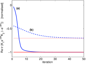
Abbildung 7: (Colour online) Gradient-flow driven local inversion of $U(t):=\exp\{-i\tfrac{\pi}{4}\;H\}$ with $H=(\sigma_{z}\otimes{\rm 1\negthickspace l}{}+{\rm 1\negthickspace l}{}\otimes\sigma_{z}+\sigma_{z}\otimes\sigma_{z})/2$
(a) by coupled gradient flows on independent $K_{1}$ and $K_{2}$ and (b) by a gradient flow with $K_{2}^{\phantom{1}}=K_{1}^{-1}$.

Conclusion

Generalising in the sense of Hahn’s spin echo, we have characterised all those effective multi-qubit quantum interactions allowing for time reversal by manipulations confined to local unitary operations. The evolutions generated by these interaction Hamiltonians can be reversed and refocussed solely by local unitaries. To this end, we have given a number of necessary and sufficient conditions in terms of geometry, eigenoperators, graphs of coupling topology, tensor analysis and root-space decomposition. Moreover, we have classified locally invertible evolutions into two types. Type-I consists of one-parameter groups generated by Hamiltonians $H$ that are eigenoperators of local unitary conjugation associated with the eigenvalue $-1$, i.e. $\operatorname{Ad}_{K}(H)=-H$. We have shown how to construct the corresponding eigenspace in closed algebraic form. Hamiltonians generating type-I invertible evolutions are locally unitarily similar to those invertible solely by local $z$-rotations, which thus can be regarded as normal form. Taking the differential, we showed their components $E_{ij}$ relate to the non-zero roots of the root-space decomposition of $\mathfrak{sl}(N,\mathbb{C}^{\,}{})$ via $\operatorname{ad}_{k_{z}}(E_{ij})=(e_{i}-e_{j})(E_{ij})$, where $k_{z}$ are the generators of local $z$-rotations. Moreover, in the special case of joint local $z$-rotations generated by $F_{z}$, the non-zero roots were further shown to relate to the spherical tensors $T_{j,p}$ of non-zero quantum order $p$. For Ising ZZ-coupling interactions as well as for Heisenberg $XY$ interactions to be locally invertible of type-I, their coupling topology has to take the form of a bipartite graph. An exception is the Heisenberg $X(-X)$ interaction, which is type-I invertible on any coupling topology, while Heisenberg $XXX$, $XXY$, and $XYZ$ interactions are not locally invertible at all because they relate to rank-$0$ tensors, and their non-zero eigenvalues do not occur in pairs of opposite sign.

The pointwise invertible quantum evolutions of type-II are generalisations of those of type-I. They consist of coset elements $\mathbf{K}\mathcal{U}$ and $\mathcal{U}\mathbf{K}$, where $\mathcal{U}$ are type-I invertible one-parameter groups. Here we have caracterised type-II invertible propagators by the symmetries of their matrix representations.

Finally, in view of convenience in practical applications, we have devised gradient-flow based numerical checks to decide whether

$$\underset{K_{1},K_{2}\in SU(2)^{\otimes n}}{\min}\|K_{1}e^{-itH}K_{2}-e^{+itH}\|{}^{2}_{2}=0\;,$$

i.e. whether a propagator is locally invertible of type-I or type-II or not.

III Appendix

III.1 Classification

First, we prove Lemma 0 from the introduction:
Either $e^{-itH}$ is

1. not invertible by local unitaries at all, or

2. it is trivial and self-inverse, or

3. it is type-I invertible in the sense $\exists K\in SU(2)^{\otimes n}:KHK^{-1}=-H$ so $Ke^{-itH}K^{-1}=e^{+itH}$ jointly for all $t\in\mathbb{R}^{\,}{}$, or

4. it is type-II invertible such that at some (but not all) points $\tau$ in time $K_{1}e^{-i\tau H}K_{2}=e^{+i\tau H}$ with $K_{1},K_{2}\in SU(2)^{\otimes n}$ and $K_{2}^{\phantom{1}}\neq K_{1}^{-1}$.

Proof: By the series expansion of the exponential one finds the obvious equivalence

$$\begin{split}KHK^{-1}&=-H\\ &\Leftrightarrow\forall t\in\mathbb{R}^{\,}{}:Ke^{-itH}K^{-1}=e^{+itH}.\end{split}$$ (84)

Its logical negation

$$\begin{split}KHK^{-1}&\neq-H\\ &\Leftrightarrow\exists t\in\mathbb{R}^{\,}{}:Ke^{-itH}K^{-1}\neq e^{+itH},\end{split}$$ (85)

comprises the following trivial cases

1. $\forall t\in\mathbb{R}^{\,}{}:Ke^{-itH}K^{-1}\neq e^{+itH}$, so either $e^{-itH}$ is not locally invertible at all, or

2. $\exists\tau\neq 0:Ke^{-i\tau H}K^{-1}=e^{+i\tau H}$, while for all other $t\neq\tau$ (with exceptions of measure zero due to periodicity) $Ke^{-itH}K^{-1}\neq e^{+itH}$ while $(KHK^{-1})\neq-H$. This can only hold, if $K={\rm 1\negthickspace l}{}$ and $e^{-i\tau H}$ is self-inverse.

Otherwise, if the affirmative (Eqn 84) is true one has

1. $\forall t\in\mathbb{R}^{\,}{}:Ke^{-itH}K^{-1}=e^{+itH}$.

Finally, we have to show that type-I and II are distinct

1. $K_{1}e^{-i\tau H}K_{2}=e^{+i\tau H}$ with $K_{1}^{\phantom{1}}\neq K_{2}^{-1}$ may hold pointwise for certain $\tau$, but not for all $\tau\in\mathbb{R}^{\,}{}$. Assume the contrary: $\forall t\in\mathbb{R}^{\,}{}$ $K_{1}e^{-itH}K_{2}=e^{+itH}$ with $K_{1}^{\phantom{1}}\neq K_{2}^{-1}$ and define as commuting elements of a one-parameter group $U_{1}:=e^{-it_{1}H}$ and $U_{2}:=e^{-it_{2}H}$ to give $U_{12}:=e^{-i(t_{1}+t_{2})H}$. Then one has

   $$K_{1}U_{12}K_{2} = U_{12}^{-1}$$

   $$K_{1}U_{1}U_{2}K_{2} = U_{2}^{-1}U_{1}^{-1}=U_{1}^{-1}U_{2}^{-1}$$

   $$(K_{1}U_{1}K_{2})(\underline{K_{2}^{-1}}U_{2}^{\phantom{1}}K_{2}^{\phantom{1}}) = (K_{1}U_{1}K_{2})(\underline{K_{1}}U_{2}K_{2})$$

   $$K_{2}^{-1} = K_{1}^{\phantom{1}}\quad,$$

   where the latter contradicts the assumption.

These four instances prove Tab. 1. $\hfill\blacksquare$

III.2 Explicit General Representation of $F_{z}$

Recall that the generator of a joint $z$-rotation on all the $n$ spin-$\tfrac{1}{2}$ qubits is defined as the diagonal matrix

$$F_{z}:=\tfrac{1}{2}\sum\limits_{\ell=1}^{n}{\rm 1\negthickspace l}{}^{(1)}\otimes{\rm 1\negthickspace l}{}^{(2)}\otimes\cdots\otimes{\rm 1\negthickspace l}{}^{(\ell-1)}\otimes\sigma_{z}^{(\ell)}\otimes{\rm 1\negthickspace l}{}^{(\ell+1)}\otimes\cdots\otimes{\rm 1\negthickspace l}{}^{(n)}$$ (86)

summing over the Pauli matrix $\sigma_{z}^{(\ell)}$ on all qubits. Whenever it is necessary to express the total number of qubits, we write $F_{z}^{n}$. Here we prove an explicit formula giving its $i^{\rm th}$ diagonal element for general $n$.

Lemma 8

For ${(F_{z}^{n})}_{ii}$ with the index $i\in\{1,2,3,\dots,2^{n}\}$ calculate the $n$-digit binary representation for the reduction by 1 as $(i-1)_{2}=:\sum_{k=0}^{n-1}2^{k}b_{k}$. Then the $i^{\rm th}$ diagonal element reads

$${(F_{z}^{n})}_{ii}=\tfrac{1}{2}\sum_{k=0}^{n-1}(-1)^{b_{k}}\quad.$$ (87)

Proof (induction):
For $n=1$ one has: $(i-1)_{2}=2^{0}b_{0}\in\{0,1\}$ so ${(F_{z}^{1})}_{ii}=\frac{1}{2}\sum_{k=0}^{(1-1)}(-1)^{b_{k}}$ giving ${(F_{z}^{1})}_{11}=\tfrac{1}{2}=-{(F_{z}^{1})}_{22}$.

In order to proceed from $n\rightarrow n+1$ we show that with ${(F_{z}^{n})}_{ii}$ being given one finds for the new index $i^{\prime}:=2^{n}b_{n}+i\in\{1,2,3,\dots,2^{n+1}\}$

$${(F_{z}^{n+1})}_{i^{\prime}i^{\prime}}=({\rm 1\negthickspace l}{}\otimes F_{z}^{n})_{i^{\prime}i^{\prime}}+\tfrac{1}{2}(-1)^{b_{n}}\quad.$$ (88)

Use

$$\begin{split}F_{z}^{n+1}&={\rm 1\negthickspace l}{}_{2}\otimes F_{z}^{n}+I_{z}\otimes{\rm 1\negthickspace l}{}_{2^{n}}\\[5.69054pt] &=\operatorname{diag}{}\left({(F_{z}^{n})}_{11},\dots,{(F_{z}^{n})}_{2^{n}2^{n}};{(F_{z}^{n})}_{11},\dots,{(F_{z}^{n})}_{2^{n}2^{n}}\right)\\ &\phantom{XX}+\tfrac{1}{2}\operatorname{diag}{}(1,1,\dots,1;-1,-1,\dots,-1)\end{split}$$ (89)

to see that the last term adds $\tfrac{1}{2}$ for $i^{\prime}\in\{1,\dots,2^{n}\}=i$ and $-\tfrac{1}{2}$ for $i^{\prime}\in\{2^{n}+1,\dots,2^{n+1}\}=2^{n}+i$, in coincidence with $b_{n}$ taking the value $0$ or $1$. $\hfill\blacksquare$

III.3 Subtypes of Pointwise Invertible Local Unitaries

For the case of two qubits, we give local unitary superoperators of different type of partial overlap with the adjoining superoperator

$$\widehat{K}_{\mathbb{R}^{\,}{}}\operatorname{vec}(M)_{\mathbb{R}^{\,}{}}:=\left(\begin{smallmatrix}\widehat{K}_{\operatorname{Re}}&-\widehat{K}_{\operatorname{Im}}\\[2.84526pt] \widehat{K}_{\operatorname{Im}}&{\phantom{-}}\widehat{K}_{\operatorname{Re}}\end{smallmatrix}\right)\big{(}\operatorname{vec}(M_{\operatorname{Re}})\oplus\operatorname{vec}(M_{\operatorname{Im}})\big{)}\;.$$ (90)

In subtype $A$, the blockmatrix $\widehat{K}_{\operatorname{Re}}$ within the above supermatrix $\widehat{K}_{\mathbb{R}}^{\,}{}$ may take four different forms according to the indices

$$A_{++++}=-A_{----}=\left(\setcounter{MaxMatrixCols}{16}\begin{smallmatrix}\\ {\color[rgb]{1,0,0}+}&\cdot&\cdot&\cdot&\cdot&\cdot&\cdot&\cdot&\cdot&\cdot&\cdot&\cdot&\cdot&\cdot&\cdot&\cdot\\ \cdot&\star&\cdot&\cdot&\cdot&\cdot&\cdot&\cdot&\cdot&\cdot&\cdot&\cdot&\cdot&\cdot&\cdot&\cdot\\ \cdot&\cdot&\star&\cdot&\cdot&\cdot&\cdot&\cdot&\cdot&\cdot&\cdot&\cdot&\cdot&\cdot&\cdot&\cdot\\ \cdot&\cdot&\cdot&\star&\cdot&\cdot&\cdot&\cdot&\cdot&\cdot&\cdot&\cdot&\cdot&\cdot&\cdot&\cdot\\ \cdot&\cdot&\cdot&\cdot&\star&\cdot&\cdot&\cdot&\cdot&\cdot&\cdot&\cdot&\cdot&\cdot&\cdot&\cdot\\ \cdot&\cdot&\cdot&\cdot&\cdot&{\color[rgb]{1,0,0}+}&\cdot&\cdot&\cdot&\cdot&\cdot&\cdot&\cdot&\cdot&\cdot&\cdot\\ \cdot&\cdot&\cdot&\cdot&\cdot&\cdot&\star&\cdot&\cdot&\cdot&\cdot&\cdot&\cdot&\cdot&\cdot&\cdot\\ \cdot&\cdot&\cdot&\cdot&\cdot&\cdot&\cdot&\star&\cdot&\cdot&\cdot&\cdot&\cdot&\cdot&\cdot&\cdot\\ \cdot&\cdot&\cdot&\cdot&\cdot&\cdot&\cdot&\cdot&\star&\cdot&\cdot&\cdot&\cdot&\cdot&\cdot&\cdot\\ \cdot&\cdot&\cdot&\cdot&\cdot&\cdot&\cdot&\cdot&\cdot&\star&\cdot&\cdot&\cdot&\cdot&\cdot&\cdot\\ \cdot&\cdot&\cdot&\cdot&\cdot&\cdot&\cdot&\cdot&\cdot&\cdot&{\color[rgb]{1,0,0}+}&\cdot&\cdot&\cdot&\cdot&\cdot\\ \cdot&\cdot&\cdot&\cdot&\cdot&\cdot&\cdot&\cdot&\cdot&\cdot&\cdot&\star&\cdot&\cdot&\cdot&\cdot\\ \cdot&\cdot&\cdot&\cdot&\cdot&\cdot&\cdot&\cdot&\cdot&\cdot&\cdot&\cdot&\star&\cdot&\cdot&\cdot\\ \cdot&\cdot&\cdot&\cdot&\cdot&\cdot&\cdot&\cdot&\cdot&\cdot&\cdot&\cdot&\cdot&\star&\cdot&\cdot\\ \cdot&\cdot&\cdot&\cdot&\cdot&\cdot&\cdot&\cdot&\cdot&\cdot&\cdot&\cdot&\cdot&\cdot&\star&\cdot\\ \cdot&\cdot&\cdot&\cdot&\cdot&\cdot&\cdot&\cdot&\cdot&\cdot&\cdot&\cdot&\cdot&\cdot&\cdot&{\color[rgb]{1,0,0}+}\\ \\ \end{smallmatrix}\right)$$

$$A_{+--+}=-A_{-++-}=\left(\setcounter{MaxMatrixCols}{16}\begin{smallmatrix}\\ {\color[rgb]{1,0,0}+}&\cdot&\cdot&\cdot&\cdot&\cdot&\cdot&\cdot&\cdot&\cdot&\cdot&\cdot&\cdot&\cdot&\cdot&\cdot\\ \cdot&\star&\cdot&\cdot&\cdot&\cdot&\cdot&\cdot&\cdot&\cdot&\cdot&\cdot&\cdot&\cdot&\cdot&\cdot\\ \cdot&\cdot&\star&\cdot&\cdot&\cdot&\cdot&\cdot&\cdot&\cdot&\cdot&\cdot&\cdot&\cdot&\cdot&\cdot\\ \cdot&\cdot&\cdot&\star&\cdot&\cdot&\cdot&\cdot&\cdot&\cdot&\cdot&\cdot&\cdot&\cdot&\cdot&\cdot\\ \cdot&\cdot&\cdot&\cdot&\star&\cdot&\cdot&\cdot&\cdot&\cdot&\cdot&\cdot&\cdot&\cdot&\cdot&\cdot\\ \cdot&\cdot&\cdot&\cdot&\cdot&{\color[rgb]{1,0,0}-}&\cdot&\cdot&\cdot&\cdot&\cdot&\cdot&\cdot&\cdot&\cdot&\cdot\\ \cdot&\cdot&\cdot&\cdot&\cdot&\cdot&\star&\cdot&\cdot&\cdot&\cdot&\cdot&\cdot&\cdot&\cdot&\cdot\\ \cdot&\cdot&\cdot&\cdot&\cdot&\cdot&\cdot&\star&\cdot&\cdot&\cdot&\cdot&\cdot&\cdot&\cdot&\cdot\\ \cdot&\cdot&\cdot&\cdot&\cdot&\cdot&\cdot&\cdot&\star&\cdot&\cdot&\cdot&\cdot&\cdot&\cdot&\cdot\\ \cdot&\cdot&\cdot&\cdot&\cdot&\cdot&\cdot&\cdot&\cdot&\star&\cdot&\cdot&\cdot&\cdot&\cdot&\cdot\\ \cdot&\cdot&\cdot&\cdot&\cdot&\cdot&\cdot&\cdot&\cdot&\cdot&{\color[rgb]{1,0,0}-}&\cdot&\cdot&\cdot&\cdot&\cdot\\ \cdot&\cdot&\cdot&\cdot&\cdot&\cdot&\cdot&\cdot&\cdot&\cdot&\cdot&\star&\cdot&\cdot&\cdot&\cdot\\ \cdot&\cdot&\cdot&\cdot&\cdot&\cdot&\cdot&\cdot&\cdot&\cdot&\cdot&\cdot&\star&\cdot&\cdot&\cdot\\ \cdot&\cdot&\cdot&\cdot&\cdot&\cdot&\cdot&\cdot&\cdot&\cdot&\cdot&\cdot&\cdot&\star&\cdot&\cdot\\ \cdot&\cdot&\cdot&\cdot&\cdot&\cdot&\cdot&\cdot&\cdot&\cdot&\cdot&\cdot&\cdot&\cdot&\star&\cdot\\ \cdot&\cdot&\cdot&\cdot&\cdot&\cdot&\cdot&\cdot&\cdot&\cdot&\cdot&\cdot&\cdot&\cdot&\cdot&{\color[rgb]{1,0,0}+}\\ \\ \end{smallmatrix}\right)$$

Subtype $B$ comprises the forms

$$B_{++++}=-B_{----}=\left(\setcounter{MaxMatrixCols}{16}\begin{smallmatrix}\\ \cdot&\cdot&\cdot&\cdot&\cdot&\star&\cdot&\cdot&\cdot&\cdot&\cdot&\cdot&\cdot&\cdot&\cdot&\cdot\\ \cdot&\cdot&\cdot&\cdot&{\color[rgb]{1,0,0}+}&\cdot&\cdot&\cdot&\cdot&\cdot&\cdot&\cdot&\cdot&\cdot&\cdot&\cdot\\ \cdot&\cdot&\cdot&\cdot&\cdot&\cdot&\cdot&\star&\cdot&\cdot&\cdot&\cdot&\cdot&\cdot&\cdot&\cdot\\ \cdot&\cdot&\cdot&\cdot&\cdot&\cdot&\star&\cdot&\cdot&\cdot&\cdot&\cdot&\cdot&\cdot&\cdot&\cdot\\ \cdot&{\color[rgb]{1,0,0}+}&\cdot&\cdot&\cdot&\cdot&\cdot&\cdot&\cdot&\cdot&\cdot&\cdot&\cdot&\cdot&\cdot&\cdot\\ \star&\cdot&\cdot&\cdot&\cdot&\cdot&\cdot&\cdot&\cdot&\cdot&\cdot&\cdot&\cdot&\cdot&\cdot&\cdot\\ \cdot&\cdot&\cdot&\star&\cdot&\cdot&\cdot&\cdot&\cdot&\cdot&\cdot&\cdot&\cdot&\cdot&\cdot&\cdot\\ \cdot&\cdot&\star&\cdot&\cdot&\cdot&\cdot&\cdot&\cdot&\cdot&\cdot&\cdot&\cdot&\cdot&\cdot&\cdot\\ \cdot&\cdot&\cdot&\cdot&\cdot&\cdot&\cdot&\cdot&\cdot&\cdot&\cdot&\cdot&\cdot&\star&\cdot&\cdot\\ \cdot&\cdot&\cdot&\cdot&\cdot&\cdot&\cdot&\cdot&\cdot&\cdot&\cdot&\cdot&\star&\cdot&\cdot&\cdot\\ \cdot&\cdot&\cdot&\cdot&\cdot&\cdot&\cdot&\cdot&\cdot&\cdot&\cdot&\cdot&\cdot&\cdot&\cdot&\star\\ \cdot&\cdot&\cdot&\cdot&\cdot&\cdot&\cdot&\cdot&\cdot&\cdot&\cdot&\cdot&\cdot&\cdot&{\color[rgb]{1,0,0}+}&\cdot\\ \cdot&\cdot&\cdot&\cdot&\cdot&\cdot&\cdot&\cdot&\cdot&\star&\cdot&\cdot&\cdot&\cdot&\cdot&\cdot\\ \cdot&\cdot&\cdot&\cdot&\cdot&\cdot&\cdot&\cdot&\star&\cdot&\cdot&\cdot&\cdot&\cdot&\cdot&\cdot\\ \cdot&\cdot&\cdot&\cdot&\cdot&\cdot&\cdot&\cdot&\cdot&\cdot&\cdot&{\color[rgb]{1,0,0}+}&\cdot&\cdot&\cdot&\cdot\\ \cdot&\cdot&\cdot&\cdot&\cdot&\cdot&\cdot&\cdot&\cdot&\cdot&\star&\cdot&\cdot&\cdot&\cdot&\cdot\\ \\ \end{smallmatrix}\right)$$

$$B_{+--+}=-B_{-++-}=\left(\setcounter{MaxMatrixCols}{16}\begin{smallmatrix}\\ \cdot&\cdot&\cdot&\cdot&\cdot&\star&\cdot&\cdot&\cdot&\cdot&\cdot&\cdot&\cdot&\cdot&\cdot&\cdot\\ \cdot&\cdot&\cdot&\cdot&{\color[rgb]{1,0,0}-}&\cdot&\cdot&\cdot&\cdot&\cdot&\cdot&\cdot&\cdot&\cdot&\cdot&\cdot\\ \cdot&\cdot&\cdot&\cdot&\cdot&\cdot&\cdot&\star&\cdot&\cdot&\cdot&\cdot&\cdot&\cdot&\cdot&\cdot\\ \cdot&\cdot&\cdot&\cdot&\cdot&\cdot&\star&\cdot&\cdot&\cdot&\cdot&\cdot&\cdot&\cdot&\cdot&\cdot\\ \cdot&{\color[rgb]{1,0,0}+}&\cdot&\cdot&\cdot&\cdot&\cdot&\cdot&\cdot&\cdot&\cdot&\cdot&\cdot&\cdot&\cdot&\cdot\\ \star&\cdot&\cdot&\cdot&\cdot&\cdot&\cdot&\cdot&\cdot&\cdot&\cdot&\cdot&\cdot&\cdot&\cdot&\cdot\\ \cdot&\cdot&\cdot&\star&\cdot&\cdot&\cdot&\cdot&\cdot&\cdot&\cdot&\cdot&\cdot&\cdot&\cdot&\cdot\\ \cdot&\cdot&\star&\cdot&\cdot&\cdot&\cdot&\cdot&\cdot&\cdot&\cdot&\cdot&\cdot&\cdot&\cdot&\cdot\\ \cdot&\cdot&\cdot&\cdot&\cdot&\cdot&\cdot&\cdot&\cdot&\cdot&\cdot&\cdot&\cdot&\star&\cdot&\cdot\\ \cdot&\cdot&\cdot&\cdot&\cdot&\cdot&\cdot&\cdot&\cdot&\cdot&\cdot&\cdot&\star&\cdot&\cdot&\cdot\\ \cdot&\cdot&\cdot&\cdot&\cdot&\cdot&\cdot&\cdot&\cdot&\cdot&\cdot&\cdot&\cdot&\cdot&\cdot&\star\\ \cdot&\cdot&\cdot&\cdot&\cdot&\cdot&\cdot&\cdot&\cdot&\cdot&\cdot&\cdot&\cdot&\cdot&{\color[rgb]{1,0,0}+}&\cdot\\ \cdot&\cdot&\cdot&\cdot&\cdot&\cdot&\cdot&\cdot&\cdot&\star&\cdot&\cdot&\cdot&\cdot&\cdot&\cdot\\ \cdot&\cdot&\cdot&\cdot&\cdot&\cdot&\cdot&\cdot&\star&\cdot&\cdot&\cdot&\cdot&\cdot&\cdot&\cdot\\ \cdot&\cdot&\cdot&\cdot&\cdot&\cdot&\cdot&\cdot&\cdot&\cdot&\cdot&{\color[rgb]{1,0,0}-}&\cdot&\cdot&\cdot&\cdot\\ \cdot&\cdot&\cdot&\cdot&\cdot&\cdot&\cdot&\cdot&\cdot&\cdot&\star&\cdot&\cdot&\cdot&\cdot&\cdot\\ \\ \end{smallmatrix}\right)$$

Subtype $C$ has the forms

$$C_{++++}=-C_{----}=\left(\setcounter{MaxMatrixCols}{16}\begin{smallmatrix}\\ \cdot&\cdot&\cdot&\cdot&\cdot&\cdot&\cdot&\cdot&\cdot&\cdot&\star&\cdot&\cdot&\cdot&\cdot&\cdot\\ \cdot&\cdot&\cdot&\cdot&\cdot&\cdot&\cdot&\cdot&\cdot&\cdot&\cdot&\star&\cdot&\cdot&\cdot&\cdot\\ \cdot&\cdot&\cdot&\cdot&\cdot&\cdot&\cdot&\cdot&{\color[rgb]{1,0,0}+}&\cdot&\cdot&\cdot&\cdot&\cdot&\cdot&\cdot\\ \cdot&\cdot&\cdot&\cdot&\cdot&\cdot&\cdot&\cdot&\cdot&\star&\cdot&\cdot&\cdot&\cdot&\cdot&\cdot\\ \cdot&\cdot&\cdot&\cdot&\cdot&\cdot&\cdot&\cdot&\cdot&\cdot&\cdot&\cdot&\cdot&\cdot&\star&\cdot\\ \cdot&\cdot&\cdot&\cdot&\cdot&\cdot&\cdot&\cdot&\cdot&\cdot&\cdot&\cdot&\cdot&\cdot&\cdot&\star\\ \cdot&\cdot&\cdot&\cdot&\cdot&\cdot&\cdot&\cdot&\cdot&\cdot&\cdot&\cdot&\star&\cdot&\cdot&\cdot\\ \cdot&\cdot&\cdot&\cdot&\cdot&\cdot&\cdot&\cdot&\cdot&\cdot&\cdot&\cdot&\cdot&{\color[rgb]{1,0,0}+}&\cdot&\cdot\\ \cdot&\cdot&{\color[rgb]{1,0,0}+}&\cdot&\cdot&\cdot&\cdot&\cdot&\cdot&\cdot&\cdot&\cdot&\cdot&\cdot&\cdot&\cdot\\ \cdot&\cdot&\cdot&\star&\cdot&\cdot&\cdot&\cdot&\cdot&\cdot&\cdot&\cdot&\cdot&\cdot&\cdot&\cdot\\ \star&\cdot&\cdot&\cdot&\cdot&\cdot&\cdot&\cdot&\cdot&\cdot&\cdot&\cdot&\cdot&\cdot&\cdot&\cdot\\ \cdot&\star&\cdot&\cdot&\cdot&\cdot&\cdot&\cdot&\cdot&\cdot&\cdot&\cdot&\cdot&\cdot&\cdot&\cdot\\ \cdot&\cdot&\cdot&\cdot&\cdot&\cdot&\star&\cdot&\cdot&\cdot&\cdot&\cdot&\cdot&\cdot&\cdot&\cdot\\ \cdot&\cdot&\cdot&\cdot&\cdot&\cdot&\cdot&{\color[rgb]{1,0,0}+}&\cdot&\cdot&\cdot&\cdot&\cdot&\cdot&\cdot&\cdot\\ \cdot&\cdot&\cdot&\cdot&\star&\cdot&\cdot&\cdot&\cdot&\cdot&\cdot&\cdot&\cdot&\cdot&\cdot&\cdot\\ \cdot&\cdot&\cdot&\cdot&\cdot&\star&\cdot&\cdot&\cdot&\cdot&\cdot&\cdot&\cdot&\cdot&\cdot&\cdot\\ \\ \end{smallmatrix}\right)$$

$$C_{+--+}=-C_{-++-}=\left(\setcounter{MaxMatrixCols}{16}\begin{smallmatrix}\\ \cdot&\cdot&\cdot&\cdot&\cdot&\cdot&\cdot&\cdot&\cdot&\cdot&\star&\cdot&\cdot&\cdot&\cdot&\cdot\\ \cdot&\cdot&\cdot&\cdot&\cdot&\cdot&\cdot&\cdot&\cdot&\cdot&\cdot&\star&\cdot&\cdot&\cdot&\cdot\\ \cdot&\cdot&\cdot&\cdot&\cdot&\cdot&\cdot&\cdot&{\color[rgb]{1,0,0}-}&\cdot&\cdot&\cdot&\cdot&\cdot&\cdot&\cdot\\ \cdot&\cdot&\cdot&\cdot&\cdot&\cdot&\cdot&\cdot&\cdot&\star&\cdot&\cdot&\cdot&\cdot&\cdot&\cdot\\ \cdot&\cdot&\cdot&\cdot&\cdot&\cdot&\cdot&\cdot&\cdot&\cdot&\cdot&\cdot&\cdot&\cdot&\star&\cdot\\ \cdot&\cdot&\cdot&\cdot&\cdot&\cdot&\cdot&\cdot&\cdot&\cdot&\cdot&\cdot&\cdot&\cdot&\cdot&\star\\ \cdot&\cdot&\cdot&\cdot&\cdot&\cdot&\cdot&\cdot&\cdot&\cdot&\cdot&\cdot&\star&\cdot&\cdot&\cdot\\ \cdot&\cdot&\cdot&\cdot&\cdot&\cdot&\cdot&\cdot&\cdot&\cdot&\cdot&\cdot&\cdot&{\color[rgb]{1,0,0}+}&\cdot&\cdot\\ \cdot&\cdot&{\color[rgb]{1,0,0}+}&\cdot&\cdot&\cdot&\cdot&\cdot&\cdot&\cdot&\cdot&\cdot&\cdot&\cdot&\cdot&\cdot\\ \cdot&\cdot&\cdot&\star&\cdot&\cdot&\cdot&\cdot&\cdot&\cdot&\cdot&\cdot&\cdot&\cdot&\cdot&\cdot\\ \star&\cdot&\cdot&\cdot&\cdot&\cdot&\cdot&\cdot&\cdot&\cdot&\cdot&\cdot&\cdot&\cdot&\cdot&\cdot\\ \cdot&\star&\cdot&\cdot&\cdot&\cdot&\cdot&\cdot&\cdot&\cdot&\cdot&\cdot&\cdot&\cdot&\cdot&\cdot\\ \cdot&\cdot&\cdot&\cdot&\cdot&\cdot&\star&\cdot&\cdot&\cdot&\cdot&\cdot&\cdot&\cdot&\cdot&\cdot\\ \cdot&\cdot&\cdot&\cdot&\cdot&\cdot&\cdot&{\color[rgb]{1,0,0}-}&\cdot&\cdot&\cdot&\cdot&\cdot&\cdot&\cdot&\cdot\\ \cdot&\cdot&\cdot&\cdot&\star&\cdot&\cdot&\cdot&\cdot&\cdot&\cdot&\cdot&\cdot&\cdot&\cdot&\cdot\\ \cdot&\cdot&\cdot&\cdot&\cdot&\star&\cdot&\cdot&\cdot&\cdot&\cdot&\cdot&\cdot&\cdot&\cdot&\cdot\\ \\ \end{smallmatrix}\right)$$

Subtype $D$ includes the forms

$$D_{++++}=-D_{----}=\left(\setcounter{MaxMatrixCols}{16}\begin{smallmatrix}\\ \cdot&\cdot&\cdot&\cdot&\cdot&\cdot&\cdot&\cdot&\cdot&\cdot&\cdot&\cdot&\cdot&\cdot&\cdot&\star\\ \cdot&\cdot&\cdot&\cdot&\cdot&\cdot&\cdot&\cdot&\cdot&\cdot&\cdot&\cdot&\cdot&\cdot&\star&\cdot\\ \cdot&\cdot&\cdot&\cdot&\cdot&\cdot&\cdot&\cdot&\cdot&\cdot&\cdot&\cdot&\cdot&\star&\cdot&\cdot\\ \cdot&\cdot&\cdot&\cdot&\cdot&\cdot&\cdot&\cdot&\cdot&\cdot&\cdot&\cdot&{\color[rgb]{1,0,0}+}&\cdot&\cdot&\cdot\\ \cdot&\cdot&\cdot&\cdot&\cdot&\cdot&\cdot&\cdot&\cdot&\cdot&\cdot&\star&\cdot&\cdot&\cdot&\cdot\\ \cdot&\cdot&\cdot&\cdot&\cdot&\cdot&\cdot&\cdot&\cdot&\cdot&\star&\cdot&\cdot&\cdot&\cdot&\cdot\\ \cdot&\cdot&\cdot&\cdot&\cdot&\cdot&\cdot&\cdot&\cdot&{\color[rgb]{1,0,0}+}&\cdot&\cdot&\cdot&\cdot&\cdot&\cdot\\ \cdot&\cdot&\cdot&\cdot&\cdot&\cdot&\cdot&\cdot&\star&\cdot&\cdot&\cdot&\cdot&\cdot&\cdot&\cdot\\ \cdot&\cdot&\cdot&\cdot&\cdot&\cdot&\cdot&\star&\cdot&\cdot&\cdot&\cdot&\cdot&\cdot&\cdot&\cdot\\ \cdot&\cdot&\cdot&\cdot&\cdot&\cdot&{\color[rgb]{1,0,0}+}&\cdot&\cdot&\cdot&\cdot&\cdot&\cdot&\cdot&\cdot&\cdot\\ \cdot&\cdot&\cdot&\cdot&\cdot&\star&\cdot&\cdot&\cdot&\cdot&\cdot&\cdot&\cdot&\cdot&\cdot&\cdot\\ \cdot&\cdot&\cdot&\cdot&\star&\cdot&\cdot&\cdot&\cdot&\cdot&\cdot&\cdot&\cdot&\cdot&\cdot&\cdot\\ \cdot&\cdot&\cdot&{\color[rgb]{1,0,0}+}&\cdot&\cdot&\cdot&\cdot&\cdot&\cdot&\cdot&\cdot&\cdot&\cdot&\cdot&\cdot\\ \cdot&\cdot&\star&\cdot&\cdot&\cdot&\cdot&\cdot&\cdot&\cdot&\cdot&\cdot&\cdot&\cdot&\cdot&\cdot\\ \cdot&\star&\cdot&\cdot&\cdot&\cdot&\cdot&\cdot&\cdot&\cdot&\cdot&\cdot&\cdot&\cdot&\cdot&\cdot\\ \star&\cdot&\cdot&\cdot&\cdot&\cdot&\cdot&\cdot&\cdot&\cdot&\cdot&\cdot&\cdot&\cdot&\cdot&\cdot\\ \\ \end{smallmatrix}\right)$$

$$D_{+--+}=-D_{-++-}=\left(\setcounter{MaxMatrixCols}{16}\begin{smallmatrix}\\ \cdot&\cdot&\cdot&\cdot&\cdot&\cdot&\cdot&\cdot&\cdot&\cdot&\cdot&\cdot&\cdot&\cdot&\cdot&\star\\ \cdot&\cdot&\cdot&\cdot&\cdot&\cdot&\cdot&\cdot&\cdot&\cdot&\cdot&\cdot&\cdot&\cdot&\star&\cdot\\ \cdot&\cdot&\cdot&\cdot&\cdot&\cdot&\cdot&\cdot&\cdot&\cdot&\cdot&\cdot&\cdot&\star&\cdot&\cdot\\ \cdot&\cdot&\cdot&\cdot&\cdot&\cdot&\cdot&\cdot&\cdot&\cdot&\cdot&\cdot&{\color[rgb]{1,0,0}+}&\cdot&\cdot&\cdot\\ \cdot&\cdot&\cdot&\cdot&\cdot&\cdot&\cdot&\cdot&\cdot&\cdot&\cdot&\star&\cdot&\cdot&\cdot&\cdot\\ \cdot&\cdot&\cdot&\cdot&\cdot&\cdot&\cdot&\cdot&\cdot&\cdot&\star&\cdot&\cdot&\cdot&\cdot&\cdot\\ \cdot&\cdot&\cdot&\cdot&\cdot&\cdot&\cdot&\cdot&\cdot&{\color[rgb]{1,0,0}-}&\cdot&\cdot&\cdot&\cdot&\cdot&\cdot\\ \cdot&\cdot&\cdot&\cdot&\cdot&\cdot&\cdot&\cdot&\star&\cdot&\cdot&\cdot&\cdot&\cdot&\cdot&\cdot\\ \cdot&\cdot&\cdot&\cdot&\cdot&\cdot&\cdot&\star&\cdot&\cdot&\cdot&\cdot&\cdot&\cdot&\cdot&\cdot\\ \cdot&\cdot&\cdot&\cdot&\cdot&\cdot&{\color[rgb]{1,0,0}-}&\cdot&\cdot&\cdot&\cdot&\cdot&\cdot&\cdot&\cdot&\cdot\\ \cdot&\cdot&\cdot&\cdot&\cdot&\star&\cdot&\cdot&\cdot&\cdot&\cdot&\cdot&\cdot&\cdot&\cdot&\cdot\\ \cdot&\cdot&\cdot&\cdot&\star&\cdot&\cdot&\cdot&\cdot&\cdot&\cdot&\cdot&\cdot&\cdot&\cdot&\cdot\\ \cdot&\cdot&\cdot&{\color[rgb]{1,0,0}+}&\cdot&\cdot&\cdot&\cdot&\cdot&\cdot&\cdot&\cdot&\cdot&\cdot&\cdot&\cdot\\ \cdot&\cdot&\star&\cdot&\cdot&\cdot&\cdot&\cdot&\cdot&\cdot&\cdot&\cdot&\cdot&\cdot&\cdot&\cdot\\ \cdot&\star&\cdot&\cdot&\cdot&\cdot&\cdot&\cdot&\cdot&\cdot&\cdot&\cdot&\cdot&\cdot&\cdot&\cdot\\ \star&\cdot&\cdot&\cdot&\cdot&\cdot&\cdot&\cdot&\cdot&\cdot&\cdot&\cdot&\cdot&\cdot&\cdot&\cdot\\ \\ \end{smallmatrix}\right)$$

III.4 Symmetries in the Argument

According to the classes of partial overlap with the adjoining superoperator, here we give the according symmetries for the matrices $M\in\operatorname{Mat}{}_{4}(\mathbb{C}^{\,}{})$ to be mapped to their adjoints by the corresponding local unitaries.

$$M_{A_{++++}} = \left(\begin{smallmatrix}\\ M_{11}^{\operatorname{Re}}&M_{12}&M_{13}&M_{14}\\ 0&M_{22}^{\operatorname{Re}}&M_{23}&M_{24}\\ 0&0&M_{33}^{\operatorname{Re}}&M_{34}\\ 0&0&0&M_{44}^{\operatorname{Re}}\\ \end{smallmatrix}\right)$$

$$+(-1^{a\cdot b})\left(\begin{smallmatrix}\\ 0&0&0&\quad 0\quad\\[3.27205pt] -1^{a}M_{12}^{*}&0&0&0\\ -1^{b}M_{13}^{*}&M_{23}^{*}&0&0\\ M_{14}^{*}&-1^{b}M_{24}^{*}&-1^{a}M_{34}^{*}&0\\ \end{smallmatrix}\right)$$

$$M_{A_{+--+}} = \left(\begin{smallmatrix}\\ M_{11}^{\operatorname{Re}}&0&0&M_{14}\\ 0&M_{22}^{\operatorname{Im}}&M_{23}&0\\ 0&\pm M_{23}^{*}&M_{33}^{\operatorname{Im}}&0\\ \mp M_{14}^{*}&0&0&M_{44}^{\operatorname{Re}}\\ \end{smallmatrix}\right)$$

$$M_{A_{-++-}} = \left(\begin{smallmatrix}\\ M_{11}^{\operatorname{Im}}&0&0&M_{14}\\ 0&M_{22}^{\operatorname{Re}}&M_{23}&0\\ 0&\pm M_{23}^{*}&M_{33}^{\operatorname{Re}}&0\\ \mp M_{14}^{*}&0&0&M_{44}^{\operatorname{Im}}\\ \end{smallmatrix}\right)$$

$$M_{A_{----}} = \left(\begin{smallmatrix}\\ M_{11}^{\operatorname{Im}}&M_{12}&M_{13}&M_{14}\\ 0&M_{22}^{\operatorname{Im}}&M_{23}&M_{24}\\ 0&0&M_{33}^{\operatorname{Im}}&M_{34}\\ 0&0&0&M_{44}^{\operatorname{Im}}\\ \end{smallmatrix}\right)$$

$$-(-1^{a\cdot b})\left(\begin{smallmatrix}\\ 0&0&0&\quad 0\quad\\[3.27205pt] -1^{a}M_{12}^{*}&0&0&0\\ -1^{b}M_{13}^{*}&M_{23}^{*}&0&0\\ M_{14}^{*}&-1^{b}M_{24}^{*}&-1^{a}M_{34}^{*}&0\\ \end{smallmatrix}\right)$$

 

$$M_{B_{++++}} = \left(\begin{smallmatrix}\\ M_{11}&M_{12}^{\operatorname{Re}}&M_{13}&M_{14}\\ M_{21}^{\operatorname{Re}}&0&M_{23}&M_{24}\\ 0&0&M_{33}&M_{34}^{\operatorname{Re}}\\ 0&0&M_{43}^{\operatorname{Re}}&0\\ \end{smallmatrix}\right)$$

$$+(-1^{a\cdot b})\left(\begin{smallmatrix}\\ 0&0&\quad 0\quad&0\\[3.27205pt] 0&-1^{a}M_{11}^{*}&0&0\\ M_{24}^{*}&-1^{b}M_{14}^{*}&0&0\\ -1^{b}M_{23}^{*}&M_{13}^{*}&0&-1^{a}M_{33}^{*}\\ \end{smallmatrix}\right)$$

$$M_{B_{+--+}} = \left(\begin{smallmatrix}\\ 0&M_{12}^{\operatorname{Im}}&M_{13}&0\\ M_{21}^{\operatorname{Re}}&0&0&M_{24}\\ \pm M_{24}^{*}&0&0&M_{34}^{\operatorname{Re}}\\ 0&\mp M_{13}^{*}&M_{43}^{\operatorname{Im}}&0\\ \end{smallmatrix}\right)$$

$$M_{B_{-++-}} = \left(\begin{smallmatrix}\\ 0&M_{12}^{\operatorname{Re}}&M_{13}&0\\ M_{21}^{\operatorname{Im}}&0&0&M_{24}\\ \pm M_{24}^{*}&0&0&M_{34}^{\operatorname{Im}}\\ 0&\mp M_{13}^{*}&M_{43}^{\operatorname{Re}}&0\\ \end{smallmatrix}\right)$$

$$M_{B_{----}} = \left(\begin{smallmatrix}\\ M_{11}&M_{12}^{\operatorname{Im}}&M_{13}&M_{14}\\ M_{21}^{\operatorname{Im}}&0&M_{23}&M_{24}\\ 0&0&M_{33}&M_{34}^{\operatorname{Im}}\\ 0&0&M_{43}^{\operatorname{Im}}&0\\ \end{smallmatrix}\right)$$

$$-(-1^{a\cdot b})\left(\begin{smallmatrix}\\ 0&0&\quad 0\quad&0\\[3.27205pt] 0&-1^{a}M_{11}^{*}&0&0\\ M_{24}^{*}&-1^{b}M_{14}^{*}&0&0\\ -1^{b}M_{23}^{*}&M_{13}^{*}&0&-1^{a}M_{33}^{*}\\ \end{smallmatrix}\right)$$

$$M_{C_{++++}} = \left(\begin{smallmatrix}\\ M_{11}&M_{12}&M_{13}^{\operatorname{Re}}&M_{14}\\ M_{21}&M_{22}&0&M_{24}^{\operatorname{Re}}\\ M_{24}^{\operatorname{Re}}&M_{32}&0&0\\ 0&M_{13}^{\operatorname{Re}}&0&0\\ \end{smallmatrix}\right)$$

$$+(-1^{a\cdot b})\left(\begin{smallmatrix}\\ 0&\quad 0\quad&0&0\\[3.27205pt] 0&0&-1^{a}M_{14}^{*}&0\\ 0&0&-1^{b}M_{11}^{*}&M_{21}^{*}\\ -1^{a}M_{32}^{*}&0&M_{12}^{*}&-1^{b}M_{22}^{*}\\ \end{smallmatrix}\right)$$

$$M_{C_{+--+}} = \left(\begin{smallmatrix}\\ 0&M_{12}&M_{13}^{\operatorname{Im}}&0\\ M_{21}&0&0&M_{24}^{\operatorname{Re}}\\ M_{24}^{\operatorname{Re}}&0&0&\pm M_{21}^{*}\\ 0&M_{13}^{\operatorname{Im}}&\mp M_{12}^{*}&0\\ \end{smallmatrix}\right)$$

$$M_{C_{-++-}} = \left(\begin{smallmatrix}\\ 0&M_{12}&M_{13}^{\operatorname{Re}}&0\\ M_{21}&0&0&M_{24}^{\operatorname{Im}}\\ M_{24}^{\operatorname{Im}}&0&0&\pm M_{21}^{*}\\ 0&M_{13}^{\operatorname{Re}}&\mp M_{12}^{*}&0\\ \end{smallmatrix}\right)$$

$$M_{C_{----}} = \left(\begin{smallmatrix}\\ M_{11}&M_{12}&M_{13}^{\operatorname{Im}}&M_{14}\\ M_{21}&M_{22}&0&M_{24}^{\operatorname{Im}}\\ M_{24}^{\operatorname{Im}}&M_{32}&0&0\\ 0&M_{13}^{\operatorname{Im}}&0&0\\ \end{smallmatrix}\right)$$

$$-(-1^{a\cdot b})\left(\begin{smallmatrix}\\ 0&\quad 0\quad&0&0\\[3.27205pt] 0&0&-1^{a}M_{14}^{*}&0\\ 0&0&-1^{b}M_{11}^{*}&M_{21}^{*}\\ -1^{a}M_{32}^{*}&0&M_{12}^{*}&-1^{b}M_{22}^{*}\\ \end{smallmatrix}\right)$$

 

$$M_{D_{+++}} = \left(\begin{smallmatrix}\\ M_{11}&M_{12}&M_{13}&M_{14}^{\operatorname{Re}}\\ M_{21}&M_{22}&M_{23}^{\operatorname{Re}}&0\\ M_{31}&M_{32}^{\operatorname{Re}}&0&0\\ M_{41}^{\operatorname{Re}}&0&0&0\\ \end{smallmatrix}\right)$$

$$+(-1^{a\cdot b})\left(\begin{smallmatrix}\\ \quad 0\quad&0&0&0\\[3.27205pt] 0&0&0&-1^{a}M_{13}^{*}\\ 0&0&M_{22}^{*}&-1^{b}M_{21}^{*}\\ 0&-1^{a}M_{31}^{*}&-1^{b}M_{21}^{*}&M_{11}^{*}\\ \end{smallmatrix}\right)$$

$$M_{D_{+--+}} = \left(\begin{smallmatrix}\\ M_{11}&0&0&M_{14}^{\operatorname{Re}}\\ 0&M_{22}&M_{23}^{\operatorname{Im}}&0\\ 0&M_{32}^{\operatorname{Im}}&\pm M_{22}^{*}&0\\ M_{41}^{\operatorname{Re}}&0&0&\mp M_{11}^{*}\\ \end{smallmatrix}\right)$$

$$M_{D_{-++-}} = \left(\begin{smallmatrix}\\ M_{11}&0&0&M_{14}^{\operatorname{Im}}\\ 0&M_{22}&M_{23}^{\operatorname{Re}}&0\\ 0&M_{32}^{\operatorname{Re}}&\pm M_{22}^{*}&0\\ M_{41}^{\operatorname{Im}}&0&0&\mp M_{11}^{*}\\ \end{smallmatrix}\right)$$

$$M_{D_{----}} = \left(\begin{smallmatrix}\\ M_{11}&M_{12}&M_{13}&M_{14}^{\operatorname{Im}}\\ M_{21}&M_{22}&M_{23}^{\operatorname{Im}}&0\\ M_{31}&M_{32}^{\operatorname{Im}}&0&0\\ M_{41}^{\operatorname{Im}}&0&0&0\\ \end{smallmatrix}\right)$$

$$-(-1^{a\cdot b})\left(\begin{smallmatrix}\\ \quad 0\quad&0&0&0\\[3.27205pt] 0&0&0&-1^{a}M_{13}^{*}\\ 0&0&M_{22}^{*}&-1^{b}M_{21}^{*}\\ 0&-1^{a}M_{31}^{*}&-1^{b}M_{21}^{*}&M_{11}^{*}\\ \end{smallmatrix}\right)$$