Optimal data processing for quantum measurements

Abstract

We consider the general measurement scenario in which the ensemble average of an operator is determined via suitable data-processing of the outcomes of a quantum measurement described by a POVM. We determine the optimal processing that minimizes the statistical error of the estimation.

A measurement in Quantum Mechanics is usually associated to an observable represented by a selfadjoint operator $X$ on the Hilbert space $\mathcal{H}$ of the quantum system vonn , with the eigenvalues $x_{i}$ defining the possible outcomes of the measurement. The probability distribution of the $i$th outcome is given by the Born rule

$$p(i|\rho)=\textrm{Tr}[P_{i}\rho]$$ (1)

$\rho$ being the density operator of the state and $P_{i}$ denoting the orthogonal projectors in the spectral decomposition $X=\sum_{i=1}^{N}x_{i}P_{i}$ (for the sake of illustration here we consider only finite spectrum). Consequently, the expected value for the outcome-averaging over repeated measurements is given by the ensemble average $\langle X\rangle=\textrm{Tr}[\rho X]$, with statistical error proportional to the r.m.s. $\sqrt{\langle\Delta X^{2}\rangle}$, with $\Delta X^{2}:=X^{2}-\langle X\rangle^{2}$.

There are, however, more general kinds of measurements that can be performed in the lab, which are not necessarily associated to any observable, nevertheless enable the experimental determination of ensemble averages: these are the measurements that are described by POVM’s. A POVM (acronym for Positive Operator-Valued Measure) is a set of (generally nonorthogonal) positive operators $P_{i}\geqslant 0$, $1\leqslant i\leqslant N$ which resolve the identity $\sum_{i=1}^{N}P_{i}=I$ similarly to the orthogonal projectors of an observable, whence with the same Born rule (1). This more general class of quantum measurements includes also the description of optimal joint measurements of non-commuting observables jointmeas1 ; jointmeas2 , along with the measurements of parameters with no corresponding observable such as the phase of a harmonic oscillator phase , and many other practical measurements such as optimized discrimination of states for quantum communications chefles , and, most interesting, the so-called informationally complete measurements infocandgrouprep , i. e. measurements that allow to determine the density matrix of the state or any other desired ensemble average, as for the so-called Quantum Tomography tomo . Moreover POVM’s also allow to provide a full description of the measurement apparatus, including noisy channels before detection clean . The POVM’s are not just a theoretical tool, since there is a general quantum calibration procedure in order to determine experimentally the POVM of a measurement device by using a reliable standard tomodev .

How can we experimentally determine the ensemble average of the (generally complex) operator $X$ using a POVM? Clearly this is possible if $X$ can be expanded over the POVM elements (mathematically we denote this condition as $X\in\operatorname{Span}\{P_{i}\}_{i=1,N}$. This means that there exists a set of coefficients $f_{i}[X]$ such that

$$X=\sum_{i=1}^{N}f_{i}[X]P_{i},\quad X\in{\mathcal{S}}:=\operatorname{Span}\{P_{i}\}_{i=1,N}$$ (2)

When ${\mathcal{S}}\equiv\mathcal{B}(\mathcal{H})$ (i. e. when all operators can be expanded over the POVM), then the measurement is informationally complete. Obviously, once the expansion (2) is established one can obtain the ensemble average of $X$ by the following averaging

$$\langle X\rangle=\sum_{i=1}^{N}f_{i}[X]p(i|\rho),$$ (3)

where the probability distribution is given in Eq. (1).

The above general measurement procedure opens the problem of finding the coefficients $f_{i}[X]$ in Eq. (2), namely the data-processing of the measurement outcomes needed to determine the ensemble average of $X$. In general the coefficients $f_{i}[X]$ are not unique (if $N>\operatorname{dim}(\mathcal{S})$), and one then wants to optimize the data-processing according to a practical criterion, typically minimizing the statistical error. This problem has never been addressed in the general case, and its solution will be presented in this Letter. Notice that although the processing functions are intrinsically linear in the definition (2), there is no guarantee that the optimal ones are linear in $X$. However, as we will see, remarkably the optimal processing function is indeed linear in $X$, and depends only on the POVM and, in a Bayesian scheme, on the ensemble of possible input states (due to the simplicity and popularity of the Bayesian scheme, in this letter we will restrict the analysis only to this scheme, postponing the analysis of the minimax strategy to another more technical publication: for a comparison between the two frameworks see, for example, Ref. Kahn ). The derivation of the optimal data-processing function requires some notions of frame theory fram ; banfram and linear algebra, which will be introduced in the first part of the letter. Actually, for simplicity, instead of presenting the actual derivation we will first prove uniqueness of the optimal processing, then we present the result and prove that it satisfies the equations for optimality. At the end we will also consider a simple example of application for the sake of a quantitative estimation, showing that the optimization can lead to sensible improvements.

In the Bayesian scheme one has an a priori ensemble ${\mathcal{E}}:=\{\rho_{i},p_{i}\}$ of possible states $\rho_{i}$ of the quantum system occurring with probability $p_{i}$.

For finite dimension all bounded operators are Hilbert Schmidt, whence ${\mathcal{S}}$ is a Hilbert space, and indeed ${\mathcal{S}}\subseteq\mathcal{H}^{\otimes 2}$ and linear operators can be associated to bipartite vectors as follows bellobs

$$A=\sum_{m,n=1}^{d}A_{mn}|m\rangle\langle n|\leftrightarrow|A\rangle\!\rangle=\sum_{m,n=1}^{d}A_{mn}|m\rangle|n\rangle,$$ (4)

with the Hilbert-Schmidt scalar product $\langle\!\langle A|B\rangle\!\rangle\doteq\textrm{Tr}[A^{\dagger}B]$. In the following we will retain the double-ket notation as a remind of the correspondence (4). Completeness of the set of vectors $\{|P_{i}\rangle\!\rangle\}_{1\leqslant i\leqslant N}$ with ${\mathcal{S}}:=\operatorname{Span}\{|P_{i}\rangle\!\rangle\}_{1\leqslant i\leqslant N}$ can be written as follows

$$a|\!|{X}|\!|^{2}_{2}\leqslant\sum_{i=1}^{N}|\langle\!\langle P_{i}|X\rangle\!\rangle|^{2}\leqslant b|\!|{X}|\!|_{2}^{2},\quad X\in{\mathcal{S}}.$$ (5)

with $0<a\leqslant b<\infty$, and the norm $|\!|{Z}|\!|_{2}$ is the Hilbert-Schmidt norm induced by the scalar product $|\!|{Z}|\!|_{2}=\sqrt{\langle\!\langle Z|Z\rangle\!\rangle}=\sqrt{\textrm{Tr}[Z^{\dagger}Z]}$. In the literature Eq. (5) with $|P_{i}\rangle\!\rangle$ regarded as abstract vectors in the linear space ${\mathcal{S}}$ banach define a so-called frame of vectors. The main theorem of frame theory states that a set of vectors in $\mathcal{S}$ is a frame iff the operator

$$F=\sum_{i}|P_{i}\rangle\!\rangle\langle\!\langle P_{i}|,$$ (6)

called frame operator is invertible fram (here the fact that the set $\{|P_{i}\rangle\!\rangle\}_{1\leqslant i\leqslant N}$ is a frame for ${\mathcal{S}}$ trivially follows from the definition of ${\mathcal{S}}$. Since $F$ is invertible, one can obtain suitable coefficients $f_{i}[X]$ for the expansion of a vector $|X\rangle\!\rangle$ by the formula

$$f_{i}[X]=\langle\!\langle\Delta_{i}|X\rangle\!\rangle$$ (7)

where $\{\Delta_{i}\}$ is the canonical dual fram , which is defined through the identity

$$|\Delta_{i}\rangle\!\rangle=F^{-1}|P_{i}\rangle\!\rangle.$$ (8)

However, if the vectors $\{|P_{i}\rangle\!\rangle\}_{1\leqslant i\leqslant N}$ are linearly dependent, the processing rule (7) is not unique, and all different choices of coefficients are provided by $f_{i}[X]=\langle\!\langle D_{i}|X\rangle\!\rangle$, with $\{D_{i}\}$ are alternate duals. All alternate duals can be classified as follows li

$$|D_{i}\rangle\!\rangle=|\Delta_{i}\rangle\!\rangle+|Y_{i}\rangle\!\rangle-\sum_{j}|Y_{j}\rangle\!\rangle\langle\!\langle P_{j}|\Delta_{i}\rangle\!\rangle,$$ (9)

where the operators $\{Y_{i}\}$ are arbitrary elements of ${\mathcal{S}}$. Now, one can define a linear map $\Lambda$ from an abstract $N$-dimensional space $\mathcal{K}$ of coefficient vectors $|c\rangle$ to $\mathcal{S}$ as follows

$$\Lambda|c\rangle=\sum_{i=1}^{N}c_{i}|P_{i}\rangle\!\rangle,$$ (10)

and $\Lambda$ has matrix elements $\Lambda_{mn,i}=(P_{i})_{mn}$. By definition any alternate dual must satisfy

$$\sum_{i,j=1}^{N}\sum_{m,n=1}^{d}(P_{j})_{pq}(D_{j}^{*})_{mn}(P_{i})_{mn}c_{i}=\sum_{i=1}^{N}(P_{i})_{pq}c_{i},$$ (11)

for all $|c\rangle\in\mathcal{K}$. Defining the matrix $\Gamma$ with elements $(\Gamma)_{i,mn}=(D^{*}_{i})_{mn}$ one has

$$\Lambda\Gamma\Lambda=\Lambda,$$ (12)

which is the definition of generalized inverse (or pseudoinverse) of $\Lambda$. Alternate duals are then in one-to-one correspondence with generalized inverses of $\Lambda$. This fact was already noticed in Ref. infolocvsglob , and will be very useful in the following.

We want now to minimize the statistical error in the determination of the ensemble average. This is provided by the variance

$$\delta_{D}(X):=\sum_{j=1}^{N}p(j|\rho_{\mathcal{E}})|f_{j}[X]|^{2}-\overline{|\langle X\rangle|^{2}}_{\mathcal{E}},$$ (13)

where $\rho_{\mathcal{E}}=\sum_{i}p_{i}\rho_{i}$, and $\overline{|\langle X\rangle|^{2}}_{\mathcal{E}}=\sum_{i}p_{i}|\textrm{Tr}[\rho_{i}X]|^{2}$ is the squared modulus of the expectation of $X$ averaged over the states in the ensemble. One has

$$\delta_{D}(X)=\sum_{i=1}^{N}|\langle\!\langle D_{i}|X\rangle\!\rangle|^{2}\textrm{Tr}[\rho_{\mathcal{E}}P_{i}]-\overline{|\langle X\rangle|^{2}}_{\mathcal{E}},$$ (14)

Notice that the term $\overline{|\langle X\rangle|^{2}}_{\mathcal{E}}$ depends only on the ensemble, and is independent of the POVM, whence we will focus attention only on the contribution

$$\Sigma_{D}(X)=\sum_{i=1}^{N}|\langle\!\langle D_{i}|X\rangle\!\rangle|^{2}\textrm{Tr}[\rho_{\mathcal{E}}P_{i}].$$ (15)

A relevant case is that of the uniform ensemble, with all pure states equally distributed, corresponding to $\rho_{\mathcal{E}}=\frac{I}{d}$ and $\overline{|\langle X\rangle|^{2}}_{\mathcal{E}}=\frac{1}{d(d+1)}(\textrm{Tr}[X^{\dagger}X]+|\textrm{Tr}[X]|^{2})$ infolocvsglob .

Eq. (15) defines a norm $|\!|{f_{i}[X]}|\!|^{2}_{\pi}$ of the vector of coefficients corresponding to the metric matrix $\pi_{ij}=\textrm{Tr}[\rho_{\mathcal{E}}P_{i}]\delta_{ij}$. Then, minimizing $\Sigma_{D}(X)$ corresponds to determining the minimum norm generalized inverse $\Gamma$ of $\Lambda$ with respect to the norm $|\!|{c}|\!|_{\pi}=\sum_{i=1}^{N}|c_{i}|^{2}\pi_{ii}$. The minimum norm condition for $\pi=I$ corresponds to the Moore-Penrose generalized inverse $\Gamma$ bhapat , satisfying the three conditions: $\Gamma\Lambda\Gamma=\Gamma$, $\Gamma\Lambda=\Lambda^{\dagger}\Gamma^{\dagger}$ and $\Lambda\Gamma=\Gamma^{\dagger}\Lambda^{\dagger}$. The Moore-Penrose generalized inverse of a matrix $Z$ (also denoted as $Z^{\ddagger}$) turns out to be simply the inverse of $Z$ on its support $\operatorname{Supp}(Z)$ (the support $\operatorname{Supp}(Z)$ of $Z$ is the orthogonal complement of the kernel $\operatorname{Ker}(Z)$ of $Z$), and acts as the null matrix on $\operatorname{Ker}(Z)$.

Following the same lines of derivation for the Moore-Penrose generalized inverse one can show that the minimum norm generalized inverse for a generic $\pi$ is independent of $X$, and is defined by the condition infolocvsglob

$$\pi\Gamma\Lambda=\Lambda^{\dagger}\Gamma^{\dagger}\pi.$$ (16)

The matrix $\Gamma\Lambda$ has matrix elements $(\Gamma\Lambda)_{ij}=\langle\!\langle D_{i}|P_{j}\rangle\!\rangle$. Eq. (16) rewritten in terms of the optimal dual $\{\hat{D}_{i}\}$ becomes

$$\langle\!\langle\rho_{\mathcal{E}}|P_{i}\rangle\!\rangle\langle\!\langle\hat{D}_{i}|P_{j}\rangle\!\rangle=\langle\!\langle P_{i}|\hat{D}_{j}\rangle\!\rangle\langle\!\langle P_{j}|\rho_{\mathcal{E}}\rangle\!\rangle.$$ (17)

Upon summing over the index $i$, and remembering that for any dual $\{D_{i}\}$ one has $\sum_{i}|P_{i}\rangle\!\rangle\langle\!\langle D_{i}|=\Pi_{\mathcal{S}}$ where $\Pi_{\mathcal{S}}$ is the projection on $\mathcal{S}$, one has $\langle\!\langle\rho_{\mathcal{E}}|P_{j}\rangle\!\rangle=\textrm{Tr}[\hat{D}_{j}]\langle\!\langle P_{j}|\rho_{\mathcal{E}}\rangle\!\rangle$, consequently $\textrm{Tr}[\hat{D}_{i}]=1$. This implies that the optimal processing function for the identity operator is $f_{i}[I]=1$, whence $\delta_{\hat{D}}(I)=0$, whereas, remarkably, $f_{i}[I]$ is generally non constant for the canonical dual.

We will now prove that the solution of Eq. (16) is unique. For not invertible $\pi$ we can restrict Eq. (16) to $\operatorname{Supp}(\pi)$, and from now on we will denote the corresponding blocks of all matrices with the same symbols. Suppose now that there exist two generalized inverses $\Gamma$ and $\Gamma^{\prime}$ satisfying Eq. (16). Upon defining $\Theta=\Gamma-\Gamma^{\prime}$, we have that

$$\left\{\begin{array}[]{l}\Lambda\Theta\Lambda=0\\ \pi\Theta\Lambda=\Lambda^{\dagger}\Theta^{\dagger}\pi,\end{array}\right.$$ (18)

and multiplying on the left by $\Lambda\pi^{-1}$ both members of the second equation, and substituting the first equation we obtain $\Lambda\Theta\Lambda=\Lambda\pi^{-1}\Lambda^{\dagger}\Theta^{\dagger}\pi=0$, or equivalently, by invertibility of $\pi$, $\Lambda\pi^{-1}\Lambda^{\dagger}\Theta^{\dagger}=0$. The matrix $\Lambda\pi^{-1}\Lambda^{\dagger}$ can be rewritten as

$$\Lambda\pi^{-1}\Lambda^{\dagger}=\sum_{i=1}^{N}(\pi_{ii})^{-1}|P_{i}\rangle\!\rangle\langle\!\langle P_{i}|.$$ (19)

Since $\Lambda\pi^{-1}\Lambda^{\dagger}\geqslant 0$, a sufficient condition for a vector $X\in\mathcal{S}$ to be in $\operatorname{Ker}(\Lambda\pi^{-1}\Lambda^{\dagger})$ is that $\langle\!\langle X|\Lambda\pi^{-1}\Lambda^{\dagger}|X\rangle\!\rangle=0$, namely

$$\sum_{i=1}^{N}(\pi_{ii})^{-1}|\langle\!\langle X|P_{i}\rangle\!\rangle|^{2}=0,\;\Leftrightarrow\;X\in\mathcal{S},$$ (20)

which is possible iff $\langle\!\langle X|P_{i}\rangle\!\rangle=0$ for all $i$. By completeness of $P_{i}$, this is equivalent to say that the only vector of $\mathcal{S}$ in $\operatorname{Ker}(\Lambda\pi^{-1}\Lambda)$ is $X=0$. Then $\Lambda\pi^{-1}\Lambda$ is full rank, whence $\Theta=0$, or equivalently $\Gamma=\Gamma^{\prime}$.

We will now provide the solution to Eq. (16) in terms of the optimal dual, which is expressed as

$$\hat{D}_{i}=\Delta_{i}-\sum_{j=1}^{N}([(I-M)\pi(I-M)]^{\ddagger}\pi M)_{ij}\Delta_{j},$$ (21)

where $\Delta_{i}$ is the canonical dual, $M_{ij}=\langle\!\langle\Delta_{i}|P_{j}\rangle\!\rangle=\langle\!\langle P_{i}|F^{-1}|P_{j}\rangle\!\rangle=\langle\!\langle P_{i}|\Delta_{j}\rangle\!\rangle=M_{ji}^{*}$. Since $\Delta_{i}^{\dagger}=\Delta_{i}$, $M_{ij}^{*}=M_{ij}$ selfadj and the optimal dual frame $\{\hat{D}_{i}\}$ in Eq. (21) is selfadjoint because the matrix $[(I-M)\pi(I-M)]^{\ddagger}\pi M$ has real elements. Notice that $M^{2}=M$ and $M^{\dagger}=M$, namely $M$ is an orthogonal projector, as can be easily verified. Also $(I-M)$ is an orthogonal projector, and $[(I-M)\pi(I-M)]^{\ddagger}(I-M)=[(I-M)\pi(I-M)]^{\ddagger}$. The matrix $\Gamma\Lambda$ for the optimal dual frame can be easily calculated, and is equal to

$$\Gamma\Lambda=M-[(I-M)\pi(I-M)]^{\ddagger}\pi M.$$ (22)

We can substitute this expression in Eq. (16) to verify its validity. We have indeed

$$\begin{split}&\pi\Gamma\Lambda=\pi M-\pi[(I-M)\pi(I-M)]^{\ddagger}\pi M\\ =&\pi M+\pi[(I-M)\pi(I-M)]^{\ddagger}(I-M)\pi(I-M)\\ &-\pi[(I-M)\pi(I-M)]^{\ddagger}\pi\\ =&\pi-\pi[(I-M)\pi(I-M)]^{\ddagger}\pi,\end{split}$$ (23)

and analogously

$$\Lambda^{\dagger}\Gamma^{\dagger}\pi=\pi-\pi[(I-M)\pi(I-M)]^{\ddagger}\pi.$$ (24)

When $\pi\propto I$ the canonical dual is optimal, since for the canonical dual one has $\Gamma\Lambda=\Lambda^{\dagger}\Gamma^{\dagger}$. This is the case e.g. of the uniform ensemble of pure states with POVM elements with constant trace, which includes all covariant POVMs studied in Ref. infolocvsglob . In the general case, one can write the expression of Eq. (15) as follows

$$\Sigma_{\hat{D}}(X)=\Sigma_{\Delta}(X)-\Psi(X),$$ (25)

where $\Sigma_{\Delta}$ is the contribution of the canonical dual

$$\Sigma_{\Delta}(X)=\sum_{i=1}^{N}|\langle\!\langle\Delta_{i}|X\rangle\!\rangle|^{2}\textrm{Tr}[\rho_{\mathcal{E}}P_{i}],$$ (26)

and $\Psi$ is the correction due to the optimization which is given by

$$\Psi(X)=\sum_{i,j=1}^{N}\langle\!\langle X|\Delta_{i}\rangle\!\rangle(\pi[(I-M)\pi(I-M)]^{\ddagger}\pi)_{ij}\langle\!\langle\Delta_{j}|X\rangle\!\rangle.$$ (27)

The relative added noise of the canonical dual compared to the optimal one is given by

$$\epsilon(X)\doteq\frac{\delta_{\Delta}(X)-\delta_{\hat{D}}(X)}{\delta_{\hat{D}(X)}}=\frac{\Psi(X)}{\Sigma_{\Delta}(X)-\Psi(X)-\overline{|\langle X\rangle|^{2}}_{\mathcal{E}}}.$$ (28)

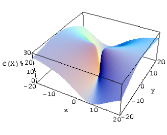
Figure 1: Example of optimized data-processing rule for the informationally complete POVM in Eq. (29). The plot shows the relative added noise in Eq. (27) for $X=\sigma_{z}+x\sigma_{x}+y\sigma_{y}$ versus $x$ and $y$

A quantitative estimate of $\epsilon(X)$ can be obtained from the following example in dimension two (see Fig. 1). Consider the POVM

$$\begin{split}P_{1}&=\begin{pmatrix}\frac{64}{1197}&-\frac{16}{1197}\\ -\frac{16}{1197}&\frac{40}{1197}\end{pmatrix},\ P_{2}=\begin{pmatrix}\frac{34}{1197}&\frac{2(1-16i)}{1197}\\ \frac{2(1+16i)}{1197}&\frac{34}{1197}\end{pmatrix},\\ P_{3}&=\begin{pmatrix}\frac{281}{399}&-\frac{18-32i}{1197}\\ -\frac{18+32i}{1197}&\frac{289}{399}\end{pmatrix},\ P_{4}=\begin{pmatrix}\frac{64}{399}&\frac{64(1-i)}{1197}\\ \frac{64(1+i)}{1197}&\frac{32}{399}\end{pmatrix},\\ &P_{5}=\begin{pmatrix}\frac{64}{1197}&\frac{-32(1+2i)}{1197}\\ -\frac{32(1-2i)}{1197}&\frac{160}{1197}\end{pmatrix}.\end{split}$$ (29)

The operator $X$ is the following selfadjoint operator

$$X=\begin{pmatrix}1&-2.24+i\\ -2.24-i&-1\end{pmatrix},$$ (30)

and for an ensemble of uniformly distributed pure states $\frac{1}{6}(\textrm{Tr}[X^{2}]+\textrm{Tr}[X]^{2})=\frac{1}{6}\textrm{Tr}[X^{2}]=2.34$. By direct calculation one obtains $\Sigma_{\Delta}=799.66$ and $\Psi=133.05$, and finally

$$\epsilon(X)\simeq 0.2,$$ (31)

which means a relative added noise of about $20\%$. This example shows that a correct processing can highly improve the statistics of expectation values, and eventually the convergence rate of tomographic state reconstruction. The additional error due to the use of the canonical dual instead of the optimal one is equivalent to a depolarizing channel with depolarization probability $0.09$.

In conclusion, we considered the general measurement scenario in which the ensemble average of an operator is determined via suitable data-processing of the outcomes of a quantum measurement described by a POVM. We have determined the optimal processing that minimizes the statistical error of the estimation. Contrarily to the widespread conviction, the optimal data-processing is generally not obtained via the canonical dual of the POVM, and the improvement due to optimization can be substantial. The present analysis has been carried out for finite spectrum and finite dimensions, however, it can be easily generalized to discrete spectrum in infinite dimensions for bounded operators and bounded duals, and, with more technicalities, even to continuous spectrum (the case of quantum homodyne tomography tomo ). We believe that the present result will allow to improve greatly many relevant experimental analysis of quantum measurements.

References

(1) J. Von Neumann, Mathematical Principles of Quantum
Mechanics, (Princeton University Press, Princeton, 1955).
(2) E. Arthurs and J. L. Kelly, Bell. Syst. Tech. J., 44 725-729 (1965).
(3) J. P. Gordon and W. H. Louisell, in Physics of Quantum Electronics, pp. 833-840,
McGraw-Hill, (New York, 1966).
(4) C. W. Helstrom Quantum Detection and Estimation
Theory,(Academic Press, New York, 1976).
(5) A. Chefles, Phys. Rev. A 64 062305 (2001).
(6) G. M. D’Ariano, P. Perinotti, and M. F. Sacchi, Europhys. Lett. 65, 165 (2004); J. Opt. B: Quantum Semiclass. Opt. 6, S487 (2004);
(7) G. M. D’Ariano, M. G. A. Paris, and M. F. Sacchi, Adv.
Imaging Electron Phys. 128, 205 (2003).
(8) F. Buscemi, G. M. D’Ariano, M. Keyl, P. Perinotti, and
R. F. Werner, J. Math. Phys. 46, 082109 (2005).
(9) G. M. D’Ariano, P. Lopresti, and L. Maccone, Phys.
Rev. Lett. 93, 250407 (2004).
(10) G. M. D’Ariano, J. Kahn, and M. F. Sacchi, Phys. Rev. A
72, 032310 (2005).
(11) R. J. Duffin and A. C. Schaeffer, Trans. Am. Math.
Soc. 72, 341 (1952); P. G. Casazza, Taiw. J. Math. 4,
129 (2000).
(12) P. Casazza, D. Han, and D. R. Larson, Contemp. Math.
247, 149 (1999).
(13) G. M. D’Ariano, P. Lopresti, and M. F. Sacchi, Phys.
Lett. A 272, 32 (2000).
(14) In infinite dimension generally one considers
as a Banach space (see Ref. banfram ) and the
condition is generally non trivial as in the finite
dimensional case.
(15) S. Li, Numer. Funct. Anal. Optim. 16, 1181 (1995).
(16) G. M. D’Ariano, P. Perinotti, and M. F.
Sacchi, Phys. Rev. A 72, 042108 (2005).
(17) R. B. Bhapat, Linear Algebra and Linear Models,
(Springer-Verlag, New York, 2000).
(18) Notice that since the swap operator acts on a
vector as , where
is the transpose of on the basis of Eq. (4),
by selfadjointness of one has , and
. Similarly , and then