Superposition of coherent states prepared in one mode of a dissipative bimodal cavity

Abstract

We solve the problem of the temporal evolution of one of two-modes embedded in a same dissipative environment and investigate the role of the losses after the preparation of a coherent state in only one of the two modes. Based on current cavity QED technology, we present a calculation of the fidelity of a superposition of coherent states engineered in a bimodal high-Q cavity. Our calculation demonstrates that the engineered superposition retains coherence for large times when the mean photon number of the prepared mode is on the order of unity.

Problems involving interaction of atoms and two modes of a electromagnetic field trapped into a high-Q cavity have increasingly received attention [1-14]. From the theoretical point of view, bimodal cavities were considered in a number of papers. For example, in [1] the phenomena of a degenerate and nondegenerate two-mode squeezing for a generalized Jaynnes-Cummings model with a two-level atom was considered; in [2] the authors show how to prepare W states, GHZ states, and two-qutrit entangled states using the multi-atom two-mode entanglement; in [3, 4, 5] schemes for teleporting entangled state of zero- and -one photon state from a bimodal cavity to another were proposed; in [6, 7]  the authors show how to build bilinear and quadratic Hamiltonians, thus opening the possibility to implement up- and down-conversion operations in two mode cavity QED. Recently, experiments with coherent control of atomic collision and controlled entanglement in bimodal cavities have been reported [8, 9], attracting even more attention to this topic.

It is to be noted that all the above mentioned papers do not take into account the effect of the environment, which plays an important role mainly when the decoherence time has to be considered. Damping of two modes of a cavity QED has been considered in Refs.[12, 13, 14], all of them using the Liouville approach. In [12] the behavior of  a two-level atom interacting with two modes of a light field in a cavity was investigated, and the effects of cavity damping were treated numerically for the special case of fields initially prepared in two mode squeezed vacuum state. In ref. [13] the authors studied the evolution of a two-level atom coupled to two modes of a dissipative cavity, and in ref. [14] the authors have investigated cross decay rates and robust (against dissipation) states in a system composed by two cavity modes in the presence of the same reservoir.

In this paper we review the problem of two modes in a lossy cavity QED. Our model differs from that of [13] since we take into account bosonic modes in a dissipative environment. Also, different from [12, 14], our model includes, beside two non-interacting bosonic modes subject to the same reservoir, a two-level atom interacting off-resonantly with one of the two modes of the bimodal cavity. Our Hamiltonian model is

$$H=H_{0}+H_{I}$$ (1)

where

$$H_{0}=\sum\limits_{j=1}^{2}\hbar\omega_{j}a_{j}^{\dagger}a_{j}+\sum\limits_{k}\hbar\omega_{k}b_{k}^{\dagger}b_{k}+\frac{\hbar\omega_{0}}{2}\sigma_{z}+\hbar a_{1}^{\dagger}a_{1}\chi_{1}\sigma_{z},$$ (2)

and

$$H_{I}=\sum\limits_{k}\sum\limits_{j=1}^{2}\hbar\left(\lambda_{jk}a_{j}^{\dagger}b_{k}+\lambda_{jk}^{\ast}a_{j}b_{k}^{\dagger}\right).$$ (3)

Here we consider a two-level atom composed by ground $\left|g\right\rangle$ and excited $\left|e\right\rangle$ state, $\ \sigma_{z}=\left|e\right\rangle\left\langle e\right|-\left|g\right\rangle\left\langle g\right|,$ $a_{j}^{\dagger}$ and $a_{j}$ are, respectively, the creation and annihilation operator for the j$th$ cavity mode of frequency $\omega_{j}$, whereas $b_{k}^{\dagger}$ and $b_{k}$ are the analogous operators for the k$th$ reservoir oscillator mode, whose corresponding frequency and coupling with the mode $j=1,2$ write $\omega_{k}$ and $\lambda_{jk}$, respectively. The atom-field coupling parameter is $\chi_{1}=\frac{g^{2}}{\delta_{1}}$, where $g$ is the Rabi frequency and $\delta_{1}=\left(\omega_{1}-\omega_{0}\right)$ is the detuning between the field frequency $\omega_{1}$ and the atomic frequency $\omega_{0}$. Note that the dispersive interaction occurs with only mode $1$. This is important for preparing superposition of coherent states [18]. Using the completeness relation for both atom and fields as given by coherent states, the Schrödinger state vector associated with Hamiltonian Eq.(1) can be written as

$$\left|\Phi(t)\right\rangle=\left|g\right\rangle\left|\phi_{g}(t)\right\rangle+\left|e\right\rangle\left|\phi_{e}(t)\right\rangle$$ (4)

where $\left|\phi_{\ell}(t)\right\rangle=\int\frac{d^{2}\alpha_{1}}{\pi}\int\frac{d^{2}\alpha_{2}}{\pi}\int\left\{\frac{d^{2}\beta_{k}}{\pi}\right\}\mathcal{A}_{\ell}\left|\alpha_{1},\alpha_{2},\left\{\beta_{k}\right\}\right\rangle$, $\ell=g,e$. The complex quantities $\alpha_{1},\alpha_{2},\left\{\beta_{k}\right\}$ stand for the eigenvalues of $a_{j}$ and $b_{k}$, respectively, and $\mathcal{A}_{\ell}\left(\alpha_{1},\alpha_{2},\left\{\beta_{k}\right\},t\right)$ are the expansion coefficients for $\left|\phi_{\ell}(t)\right\rangle$ in the basis of the coherent state products $\left|\alpha_{1},\alpha_{2},\left\{\beta_{k}\right\}\right\rangle$. The assumption of $\left|\left\{\beta_{k}\right\}\right\rangle$ for the reservoir follows from a remarkable property first proved by Mollow and Glauber [15], i.e., that at zero absolute temperature the reservoir receives coherently the excitation lost by a coherent state. The extension to finite temperature is considered in Ref.[16], where a phenomenological-operator approach to dissipation in cavity QED was proposed. Essentially, this extension consists in treating the reservoir plus the surrounding as a pure state provided that we include the degrees of freedom of whatever remain in the surrounding, in such way that we obtain a mixed (thermal) state after tracing out the degrees of freedom of whatever was included. Because the orthogonality of the atomic states and Eq.(1-4), we can obtain the uncoupled time-dependent Schröedinger equations

$$i\hslash\frac{d}{dt}\left|\phi_{\ell}(t)\right\rangle=H_{\ell}\left|\phi_{\ell}(t)\right\rangle,$$ (5)

where $H_{\ell}=H_{\ell 0}+H_{I}$, and

$$H_{\ell 0}=\hbar\left(\omega_{1}\pm\chi\right)a_{1}^{\dagger}a_{1}+\hbar\omega_{2}a_{2}^{\dagger}a_{2}+\sum\limits_{k}\hbar\omega_{k}b_{k}^{\dagger}b_{k}.$$ (6)

Note that the problem has been reduced to that of dissipation of two modes of the cavity field whose frequency $\omega_{1}$ of mode $1$ has been shifted by $-\chi$ ($\chi$) when interacting with the ground (excited) state of the atom. To solve the problem of  the evolution of an arbitrary initial state prepared in one of the two modes we pursue a different approach from that of Refs. [12, 13, 14]. Instead of following the evolution of the two modes at once, we will follow rightly to the mode of interest, assumed as mode $1$. A convenient way to perform this can be done by the method of the reduced density operator [17]. For this purpose we first calculate the characteristic function $G$ in the normal order, then the Glauber-Sudarshan $P$ representation, and finally the reduced density operator $\rho_{1}(t)$ for mode $1$. The $G$ function for mode $1$ in the Heisenberg picture reads

$$G(\eta,\eta^{\ast},t)=Tr_{2R}\left\{\rho_{12R}(0)\exp\left[\eta a_{1}^{\dagger}(t)\right]\exp\left[-\eta^{\ast}a_{1}(t)\right]\right\},~{}~{}~{}~{}$$ (7)

where $\rho_{12R}(0)$ is the density operator for the whole system composed by modes $1$,$2$ and the reservoir at the instant $t=0$, and $Tr_{2R}$ indicates the trace on mode 2 and reservoir. The Glauber-Sudarshan $P$ representation is given by the two-dimensional Fourier transform of the characteristic function $G$:

$$P\left(\xi,\xi^{\ast},t\right)=\int G(\eta,\eta^{\ast},t)\exp\left(-\eta\xi^{\ast}+\eta^{\ast}\xi\right)\frac{d^{2}\eta}{\pi^{2}},$$ (8)

while the reduced density operator for mode $1$ of the cavity field state is given by the diagonal representation of $P\left(\xi,\xi^{\ast},t\right)$:

$$\rho_{1}(t)=\int P\left(\xi,\xi^{\ast},t\right)\left|\xi\right\rangle\left\langle\xi\right|d^{2}\xi.$$ (9)

To apply this method, we will need to solve the following Heisenberg equations for modes $a_{j}$ corresponding to the Hamiltonian Eq.(6) in order to substitute them in Eq.(7):

$$\dot{a_{j}} = -i\omega_{j\ell}a_{j}-i\sum\limits_{k}\lambda_{ik}^{\ast}b_{k}$$ (10)

$$\dot{b_{k}} = -i\omega_{k}b_{i}-i\sum\limits_{i=1}^{2}\lambda_{ik}a_{i},$$ (11)

where $\omega_{j\ell}=\left(\omega_{1}\pm\chi\right)$ if $j=1$ and the minus (plus) signal depends on the initial state $g$ ($e$) of the atom, or $\omega_{j\ell}=\omega_{2}$ if $j=2$. Eqs.(10-11) can be solved, for example, by Laplace transform. In doing so, we multiply both sides of Eqs.(10-11) by $\exp(-st),$ integrate from $0$ to $\infty$ and evaluate the inverse Laplace transform under the Wigner-Weisskopf approximation [17]

$$\sum_{k}\frac{\lambda_{kj}^{\ast}\lambda_{kj^{\prime}}}{s+i\omega_{k}}\rightarrow i\Delta\omega_{jj^{\prime}}+\frac{\gamma_{jj^{\prime}}}{2};~{}~{}~{}~{}~{}~{}j,~{}j^{\prime}=1,2$$

where $\Delta\omega_{jj}$, $\gamma_{jj}$ denote the shift in the energy and the decay rate of the $j$-mode, respectively, and $\Delta\omega_{jj^{\prime}},$ $\gamma_{jj^{\prime}}$ ($j\neq j^{\prime}$) the corresponding cross shift in the energy and the cross decay rates [14] for modes $1$,$2$. The results for modes $1$ and $2$ are

$$a_{1}(t) = u_{11}(t)a_{1}(0)+u_{12}(t)a_{2}(0)+\sum\limits_{k}\vartheta_{1k}(t)b_{k}(0),~{}~{}~{}~{}~{}~{}~{}$$ (12)

$$a_{2}(t) = u_{22}(t)a_{2}(0)+u_{21}(t)a_{1}(0)+\sum\limits_{k}\vartheta_{2k}(t)b_{k}(0),~{}~{}~{}~{}~{}~{}~{}$$ (13)

where

$$u_{11}(t) = \exp\left[-\frac{(A+B)}{2}t\right]\left[\frac{\left(B-A\right)}{\sqrt{\left(B-A\right)^{2}+4\left|C\right|^{2}}}\sinh\left(\sqrt{\frac{\left(B-A\right)^{2}+4\left|C\right|^{2}}{2}}t\right)\right.$$

$$+ \left.\cosh\left(\sqrt{\frac{\left(B-A\right)^{2}+4\left|C\right|^{2}}{2}}t\right)\right]$$

$$u_{12}(t) = -\exp\left[-\frac{(A+B)}{2}t\right]\left[\frac{2C}{\sqrt{\left(B-A\right)^{2}+4\left|C\right|^{2}}}\sinh\left(\sqrt{\frac{\left(B-A\right)^{2}+4\left|C\right|^{2}}{2}}t\right)\right],$$

and

$$\vartheta_{1k}(t) = i(\lambda_{k2}^{\ast}C-\lambda_{k1}^{\ast}-\lambda_{k1}^{\ast}B)$$ (16)

$$\times \left\{\frac{\exp\left[-\left(\frac{A+B-\sqrt{(B-A)^{2}+4\left|C\right|^{2})}}{2}\right)t\right]}{(\frac{-(B+A)+\sqrt{(B-A)^{2}+4\left|C\right|^{2}}}{2}+i\omega_{k})\sqrt{(B-A)^{2}+4\left|C\right|^{2}}}\right.$$

$$+ \frac{\exp\left[-(\frac{A+B+\sqrt{(B-A)^{2}+4\left|C\right|^{2})}}{2})t\right]}{(\frac{(B+A)+\sqrt{(B-A)^{2}+4\left|C\right|^{2}}}{2}-i\omega_{k})\sqrt{(B-A)^{2}+4\left|C\right|^{2}}}$$

$$- \left.\frac{\exp(-i\omega t)}{(\frac{(B+A)+\sqrt{(B-A)^{2}+4\left|C\right|^{2}}}{2}-i\omega_{k})(\frac{-(B+A)+\sqrt{(B-A)^{2}+4\left|C\right|^{2}}}{2}+i\omega_{k})}\right\}$$

with

$$A = i\left(\omega_{1}\pm\chi+\Delta\omega_{1}\right)+\gamma_{11}/2$$ (17)

$$B = i\left(\omega_{2}\pm\chi+\Delta\omega_{2}\right)+\gamma_{12}/2$$ (18)

$$C = -i\Delta\omega_{12}-\gamma_{12}/2.$$ (19)

Functions$\ u_{21}(t)$, $u_{22}(t)$ and $\vartheta_{2k}(t)$ can be obtained from $u_{12}(t)$, $u_{11}(t)$ and $\vartheta_{1k}(t)$, respectively, simply replacing $C$ by $C^{\ast}$, $A$ by $B$, $1$ by $2$ and vice-versa.

It is now straightforward to obtain $\rho_{1}(t)$ for an arbitrary initial state if we note that any initial state $\sum_{n,m}C_{nm}\left|m\right\rangle_{1}\left|n\right\rangle_{2}$ can be 1written in its most general form as

$$\rho_{12R}(0) = \sum\limits_{n,m,j,k}\int d^{2}\alpha_{1}d^{2}\alpha_{2}d^{2}\beta_{1}d^{2}\beta_{2}C_{nmjk}\left|\alpha_{1}\right\rangle_{11}\left\langle\alpha_{2}\right|\left|\beta_{1}\right\rangle_{22}\left\langle\beta_{2}\right|$$ (20)

$$\times \int\left\{d^{2}\gamma_{k}\right\}P\left(\left\{\gamma_{k}\right\}\right)\left|\left\{\gamma_{k}\right\}\right\rangle_{R}\left\langle\left\{\gamma_{k}\right\}\right|$$

where modes $1$ and $2$ were expanded in coherent states and the reservoir is in a thermal state $\sum\limits_{k}p_{k}\left|n_{k}\right\rangle_{R}\left\langle n_{k}\right|$ characterized by an average photon number in the k$th$ mode $\left\langle n_{k}\right\rangle=1/\left[\exp(\hslash\omega_{k}/kT-1)\right]$ according to $p_{k}=\frac{\left\langle n_{k}\right\rangle^{n}}{\left(1+n_{k}\right)^{n+1}}$, and was expanded in the diagonal representation with $P\left(\left\{\gamma_{k}\right\}\right)=$ $\prod\limits_{k}\frac{1}{\pi\left\langle n_{k}\right\rangle}\exp\left(-\frac{\left|\gamma_{k}\right|^{2}}{\left\langle n_{k}\right\rangle}\right)$. The characteristic function for mode $1$ corresponding to the initial state of Eq.(20) reads

$$G(\eta,\eta^{\ast},t) = \sum\limits_{n,m,j,k}\int d^{2}\alpha_{1}d^{2}\alpha_{2}d^{2}\beta_{1}d^{2}\beta_{2}C_{nmjk~{}~{}2}\left\langle\beta_{2}\right|\left.\beta_{1}\right\rangle_{21}\left\langle\alpha_{2}\right|\left.\alpha_{1}\right\rangle_{1}$$ (21)

$$\times \exp\left[-\eta^{\ast}u_{11}(t)\alpha_{01}+\eta u_{11}^{\ast}(t)\alpha_{02}^{\ast}\right]\exp\left[-\eta^{\ast}u_{12}(t)\beta_{01}+\eta u_{12}^{\ast}(t)\beta_{02}^{\ast}\right]$$

$$\times \prod\limits_{k}\exp\left[-\left|\eta\right|^{2}\left|\vartheta_{1k}(t)\right|^{2}\left\langle n_{k}\right\rangle\right],$$

where we have written $f(0)=f_{0}$. The Glauber-Sudarshan $P\left(\xi,\xi^{\ast},t\right)$ representation for mode $1$ as given by Eq.(8) is the Fourier transform of Eq.(21):

$$P\left(\xi,\xi^{\ast},t\right) = \sum\limits_{n,m,j,k}\int d^{2}\alpha_{1}d^{2}\alpha_{2}d^{2}\beta_{1}d^{2}\beta_{2}C_{nmjk}(\beta\alpha)\frac{{}_{1}\left\langle\alpha_{2}\right|\left.\alpha_{1}\right\rangle_{12}\left\langle\beta_{2}\right|\left.\beta_{1}\right\rangle_{2}}{\pi D(t)}$$ (22)

$$\times \exp\left(-\frac{\left[\xi-u_{11}(t)\alpha_{01}-u_{12}(t)\beta_{10}\right]\left[\xi^{\ast}-u_{11}^{\ast}(t)\alpha_{02}^{\ast}-u_{12}^{\ast}(t)\beta_{20}^{\ast}\right]}{D(t)}\right)$$

where $D(t)=\sum\left|\vartheta_{1k}(t)\right|^{2}\left\langle n_{k}\right\rangle$. The reduced density operator for mode $1$ can now be obtained using Eq.(9).

In the following, let us consider the important case of engineering two coherent states inside a single bimodal high$-Q$ cavity with one of the two modes supporting a coherent state and the other mode being prepared in a superposition of coherent state (SCS) in the presence of a reservoir cooled to $0$ K, i.e., when the initial state is given by

$$\mathcal{N}_{p}\left(\left|\alpha(0)\right\rangle_{1}+\left|-\alpha(0)\right\rangle_{1}\right)\left|\alpha(0)\right\rangle_{2}\left|\left\{0\right\}\right\rangle_{R}.$$ (23)

This example is the analogous of the “Schrödinger cat state” studied in Ref.[18] in the context of unimodal cavity QED, in the microwave domain, to unravel the role of the environment in the transition from the quantum to classical dynamics. For calculating the corresponding evolution of the SCS of Eq.(23), it is enough to consider the evolution of the initial state $\rho_{12R}(0)$ as given by Eq.(20), and left $\alpha_{1}$, $\alpha_{2}$ and $\beta_{1},$ $\beta_{2}$ assuming the values $\pm\alpha$ to compose the complete density operator. Using Eqs.(21-22) and taking the limit $D(t)\rightarrow 0$ for zero temperature, we obtain for the evolved mode $1$ in Eq.(20)

$$\rho_{1}(t) = \frac{{}_{2}\left\langle\beta_{20}\right|\left.\beta_{10}\right\rangle_{2}~{}~{}_{1}\left\langle\alpha_{20}\right|\left.\alpha_{10}\right\rangle_{1}}{{}_{1}\left\langle-u_{11}(t)\alpha_{20}+u_{21}(t)\beta_{01}\right|\left.u_{11}(t)\alpha_{10}+u_{12}(t)\beta_{02}\right\rangle_{1}}$$ (24)

$$\times \left|u_{11}(t)\alpha_{10}+u_{12}(t)\beta_{01}\right\rangle_{11}\left\langle-u_{11}(t)\alpha_{20}+u_{12}(t)\beta_{02}\right|.$$

Now, taking into account Eq.(24), when considering the initial state as given by Eq.(23), $\rho_{1}(t)$ reads

$$\rho_{1}(t) = \mathcal{N}_{e}\left\{\left|\left[u_{11}(t)+u_{12}(t)\right]\alpha_{10}\right\rangle_{1}\left\langle\left[u_{11}(t)+u_{12}(t)\right]\alpha_{10}\right|\right.$$ (25)

$$+ \left.\left|\left[-u_{11}(t)+u_{12}(t)\right]\alpha_{10}\right\rangle_{1}\left\langle\left[-u_{11}(t)+u_{12}(t)\right]\alpha_{10}\right|\right.$$

$$+ \left.Z(t)\left[\left|\left[u_{11}(t)+u_{12}(t)\right]\alpha_{10}\right\rangle_{1}\left\langle\left[-u_{11}(t)+u_{12}(t)\right]\alpha_{10}\right|+h.c.\right]\right\}$$

where $h.c.$ means Hermitian conjugate and

$$Z(t) = \exp\left\{-2\left|\alpha_{0}\right|^{2}\left[1-\left|u_{11}(t)\right|^{2}\right.-\left.\frac{u_{12}(t)u_{11}^{\ast}(t)}{2}+\frac{u_{12}^{\ast}(t)u_{11}(t)}{2}\right]\right\}$$ (26)

is the term responsible by decoherence. To evaluate the errors in the SCS prepared in one of the two modes caused by the environment and due to the presence of the coherent state in the other mode, we calculate the fidelity $\digamma=_{1}\left\langle\Psi\right|\rho_{1}(t)\left|\Psi\right\rangle_{1}$, where $\rho_{1}(t)$ and $\left|\Psi\right\rangle_{1}$ is the evolved (mixed) and the prepared (ideal) SCS, respectively, for the prepared SCS in mode $1$. After a straightforward calculation and rearranging the terms, we obtain

$$\digamma = \mathcal{N}_{p}^{2}\mathcal{N}_{e}^{2}e^{-\left(\left|\alpha(t)\right|^{2}+\left|\alpha_{0}\right|^{2}\right)}\left\{\cosh\left[\alpha_{0}^{\ast}\alpha(t)+\alpha_{0}\alpha^{\ast}(t)\right]\right.$$ (27)

$$+ \left.\cosh\left[\alpha_{0}^{\ast}\alpha(t)-\alpha_{0}\alpha^{\ast}(t)\right]\right\}[2+Z(t)+Z^{\ast}(t)],$$

where the normalization factors are $\mathcal{N}_{p}=[1+e^{-2\left|\alpha_{0}\right|^{2}}]^{-\frac{1}{2}}$, $\mathcal{N}_{e}=[2+(Z(t)e^{-2\left|\alpha(t)\right|^{2}}+hc)]^{-\frac{1}{2}}$ for the prepared (ideal) and the evolved (mixed) states, respectively, and $\alpha(t)=\alpha_{0}\left[u_{11}(t)+u_{12}(t)\right]$.

Fig.1 shows the fidelity of the prepared SCS state considering parameters recently used in experiments with two modes of a cavity QED [8]. As usual, we have disregarded the cavity-field losses during the considerably short time during which the atom crosses the cavity, about $10^{-4}s$. As expected, as the field excitation increases, the fidelity decays faster. For $\alpha$ around unity, the fidelity indicates a large time, as compared with the damping time, during which the SCS remains available for further operations.

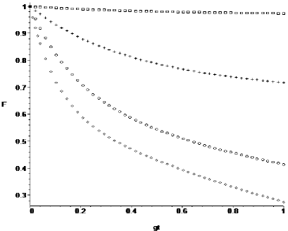
Figure 1: Fidelity for the prepared SCS for $\alpha=0.5$ (box), $1.0$ (cross), $1.5$ (circle), and $2.0$ (diamond). Here we used the experimental values $T_{1}=$ $1$ $ms$ and $T_{2}=0.9$ $ms$ for the damping time corresponding to mode$-1$ and mode$-2$, respectively.

In conclusion, in this paper we presented, for the first time, a calculation of the fidelity for a superposition of coherent states prepared in one of two modes of a cavity QED. To achieve this goal, we solved the problem of two modes embedded in a same dissipative environment. Different from previous studies, our problem includes off-resonantly interaction between a two-level atom, necessary for preparing the coherent state superposition, and one of the two modes. Our result indicated high-fidelity of the prepared superposition of coherent states when its mean photon number is on order of unity.

We thank the VPG/Vice-Reitoria de Pós-Graduação e Pesquisa-UCG (NGA), CAPES(IPQ, WBC), and CNPq (NGA), Brazilian Financial Agencies, for the partial support.

References

References

• [1] A. M. Abdel-Hafez, Phys. Rev. A 45, 6610 (1992).
• [2] Asoka Biswas, G. S. Agarwal, J. Mod. Opt. 51, 1627 (2004).
• [3] G. Pires, N. G. de Almeida, A. T. Avelar, and B. Baseia, Phys. Rev. A 70, 025803 (2004);
• [4] Wesley B. Cardoso, A. T. Avelar, B. Baseia, and N. G. de Almeida, Phys. Rev. A 72, 045802 (2005).
• [5] Zhen-Biao Yang, J. Phys. B: At. Mol. Opt. Phys. 39 603 (2006).
• [6] F. O. Prado, N. G. de Almeida, M. H. Y. Moussa, and C. J. Villas-Bôas, Phys. Rev. A 73, 043803 (2006).
• [7] R. M. Serra, C. J. Villas-Bôas, N. G. de Almeida, and M. H. Y. Moussa, Phys. Rev. A 71, 045802 (2005).
• [8] A. Rauschenbeutel, P. Bertet, S. Osnaghi, G. Nogues, M. Brune, J. M. Raimond, and S. Haroche, Phys. Rev. A 64, 050301 (2001).
• [9] S. Osnaghi, P. Bertet, A. Auffeves, P. Maioli, M. Brune, J. M. Raimond, and S. Haroche, Phys. Rev. Lett. 87, 037902 (2001).
• [10] A. R. Bosco de Magalhaes, S. G. Mokarzel, M. C. Nemes, M. O. Terra Cunha, Physica A 341, 234 (2004).
• [11] Ke-Hui Song, Chinese Physics, 15 286 (2006).
• [12] Shih-Chuan Gou, Phys. Rev. A 40, 5116 (1989).
• [13] A. Napoli, Xiang-Ming Hu, A. Messina, Phys Lett A, 308, 329 ((2003).
• [14] R. Rossi Jr., A. R. Bosco de Magalhães, and M. C. Nemes, Physica A 365, 402 (2006); quant-ph/0410200.
• [15] B. R. Mollow and R. J. Glauber, Phys. Rev. 160, 1076 (1967).
• [16] N. G. de Almeida, R. Napolitano, and M. H. Y. Moussa, Phys. Rev. A 62, 033815 (2000).
• [17] L. Mandel and E.Wolf, Optical Coherence and Quantum Optics (Cambridge Univ. Press,1995); M. O. Scully, and M. S. Zubairy, Quantum Optics (Cambridge Univ. Press, 1997).
• [18] M. Brune, E. Hagley, J. Dreyer, X. Maître, A. Maali, C. Wunderlich, J. M. Raimond, and S. Haroche, Phys. Rev. Lett. 77, 4887 (1996).