Passage-time distributions from a spin-boson detector model

Abstract

The passage-time distribution for a spread-out quantum particle to traverse a specific region is calculated using a detailed quantum model for the detector involved. That model, developed and investigated in earlier works, is based on the detected particle’s enhancement of the coupling between a collection of spins (in a metastable state) and their environment. We treat the continuum limit of the model, under the assumption of the Markov property, and calculate the particle state immediately after the first detection. An explicit example with 15 boson modes shows excellent agreement between the discrete model and the continuum limit. Analytical expressions for the passage-time distribution as well as numerical examples are presented. The precision of the measurement scheme is estimated and its optimization discussed. For slow particles, the precision goes like $E^{-3/4}$, which improves previous $E^{-1}$ estimates, obtained with a quantum clock model.

I Introduction

Time-of-flight measurements are a standard tool for many experimentalists. Since the particles or atoms involved are usually fast, their center-of-mass motion is typically treated classically, yielding a simple description of the time-of-flight measurement. But as the diffraction and interference experiments using temporal (instead of spatial) slits of Szriftgiser et. al have shown Szriftgiser et al. (1996), such a description of the center-of-mass motion by means of classical physics is not always sufficient: the advance of cooling techniques has made it possible to create ultracold gases in a trap and produce very slow atoms, e.g., by opening the trap. Whenever such ultracold atoms are involved, the spatial extent and the spreading of the wave function can show noticeable effects. Even the seemingly simple question of the time spent by a particle in a given region of space does not possess a simple and definite answer. Related to this “dwell-time” problem are the problems of “passage time,” concentrating on those particles that actually cross the region of interest and are not reflected, and “tunneling time” in the case of a barrier that classically cannot be traversed inside the region of interest. These problems have on one hand been treated axiomatically aiming at ideal quantities relying only on the system of interest, see, e.g., Refs. Smith (1960); Sokolovski and Baskin (1987); Jaworski and Wardlaw (1988); Muga et al. (1992). Other approaches may be called “operational” in the sense that a sort of “measurement device” is introduced to which the system of interest is coupled; see, e.g., Refs. Baz’ (1967); Rybachenko (1967); Balcou and Dutriaux (1997); Salecker and Wigner (1958); Peres (1980); Alonso et al. (2003). For a critical review on different approaches to tunneling times see, e.g., Refs. Hauge and Støvneng (1989); Landauer and Martin (1994).

A distinction that can be drawn between the various time-related quantities recalled above concerns whether they are pre- or post- decoherence. Since the present work models the measurement apparatus, it can be thought of as post-decoherence; in fact it is one of our objectives to include decoherence-inducing processes, thereby eliminating some of the black magic of quantum measurement. On the other hand, one can take, for example, a path integral approach to tunneling time Schulman and Ziolkowski (1989); Sokolovski and Baskin (1987) in which the paths are sorted by (variously defined) times spent in the barrier region. For these paths, amplitudes are retained, so it is very much a pre-decoherence calculation. As a result interpretive issues arise (discussed for example by Yamada (1999)) which do not enter in the present work.

In the present paper we investigate a particular measurement scheme for passage times, mimicking the way a time-of-flight experiment is typically performed: Employing a particular spin-boson detector model for measuring quantum arrival times investigated in Ref. Hegerfeldt et al. (2006), our measurement scheme involves two measurements of arrival time by means of this detector, one upon entering the region of interest and one when exiting; see Fig. 1.

Figure 1: The first detector detects the particle at entry into the region of interest, the second one at exit. From the correlation of these two arrival-time distributions, the passage-time distribution is obtained. The $x$-positions correspond to the numerical examples discussed in Section IV.2.

This scheme can be expected to distort the particle’s wave function less than a scheme based on the (semi-)continuous coupling of the particle to a measurement device. Indeed, it will be seen that a passage-time measurement by means of “slow” detectors yields a rather broad passage-time distribution. But detectors responding quickly to the presence of the particle also yield a broad distribution. This will be shown to be a quantum effect involving the Heisenberg uncertainty relation. However, there is an intermediate range for the detector parameters yielding optimal results. In the best case the precision of the measurement can be estimated to behave like $E^{-3/4}$, improving the results obtained from clock models Peres (1980); Alonso et al. (2003).

In Sec. II we review the detector model and its application to quantum arrival-times. In Sec. III the particle’s wave function immediately after the detection is investigated, and in Sec. IV analytical formulas for the application of the detector model to passage times are derived. Numerical examples are investigated in Sec. IV.2. For simplicity, we concentrate there on passage times for free particles; the extension to passage times in the presence of barriers, and thus to tunneling times, should proceed on similar lines. The precision of the measurement scheme is estimated in Sec. V.

II The detector model and its arrival-time distribution

We briefly review the detector model introduced in Refs. Gaveau and Schulman (1990); Schulman (1991, 1997) and the arrival-time distribution obtained from this model in Ref. Hegerfeldt et al. (2006). The detector consists of a three-dimensional array of spins with ferromagnetic interaction in a metastable state. The spins are weakly coupled to the environment, modeled as a bath of bosons. The effect of the particle to be observed is to strongly enhance the spin-bath coupling when the particle’s wave function overlaps with that of a spin. Thus when the particle is close to a spin, this spin flips with strongly increased probability due to the enhanced spin-bath coupling. By means of the ferromagnetic interaction, this in turn triggers the subsequent spontaneous flipping of the neighboring spins, and finally, by a domino effect, of all spins, even in the absence of the particle. In this way, the single spin flip induced by the presence of the particle is amplified to a macroscopic event, and either the change in the detector state or in the bath state can be measured.

The Hamiltonian for this model is

$$H=H_{\mathrm{part}}+H_{\mathrm{det}}+H_{\mathrm{bath}}+H_{\mathrm{spon}}+H_{\mathrm{coup}}\,,$$ (1)

where we use the following definitions:

$$H_{\mathrm{part}}=\frac{\hat{\mathbf{p}}^{2}}{2m}\,$$ (2)

is the free Hamiltonian of the particle;

$$H_{\mathrm{det}}=\sum_{j}\frac{\hbar\omega_{0}^{(j)}}{2}\hat{\sigma}_{z}^{(j)}-\sum_{j<k}\frac{\hbar\omega_{J}^{(jk)}}{2}\hat{\sigma}_{z}^{(j)}\otimes\hat{\sigma}_{z}^{(k)}$$ (3)

with $\left|\uparrow\right\rangle_{j}$ denoting the excited state of the $j^{\mathrm{th}}$ spin and

$$\hat{\sigma}_{z}^{(j)}\equiv\left|\uparrow\right\rangle_{j\;j}\!\left\langle\uparrow\right|\,-\,\left|\downarrow\right\rangle_{j\;j}\!\left\langle\downarrow\right|\,,$$ (4)

is the free Hamiltonian of the detector; $\hbar\omega_{0}^{(j)}$ is the energy difference between ground state and excited state of the $j^{\mathrm{th}}$ spin, and $\hbar\omega_{J}^{(jk)}\geq 0$ is the coupling energy between the spins $j$ and $k$. Further,

$$H_{\mathrm{bath}}=\sum_{\boldsymbol{\ell}}\hbar\omega_{\boldsymbol{\ell}}\hat{a}_{\boldsymbol{\ell}}^{\dagger}\hat{a}_{\boldsymbol{\ell}},$$ (5)

where $\hat{a}_{\boldsymbol{\ell}}$ is the annihilation operator for a boson with wave vector $\boldsymbol{\ell}$, is the free Hamiltonian of the environment, modeled as a bath of bosons, and

$$H_{\mathrm{spon}}=\sum_{j,\boldsymbol{\ell}}\hbar\left(\gamma_{\boldsymbol{\ell}}^{(j)}e^{if_{\boldsymbol{\ell}}^{(j)}}\hat{a}_{\boldsymbol{\ell}}^{\dagger}\hat{\sigma}_{-}^{(j)}+\mathrm{h.c.}\right)$$ (6)

with

$$\hat{\sigma}_{-}^{(j)}\equiv\left|\downarrow\right\rangle_{j\;j}\!\left\langle\uparrow\right|,\;\hat{\sigma}_{+}^{(j)}\equiv\left(\hat{\sigma}_{-}^{(j)}\right)^{\dagger}=\left|\uparrow\right\rangle_{j\;j}\!\left\langle\downarrow\right|,$$ (7)

and the coupling constants $\gamma_{\boldsymbol{\ell}}^{(j)}$ and the phases $f_{\boldsymbol{\ell}}^{(j)}$ depending on the particular realization of the detector and the bath, describes the permanent spin-bath coupling. The spin-bath coupling is strongly enhanced in the particle’s presence due to

$$H_{\mathrm{coup}}^{(j)}=\sum_{j}\chi^{(j)}\left(\hat{\mathbf{x}}\right)\sum_{\boldsymbol{\ell}}\hbar\left(g_{\boldsymbol{\ell}}^{(j)}e^{if_{\boldsymbol{\ell}}^{(j)}}\hat{a}_{\boldsymbol{\ell}}^{\dagger}\hat{\sigma}_{-}^{(j)}+\mathrm{h.c.}\right),$$ (8)

with

$$\left|g_{\boldsymbol{\ell}}^{(j)}\right|^{2}\gg\left|\gamma_{\boldsymbol{\ell}}^{(j)}\right|^{2};$$ (9)

thus, the enhanced coupling of the $j^{\mathrm{th}}$ spin to the bath is proportional to a sensitivity function $\chi^{(j)}(\mathbf{x})$ which vanishes outside the region ${\mathcal{G}}^{(j)}$ where the $j^{\mathrm{th}}$ spin is located. An example would be the characteristic function which is $1$ on ${\mathcal{G}}^{(j)}$ and zero outside. It will be assumed in the sequel that the Markov property [see Eq. (16)] holds in an appropriate continuum limit. Initially, the system is prepared in the state

$$\left|\Psi_{0}\right\rangle=\left|0\right\rangle\left|\uparrow_{1}\ldots\uparrow_{D}\right\rangle\left|\psi_{0}\right\rangle,$$ (10)

where $\left|0\right\rangle$ is the ground state of the bath (no bosons present), and $\left|\psi_{0}\right\rangle$ denotes the spatial wave function of the particle. For the $\hbar\omega_{0}^{(j)}$ only slightly above the energetic threshold set by the ferromagnetic spin-spin coupling, and $\gamma_{\boldsymbol{\ell}}^{(j)}$ sufficiently small, the probability of a spontaneous spin flip (false positive) is very small Gaveau and Schulman (1990); Schulman (1991, 1997). But when the particle is close to the $j^{\mathrm{th}}$ spin, the excited state $\left|\uparrow\right\rangle_{j}$ decays much more quickly, due to the enhanced coupling, “$g_{\boldsymbol{\ell}}^{(j)}$,” of the spin to the bath. Then, the ferromagnetic force experienced by its neighbors is strongly reduced, and these spins can therefore flip rather quickly, even in the absence of the particle, by means of the $\gamma_{\boldsymbol{\ell}}^{(j)}$. The first spin flip will be amplified to a macroscopic event by the previously mentioned domino effect Gaveau and Schulman (1990); Schulman (1991, 1997).

In Ref. Hegerfeldt et al. (2006) we investigated, by means of the quantum jump approach qu_ , the application of this detector model to arrival-time measurements. The bath modes were indexed by wave vectors

$$\boldsymbol{\ell}=\frac{2\pi}{L_{\mathrm{bath}}}\left(\begin{array}[]{c}n_{1}\\ n_{2}\\ n_{3}\end{array}\right),\;\;n_{i}\in\mathbb{N}_{0},$$ (11)

and the coupling constants were assumed to be of the form

$$g_{\boldsymbol{\ell}}^{(j)} = \left(\Gamma^{(j)}(\omega_{\ell},\mathbf{e}_{\boldsymbol{\ell}})+{\mathcal{O}}(L_{\mathrm{bath}}^{-1})\right)\sqrt{\frac{\omega_{\ell}}{L_{\mathrm{bath}}^{3}}},$$

$$\gamma_{\boldsymbol{\ell}}^{(j)} = \left(\Gamma_{\mathrm{spon}}^{(j)}(\omega_{\ell},\mathbf{e}_{\boldsymbol{\ell}})+{\mathcal{O}}(L_{\mathrm{bath}}^{-1})\right)\sqrt{\frac{\omega_{\ell}}{L_{\mathrm{bath}}^{3}}}$$ (12)

with $\omega_{\ell}=c(\omega_{\ell})\ell$, $\mathbf{e}_{\boldsymbol{\ell}}=\boldsymbol{\ell}/\ell$, and

$$\left|\Gamma^{(j)}(\omega_{\ell},\mathbf{e}_{\boldsymbol{\ell}})\right|^{2}\gg\left|\Gamma_{\mathrm{spon}}^{(j)}(\omega_{\ell},\mathbf{e}_{\boldsymbol{\ell}})\right|^{2}.$$ (13)

We introduce “modified resonance frequencies”

$$\tilde{\omega}_{0}^{(j)}\equiv\omega_{0}^{(j)}-\sum_{{k=1}\atop{k\neq j}}^{D}\omega_{J}^{(jk)},$$ (14)

which incorporate the ferromagnetic spin-spin coupling. The correlation function $\kappa_{\overline{g}g}^{(j)}(\tau)$ is defined by

$$\kappa_{\overline{g}g}^{(j)}(\tau)\equiv\sum_{\boldsymbol{\ell}}\left|g_{\boldsymbol{\ell}}^{(j)}\right|^{2}e^{-i(\omega_{\ell}-\widetilde{\omega}_{0}^{(j)})\tau},$$ (15)

and similarly for $\kappa_{\overline{g}\gamma}^{(j)}$, $\kappa_{\overline{\gamma}g}^{(j)}$, and $\kappa_{\overline{\gamma}\gamma}^{(j)}$. It is assumed that in the continuum limit, $L_{\mathrm{bath}}\rightarrow\infty$, the correlation functions satisfy the Markov property, i.e.,

$$\kappa_{\overline{g}g}^{(j)}(\tau)\approx 0\quad\mathrm{if}\quad\tau>\tau_{\mathrm{c}},$$ (16)

for some small correlation time $\tau_{\mathrm{c}}$, and likewise for the other correlation functions. This is the case, e.g., if $\Gamma(\omega_{\ell},\mathbf{e}_{\boldsymbol{\ell}})$ is independent of $\omega_{\ell}$, as in quantum optics.

Let $\left|\psi_{\mathrm{cond}}^{t}\right\rangle$ denote the time evolution of the spatial wave function under the condition that no boson is detected at least until time $t$ (“conditional time evolution”). Then

$$P_{0}(t)\equiv\left\langle\psi_{\mathrm{cond}}^{t}\right|\left.\!\psi_{\mathrm{cond}}^{t}\right\rangle$$ (17)

is the probability that no detection occurred until $t$, which is decreasing in time, and

$$w_{1}(t)\equiv-\frac{dP_{0}}{dt}(t)$$ (18)

is the probability density for the first detection to occur at time $t$. In Ref. Hegerfeldt et al. (2006) it was shown that $\left|\psi_{\mathrm{cond}}^{t}\right\rangle$ obeys a “conditional Schrödinger equation” of the form

$$i\hbar\frac{\partial}{\partial t}\left|\psi_{\mathrm{cond}}^{t}\right\rangle=H_{\mathrm{cond}}\left|\psi_{\mathrm{cond}}^{t}\right\rangle$$ (19)

with a Hamiltonian containing a complex potential,

$$H_{\mathrm{cond}}=\frac{\hat{\mathbf{p}}^{2}}{2m}+\frac{\hbar}{2}\left[\delta_{\mathrm{shift}}(\hat{\mathbf{x}})-iA(\hat{\mathbf{x}})\right]\,,$$ (20)

where $\delta_{\mathrm{shift}}(\hat{\mathbf{x}})$ and $A(\mathbf{x})$ are defined as follows. $A(\mathbf{x})$ is a position-dependent detector decay rate,

$$A\left(\mathbf{x}\right) = 2\,\mathrm{Re}\,\sum_{j}\int_{0}^{\infty}d\tau\,\{\kappa_{\overline{g}g}^{(j)}(\tau)\chi^{(j)}({\mathbf{x}})^{2}+\kappa_{\overline{\gamma}\gamma}^{(j)}(\tau)\}$$

$$= \sum_{j}\left(\tilde{\omega}_{0}^{(j)}\right)^{3}\left[\frac{c\left(\tilde{\omega}_{0}^{(j)}\right)-\tilde{\omega}_{0}^{(j)}c^{\prime}\left(\tilde{\omega}_{0}^{(j)}\right)}{c\left(\tilde{\omega}_{0}^{(j)}\right)^{4}}\right]$$

$$\phantom{\sum_{j}}\quad\times\int\frac{d\Omega_{\mathbf{e}}}{(2\pi)^{2}}\left(\left|\Gamma^{(j)}\left(\tilde{\omega}_{0}^{(j)},\mathbf{e}\right)\right|^{2}\chi^{(j)}({\mathbf{x}})^{2}\right.$$

$$\phantom{\sum_{j}\quad\times\int\frac{d\Omega_{\mathbf{e}}}{(2\pi)^{2}}}\qquad\left.+\left|\Gamma^{(j)}_{\mathrm{spon}}\left(\tilde{\omega}_{0}^{(j)},\mathbf{e}\right)\right|^{2}\right)\,,$$

where the $d\Omega_{\mathbf{e}}$ integral is taken over the unit sphere and where the contributions from $\kappa^{(j)}_{\overline{g}\gamma}$ and $\kappa^{(j)}_{\overline{\gamma}g}$ have been neglected, due to (13). The terms have the familiar form of the Einstein coefficients in quantum optics, where there would also be a sum over polarizations. The real part of the potential, $\delta_{\mathrm{shift}}\left(\mathbf{x}\right)$, is given by

$$\delta_{\mathrm{shift}}\left(\mathbf{x}\right)=2\,\mathrm{Im}\,\sum_{j}\int_{0}^{\infty}d\tau\{\kappa_{\overline{g}g}^{(j)}(\tau)\chi^{(j)}({\mathbf{x}})^{2}+\kappa_{\overline{\gamma}\gamma}^{(j)}(\tau)\};$$ (22)

in quantum optics, this would correspond to a line-shift. Since the $\kappa_{\overline{\gamma}\gamma}$ term leads to a constant it just gives an overall phase factor and can be omitted.

Note that the Hamiltonian on the r.h.s. of Eq. (20) is not norm conserving due to the imaginary contribution $-i\hbar A(\mathbf{x})/2$, in accordance with Eq. (17). From Eqs. (20) and (18) one easily finds

$$w_{1}(t) = \frac{i}{\hbar}\left\langle\psi_{\mathrm{cond}}^{t}\left|H_{\mathrm{cond}}-H_{\mathrm{cond}}^{\dagger}\right|\psi_{\mathrm{cond}}^{t}\right\rangle$$ (23)

$$= \int d^{3}x\;A\left(\mathbf{x}\right)\left|\left\langle\mathbf{x}\left|\psi_{\mathrm{cond}}^{t}\right.\right\rangle\right|^{2},$$

which is an average of the position-dependent decay rate $A(\mathbf{x})$ of the detector, weighted with the probability density for the particle to be at position $\mathbf{x}$ and as yet undetected.

It was shown in Ref. Hegerfeldt et al. (2006), using an example with a one-dimensional, simplified detector model, that $w_{1}(t)$ essentially agrees with the probability density obtained from the discrete model with 40 bath modes by means of standard unitary quantum mechanics, up to the time of recurrences due to the discrete nature of the bath.

III The reset operation after the first boson detection

III.1 The particle reset state

For the intended application of the detector model we will need more than the time evolution up to the first detection. In particular, we require knowledge of the “reset state” Hegerfeldt (1993), the particle state immediately after the first boson detection.

Let the complete system (bath, detector, particle) be described at a particular time by a density matrix of the form

$$\varrho\equiv\left|0\right\rangle\left|\uparrow_{1}\ldots\uparrow_{D}\right\rangle\varrho_{\mathrm{p}}\left\langle\uparrow_{1}\ldots\uparrow_{D}\right|\left\langle 0\right|\,,$$ (24)

(with $\varrho_{\mathrm{p}}$ the particle density matrix), i.e., no boson and all spins up. If a boson is found in a broadband boson measurement a time $\Delta t$ later, the density matrix for the corresponding subensemble is obtained by sandwiching the above expression with

$$\mathbb{P}_{1}\equiv\sum_{\boldsymbol{\ell}}\left|1_{\boldsymbol{\ell}}\right\rangle\!\left\langle 1_{\boldsymbol{\ell}}\right|,$$ (25)

by the von Neumann-Lüders projection rule von Neumann (1932); Lüders (1951), and the trace gives the probability. The subsystem consisting solely of the particle is then described after the detection of a boson by a partial trace,

$$\mathrm{tr}_{\mathrm{det}}\,\mathrm{tr}_{\mathrm{bath}}\;{\mathbb{P}_{1}}\,U(\Delta t,0)\varrho\;U^{\dagger}(\Delta t,0)\,{\mathbb{P}_{1}}\equiv{\mathcal{R}}\varrho_{\mathrm{p}}\;\Delta t\,,$$ (26)

which defines the operation ${\mathcal{R}}$. To calculate this we go to the interaction picture w.r.t.

$$H_{0} \equiv H-\left(H_{\mathrm{coup}}+H_{\mathrm{spon}}\right)$$

$$= H_{\mathrm{part}}+H_{\mathrm{det}}+H_{\mathrm{bath}}$$

$$H_{1} \equiv H_{\mathrm{coup}}+H_{\mathrm{spon}}$$ (27)

and use standard second-order perturbation theory for $U_{I}(t,0)\equiv\exp\{\frac{i}{\hbar}H_{0}t\}\,U(t,0)$. The zeroth order does not contribute to Eq. (26), and neither does the first order since ${\mathbb{P}_{1}}$ acts once on $\left|0\right\rangle$. In second order only the term with $H_{1}$ on the left and right survives, and in second order one obtains after some calculation

$${\mathcal{R}}\varrho_{\mathrm{p}}\;\Delta t = \mathrm{tr}_{\mathrm{det}}\,\mathrm{tr}_{\mathrm{bath}}\;{\mathbb{P}_{1}}\,e^{-\frac{i}{\hbar}H_{0}\Delta t}$$

$$\phantom{\mathrm{tr}_{\mathrm{det}}\,}\left(-\frac{i}{\hbar}\right)\int\limits_{0}^{\Delta t}dt_{1}e^{\frac{i}{\hbar}H_{0}t_{1}}\;H_{1}e^{-\frac{i}{\hbar}H_{0}t_{1}}\varrho\;\frac{i}{\hbar}\int\limits_{0}^{\Delta t}dt_{2}e^{\frac{i}{\hbar}H_{0}t_{2}}H_{1}e^{-\frac{i}{\hbar}H_{0}t_{2}}e^{\frac{i}{\hbar}H_{0}\Delta t}\,{\mathbb{P}_{1}}$$

$$= 2\,\mathrm{Re}~{}e^{-\frac{i}{\hbar}H_{\mathrm{part}}\Delta t}\sum_{\boldsymbol{\ell},j}\int\limits_{0}^{\Delta t}dt_{1}\int\limits_{0}^{t_{1}}dt_{2}\,e^{i\left(\omega_{\ell}-\tilde{\omega}_{0}^{(j)}\right)(t_{1}-t_{2})}$$

$$\phantom{\sum\int dt_{1}d_{2}}\quad\quad\times\left[\gamma_{\boldsymbol{\ell}}^{(j)}+g_{\boldsymbol{\ell}}^{(j)}\chi^{(j)}[\hat{\mathbf{x}}(t_{1})]\right]\,\varrho_{\mathrm{p}}\overline{\left[\gamma_{\boldsymbol{\ell}}^{(j)}+g_{\boldsymbol{\ell}}^{(j)}\chi^{(j)}[\hat{\mathbf{x}}(t_{2})]\right]}e^{\frac{i}{\hbar}H_{\mathrm{part}}\Delta t},$$

where $\hat{\mathbf{x}}(t)=\hat{\mathbf{x}}+\hat{\mathbf{p}}t/m$ is the free time development of $\hat{\mathbf{x}}$ in the Heisenberg picture. To obtain the second equality, the rectangular integration area $t_{1},~{}t_{2}\in[0,\Delta t]$ has been split into two triangles, $t_{1}\in[0,\Delta t],~{}t_{2}\in[0,t_{1}]$ and $t_{2}\in[0,\Delta t],~{}t_{1}\in[0,t_{2}]$. The phases $f^{(j)}_{\boldsymbol{\ell}}$ in $H_{1}$ have canceled since we are taking the trace over detector states.

III.2 An example

As an example we consider a simplified model with only one spatial dimension and only one spin. This simplification is reasonable if the radius of the region ${\mathcal{G}}_{j}$ is smaller than the distance between spins. (Our assumption of locality of the interaction though is a bit stronger than this however, since below, for calculational convenience, we will extend the region ${\mathcal{G}}_{j}$ to a half-line, i.e., $\chi(x)\to\Theta(x)$.) The vectors $\mathbf{x},~{}\mathbf{p}$ and $\boldsymbol{\ell}$ are replaced by $x,~{}p$ and $\ell$, and there is of course no summation over the spin index $j$; we will temporarily drop the superscript ^(j). The detector Hamiltonian $H_{\mathrm{det}}$ [Eq. (3)] simplifies to

$$H_{\mathrm{det}}^{1}=\frac{1}{2}\hbar\omega_{0}\hat{\sigma}_{z},$$ (29)

and the modified resonance frequency $\widetilde{\omega}_{0}$ [Eq. (14)] is replaced by the resonance frequency of the single spin, $\omega_{0}$. Also, we will neglect $H_{\mathrm{spon}}$ in view of the assumption $\left|\gamma_{\ell}\right|^{2}\ll\left|g_{\ell}\right|^{2}$. The time development in this model for a wave packet incident from the left with detector and bath initially in state $\left|\uparrow~{}0\right\rangle$ has been investigated, among other questions, in Ref. Hegerfeldt et al. (2006).

We assume a maximal boson frequency $\omega_{{}_{\mathrm{M}}}$ and $N$ boson modes,

$$\omega_{\ell} = \omega_{{}_{\mathrm{M}}}n/N,\quad n=1,\ldots,N$$

$$g_{\ell} = -iG\sqrt{\omega_{\ell}/N}.$$ (30)

We further take $\chi(x)=\Theta(x)$ where $\Theta$ denotes Heaviside’s step function. As the particle we consider a cesium atom, and the initial state at $t=0$ is assumed to be a pure state, $\varrho_{\mathrm{p}}=\left|\psi\right\rangle\left\langle\psi\right|$, with

$$\left\langle x\left|\psi\right.\right\rangle=\sqrt{\frac{1}{\Delta x\sqrt{2\pi}}}\;e^{-x^{2}/4(\Delta x)^{2}}e^{i(mv_{0}/\hbar)x}.$$ (31)

With these simplifications the first line of Eq. (LABEL:reset_full) yields

$$\left\langle x\left|{\mathcal{R}}\varrho_{\mathrm{p}}\;\Delta t\right|x\right\rangle = \sum_{\ell}\left|g_{\ell}\right|^{2}\int\limits_{0}^{\Delta t}dt_{1}dt_{2}\,e^{i(\omega_{\ell}-\omega_{0})(t_{1}-t_{2})}\left\langle x\left|e^{-iH_{\mathrm{part}}\Delta t/\hbar}\Theta\left[\hat{x}(t_{1})\right]\right|\psi\right\rangle$$ (32)

$$\phantom{\sum_{\ell}\left|g_{\ell}\right|^{2}\int\limits_{0}^{\Delta t}dt_{1}dt_{2}\,e^{i(\omega_{\ell}-\omega_{0})(t_{1}-t_{2})}}\quad\quad\times\left\langle\psi\left|\Theta\left[\hat{x}(t_{2})\right]e^{iH_{\mathrm{part}}\Delta t/\hbar}\right|x\right\rangle$$

$$= \sum_{\ell}\left|g_{\ell}\int\limits_{0}^{\Delta t}dt\,e^{i(\omega_{\ell}-\omega_{0})t}\left\langle x\left|e^{-iH_{\mathrm{part}}(\Delta t-t)/\hbar}\Theta\left(\hat{x}\right)e^{-iH_{\mathrm{part}}t/\hbar}\right|\psi\right\rangle\right|^{2}.$$

The contribution $\left\langle x\left|\cdots\right|\psi\right\rangle$ has an intuitive explanation: The initial state evolves freely until $t$ and is then projected onto the detector region. In an intuitive picture, the time $t$ may be viewed as time of occurrence of a boson. Since a boson can only be created when the spin couples to the bath, the particle has to be inside the detector at $t$, hence the projection. Then the state continues to evolve freely until $\Delta t$. The integration is understood as sum over all possible “paths” satisfying the above picture, i.e., as sum over all times $t$.

The second line of Eq. (32) can be evaluated, e.g., by inserting $\openone=\int_{-\infty}^{\infty}dk\left|k\right\rangle\left\langle k\right|$ with momentum eigenfunctions $\langle x|k\rangle=\sqrt{1/2\pi}\;e^{ikx}$ on the left of $\Theta(\hat{x})$, and

$$= \int_{-\infty}^{\infty}dx^{\prime}\,dk^{\prime}\,\left|x^{\prime}\right\rangle\left\langle x^{\prime}\left|k^{\prime}\right.\right\rangle\left\langle k^{\prime}\right|$$ (33)

$$= \sqrt{\frac{1}{2\pi}}\int_{-\infty}^{\infty}dx^{\prime}\,dk^{\prime}\,e^{ik^{\prime}x^{\prime}}\left|x^{\prime}\right\rangle\left\langle k^{\prime}\right|$$

on its right, and noting that

$$\left\langle k\left|\Theta\left(\hat{x}\right)\right|x^{\prime}\right\rangle=\sqrt{\frac{1}{2\pi}}\;e^{-ikx^{\prime}}\;\Theta\left(x^{\prime}\right).$$ (34)

A numerical illustration of $\left\langle x\left|{\mathcal{R}}\varrho_{\mathrm{p}}\right|x\right\rangle$ [note the division by $\Delta t$ as compared to Eq. (LABEL:reset_full) or Eq. (32)] for $N=15$ bosons modes is given in Fig. 2 (dots).

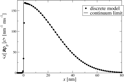
Figure 2: Dots: reset state $\left\langle x\left|{\mathcal{R}}\varrho_{\mathrm{p}}\right|x\right\rangle$ for a pure state $\varrho_{\mathrm{p}}=\left|\psi\right\rangle\left\langle\psi\right|$ with $\left|\psi\right\rangle$ the Gaussian wave packet of Eq. (31), $\Delta x=50~{}\mathrm{nm}$ and $v_{0}=1.79~{}\mathrm{m}/\mathrm{s}$; $\omega_{0}=2.38\times 10^{12}~{}\mathrm{s}^{-1}$, $\omega_{{}_{\mathrm{M}}}=4.6\,\omega_{0}$, $G=2.782\times 10^{3}~{}\mathrm{s}^{-1/2}$, $N=15$, and $\Delta t=100\;\omega_{0}^{-1}=4.185\times 10^{-11}~{}\mathrm{s}$. Solid line: reset state $A\,\left|\langle x\left|\Theta(\hat{x})\right|\psi\rangle\right|^{2}$ from Eq. (42) for the corresponding continuum limit. Up to small deviations around $x=0$, the reset states from the discrete and the continuum model are in very good agreement.

III.3 The continuum limit

We return to the general expression in Eq. (LABEL:reset_full). For simplicity we will assume in the following

$$\chi^{(j)}(\mathbf{x})\equiv\chi(\mathbf{x}),~{}~{}~{}~{}~{}j=1,\cdots,D.$$ (35)

In view of Eq. (9) and the remarks after Eq. (10) we neglect the $\gamma_{\boldsymbol{\ell}}^{(j)}$ terms. We introduce the collective correlation function

$$\kappa(\tau)\equiv\sum_{j}\sum_{\boldsymbol{\ell}}\left|g^{(j)}_{\boldsymbol{\ell}}\right|^{2}e^{-i\left(\omega_{\ell}-\widetilde{\omega}_{0}^{(j)}\right)\tau}.$$ (36)

Since we assume that the coupling constants are such that the Markov property holds in the continuum limit, i.e.,

$$\kappa(\tau)\approx 0~{}~{}~{}\mathrm{if}~{}~{}~{}\tau>\tau_{c}$$ (37)

for some small correlation time $\tau_{c}$, in the double integral of Eq. (LABEL:reset_full) only times with $t_{1}-t_{2}\leq\tau_{c}$ contribute, and if $\tau_{c}$ is small enough one can write

$$\chi[\hat{\mathbf{x}}(t_{1})]\approx\chi[\hat{\mathbf{x}}(t_{2})].$$ (38)

Then, with a change of variable, $\tau\equiv t_{1}-t_{2}$, the integration over $\tau$ can be extended to $\infty$ if $\tau_{c}\ll\Delta t$. Specializing the definition Eq. (II) to the case at hand, we put

$$A\equiv 2\mskip 1.0mu\mathrm{Re}\int_{0}^{\infty}d\tau\,\kappa(\tau)$$ (39)

and note that $A$ is given by the right side of Eq. (II) without the terms $\Gamma^{(j)}_{\mathrm{spon}}$ and $\chi^{(j)}({\mathbf{x}})$. One then obtains

$${\mathcal{R}}\varrho_{\mathrm{p}}\;\Delta t = A\,\int\limits_{0}^{\Delta t}dt_{1}e^{-\frac{i}{\hbar}H_{\mathrm{part}}(\Delta t-t_{1})}\chi(\hat{\mathbf{x}})e^{-\frac{i}{\hbar}H_{\mathrm{part}}t_{1}}\varrho_{\mathrm{p}}e^{\frac{i}{\hbar}H_{\mathrm{part}}t_{1}}\chi(\hat{\mathbf{x}})e^{\frac{i}{\hbar}H_{\mathrm{part}}(\Delta t-t_{1})}$$ (40)

$$= A\,\chi(\hat{\mathbf{x}})\varrho_{\mathrm{p}}\chi(\hat{\mathbf{x}})\;\Delta t+\mathcal{O}(\Delta t^{2}).$$

Hence, to first order in $\Delta t$, one finally has

$${\mathcal{R}}\varrho_{\mathrm{p}}=A\,\chi(\hat{\mathbf{x}})\varrho_{\mathrm{p}}\chi(\hat{\mathbf{x}})$$ (41)

for the state immediately after a detection.

${\mathcal{R}}$ is called the reset operation. If $\varrho_{\mathrm{p}}$ is a pure state, then the reset state is also a pure state. In particular, if $\varrho_{\mathrm{p}}=\left|\psi_{\mathrm{cond}}^{t}\right\rangle\left\langle\psi_{\mathrm{cond}}^{t}\right|$, then the reset state is given by the wave function

$$\left|\psi_{\mathrm{reset}}^{t}\right\rangle\equiv A^{1/2}\chi(\hat{\mathbf{x}})\left|\psi_{\mathrm{cond}}^{t}\right\rangle.$$ (42)

We note that this result is physically very reasonable since it means that right after a detection of the particle by a detector located in a specific region the particle is localized in that region. We also note that [see Eq. (23)]

$$\left\langle\psi_{\mathrm{reset}}^{t}\left|\psi_{\mathrm{reset}}^{t}\right.\right\rangle=w_{1}(t),$$ (43)

which is the probability density for the first detection.

We apply Eq. (42) to the continuum limit of the example of Subsection III.2. In that one-dimensional and single-spin case one has with Eqs. (30) and (36)

$$\kappa(\tau) = \omega_{{}_{\mathrm{M}}}|G|^{2}\sum_{n=1}^{N}\frac{1}{N}\frac{n}{N}e^{-i\omega_{{}_{\mathrm{M}}}\tau\,(n/N)+i\omega_{0}\tau}$$

$$\to \omega_{{}_{\mathrm{M}}}|G|^{2}\int_{0}^{1}d\xi\,\xi\,e^{-i\omega_{{}_{\mathrm{M}}}\tau\,\xi+i\omega_{0}\tau}\quad\mathrm{for}~{}N~{}\to~{}\infty.$$

Thus one obtains in the continuum limit

$$\kappa(\tau) = \frac{|G|^{2}}{\omega_{{}_{\mathrm{M}}}}\;\frac{\left(1+i\omega_{{}_{\mathrm{M}}}\tau\right)e^{-i(\omega_{{}_{\mathrm{M}}}-\omega_{0})\tau}-e^{i\omega_{0}\tau}}{\tau^{2}}$$

$$A = 2\pi\left|G\right|^{2}\,\frac{\omega_{0}}{\omega_{{}_{\mathrm{M}}}}\quad\mathrm{for}~{}\omega_{{}_{\mathrm{M}}}>\omega_{0}$$

$$\delta_{\mathrm{shift}} = 2\left|G\right|^{2}\left(\frac{\omega_{0}}{\omega_{{}_{\mathrm{M}}}}\ln\left[\frac{\omega_{0}}{\omega_{{}_{\mathrm{M}}}-\omega_{0}}\right]-1\right),$$ (45)

and $\tau_{\mathrm{c}}$ is of the order of $\omega_{0}^{-1}$. The resulting spatial probability density $A\,\left|\langle x\left|\Theta(\hat{x})\right|\psi\rangle\right|^{2}$ is plotted in Fig. 2 for the same initial state and same parameters as in the discrete case. The plots are in very good agreement.

We note that in the present model with $f_{\boldsymbol{\ell}}^{(j)}$ independent of $\mathbf{x}$ there is no explicit recoil on the particle from the created boson. This is in line with the original idea of a minimally invasive measurement. The absence of an explicit recoil distinguishes the present detector model from other models which are based on the direct interaction with the particle’s internal degrees of freedom. An example for such a model would be the detection by means of laser induced fluorescence. In that case, the reset state after the detection of the first fluorescence photon explicitely incorporates a recoil due to the momentum of the emitted photon Hegerfeldt (2003). It appears reasonable that in the present model no such recoil on the particle occurs: After all, the boson is emitted not by the particle but by the spin lattice. Hence, the recoil should be experienced by this lattice, rather than by the particle, similar to what occurs in the Mössbauer effect. Of course, the projection of the wave packet onto the detector region by means of the reset operation also changes the momentum distribution of the wave packet.

III.4 Subsequent time development

After detection of a boson, the further interaction of the particle with the detector depends on the particular choice of parameters of the detector model. The internal dynamics of the detector after the first spin flip has been investigated in detail in Refs. Schulman (1997); Gaveau and Schulman (1990); Schulman (1991). Based on these results, several choices are possible such that the amplification of the first spin flip will not significantly change the spatial wave function after the first spin flip, $\left|\psi_{\mathrm{reset}}^{t}\right\rangle$. This means that effectively only one reset operation, associated with the very first spin flip, has to be performed on the spatial wave function. Such “minimally invasive” detector models will be of interest if one is interested in actual quantum mechanical limitations of a passage-time measurement.

As a simple example, consider a ring of identical spins with nearest-neighbor interaction,

$$\omega_{0}^{(j)}\equiv\omega_{0}\quad\mathrm{and}\quad\omega_{J}^{(jk)}\equiv\omega_{J}\;\delta_{j+1,k}$$ (46)

with $\delta_{j+1,k}$ Kronecker’s $\delta$, $\chi^{(j)}(\mathbf{x})\equiv\chi(\mathbf{x})$ as before, and $j=D+1$ identified with $j=1$. The rate for the neighbors of the first-flipped spin to flip into their ground state is denoted by $A_{1}(\mathbf{x})$ and is given by the right side of Eq. (II), but with $\widetilde{\omega}_{0}$ replaced by $\omega_{0}$ since the ferromagnetic forces on these neighboring spins cancel. Choosing parameters as, e.g., $\omega_{0}\gg\widetilde{\omega}_{0}$ and $\Gamma,~{}\Gamma_{\mathrm{spon}}$ independent of $\omega_{\ell}$ as well as $c(\omega_{\ell})\equiv c_{0}$, one has $A_{1}\gg A$. By a kind of domino effect the whole ring flips into the ground state; the mean time needed for this given by $D/2A_{1}$ Schulman (1997); Gaveau and Schulman (1990); Schulman (1991). If this time is very short, as one can achieve by making $\omega_{0}$ large (while $\widetilde{\omega}_{0}$ remains small to prevent spontaneous spin flips before the first particle-induced spin flip), the reset operations associated with these subsequent spin flips will not significantly change the particle’s state since the wave function has been projected onto the detector by the first reset operation already.

Another possibility to prevent the spatial wave function from being changed by the amplification process would be to couple only one spin to the particle, by choosing $g_{\boldsymbol{\ell}}^{(j)}=g_{\boldsymbol{\ell}}\,\delta_{j,j_{0}}$ in Eq. (8). (In fact, this is the de facto setup of the detector actually investigated in Refs. Gaveau and Schulman (1990); Schulman (1991, 1997): Effectively only one spin couples to the particle, and subsequently the other spins flip spontaneously, i.e., without particle-enhanced spin-bath coupling.)

IV Application to passage times

IV.1 General setup

We now consider two detectors separated by some distance. As indicated in the preceding section, we assume that the amplification of the first spin flip to a macroscopic event is very fast and does not change the spatial wave function. Thus, we take the probability density $w_{1}(t)$ [Eq. (23)] for the first spin flip to be the “measured arrival-time distribution” and $\left|\psi_{\mathrm{reset}}^{t}\right\rangle$ [Eq. (42)] as the particle’s state after the detection. Then, the joint probability density for the first detector detecting the particle at $T$ and the second one detecting it at $T+\tau$ is given by

$$G(T,T+\tau)=w_{1}^{(1)}\left(T;\left|\psi_{0}\right\rangle\right)\;w_{1}^{(2)}\left(\tau;\frac{\left|\psi_{\mathrm{reset}}^{T}\right\rangle}{\left\|\left|\psi_{\mathrm{reset}}^{T}\right\rangle\right\|}\right),$$ (47)

where the superscripts indicate the detector under consideration and the second argument is the initial state for which the respective probability density is calculated. Since $w_{1}$ is bilinear in the wave function [see Eq. (23)], this simplifies to

$$G(T,T+\tau)=w_{1}^{(2)}\left(\tau;\left|\psi_{\mathrm{reset}}^{T}\right\rangle\right)$$ (48)

by Eq. (43). The desired measured passage-time distribution is then given by integration over the entry time $T$:

$$G(\tau)=\int dT\,w_{1}^{(2)}\left(\tau;\left|\psi_{\mathrm{reset}}^{T}\right\rangle\right).$$ (49)

IV.2 Numerical example

In order to investigate basic features of a quantum passage-time distribution obtained from the detector model in the continuum limit and in the above measurement scheme, we consider as a simple example a cesium atom in one dimension. The initial wave packet is prepared in the remote past far away from the detector such that the free wave packet (with no detectors present) would be described at $t=0$ by a Gaussian minimal uncertainty packet around $x=0$ with $\Delta x=1\mu\mathrm{m}$ and average velocity $v_{0}=0.717\mathrm{cm/s}$. Each of the two identical detectors is described in the continuum limit by an absorbing potential $-iV=-i\hbar A/2$ extending from $0$ to $20\mu\mathrm{m}$ or $100\mu\mathrm{m}$ to $120\mu\mathrm{m}$, resp., where we consider three different examples $A=1.4337\times 10^{3}~{}\mathrm{s}^{-1},2.3895\times 10^{3}~{}\mathrm{s}^{-1},2.3895\times 10^{4}~{}\mathrm{s}^{-1}$. These parameters are chosen in such a way that transmission and reflection without detection, which are typical for imaginary potentials Allcock (1969) and have been extensively studied in the framework of quantum arrival times Damborenea et al. (2002); Hegerfeldt et al. (2003); Navarro et al. (2003); Damborenea et al. (2003), play no significant role. Consequently, all distributions shown in the following are normalized to 1 to a good approximation. The passage-time distributions, calculated as described in Section IV.1, are shown in Fig. 3.

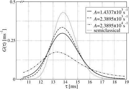
Figure 3: Passage-time distributions calculated from the detector model in the continuum limit for three different values of the rate $A$ for the first spin flip in the presence of the particle, all other parameters kept fixed; for comparison, the dotted line shows the passage-time distribution for an ensemble of classical particles which have the same momentum distribution as the initial wave packet.

It is seen that small and large values of $A$ give rise to rather broad distributions, while the intermediate value yields a narrower one. The reason for the broad distribution arising for small $A$ can be understood by looking at the arrival-time distribution measured by the first detector (see Fig. 4): It is already this distribution which is rather broad for small $A$.

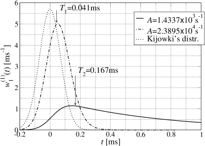
Figure 4: Arrival-time distributions as obtained from the first detector. The detector with small $A$ gives a broad distribution indicating poor quality of this measurement. Enlarging $A$ carefully (to avoid reflection), one may approach Kijowski’s axiomatically derived arrival-time distribution at $x=0$ (dotted line).

Physically, small $A$ means that the detector is responding only slowly to the presence of the particle; the undetected amplitude $\left|\psi_{\mathrm{cond}}^{t}\right\rangle$ decays only slowly, yielding a broad arrival-time distribution at each of the two detectors and consequently a broad passage-time distribution. In other words, the poor quality of the passage-time measurement arises from the poor quality of the individual arrival-time measurements. The measurement of the arrival time, however, can be improved by making $A$ large, that is, by making the detector responding faster to the presence of the particle. In Fig. 4 it is seen, e.g., that for $A=2.3895\times 10^{4}~{}\mathrm{s}^{-1}$ one comes much closer to Kijowski’s arrival-time distribution; this in turn is known to have minimum standard deviation among all those distributions fulfilling certain axioms transferred to quantum mechanics from classical arrival-time distributions Kijowski (1974), and thus provides a sort of “ideal distribution.”

While the broad passage-time distribution for small $A$ can be understood simply as due to the poor quality of the individual measurements, the broad distribution for large $A$ is more interesting. It can be understood looking at the reset state immediately after the detection by the first detector. Of course, this reset state depends on the instant of time when the detection took place; as an example, we consider detection times $T_{1}=0.041~{}\mathrm{ms}$ if $A=2.3895\times 10^{4}~{}\mathrm{s}^{-1}$ and $T_{2}=0.167~{}\mathrm{ms}$ if $A=1.4337\times 10^{3}~{}\mathrm{s}^{-1}$, which are close to the maximum of the respective probability distribution $w_{1}(t)$ (see Fig. 4). The reset states and the free packet at the respective times are shown in Fig. 5.

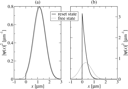
Figure 5: The normalized reset state in position space immediately after a detection at (a) $T_{2}=0.167~{}\mathrm{ms}$ (with $A=1.4337\times 10^{3}~{}\mathrm{s}^{-1}$) and at (b) $T_{1}=0.041~{}\mathrm{ms}$ (with $A=2.3895\times 10^{4}\mathrm{s}^{-1}$), compared with the free wave packet at the respective instance of time (dotted line). The fast detection in case (b) has a strong impact on the wave function.

It is seen that the fast detection has a strong impact on the wave function. Large $A$ means that $\left|\psi_{\mathrm{cond}}^{t}\right\rangle$, in particular that part of $\left|\psi_{\mathrm{cond}}^{t}\right\rangle$ which overlaps with the detector, decays very fast. But since the reset state (42) immediately after the detection is essentially the projection of $\left|\psi_{\mathrm{cond}}^{t}\right\rangle$ onto the detector region, the fast decay of this overlap yields a reset state which is very narrow in position space, located at the very beginning of the detector. Thus, by the Heisenberg uncertainty relation, it is very broad in momentum space as can be seen in Fig. 6. It is intuitively clear that such a broad momentum distribution immediately after the measurement of the entry time by the first detector yields a broad passage-time distribution. So the broad passage-time distribution in case of large $A$ is due to the strong distortion of the wave function by the first measurement. Since the broad momentum distribution of the typical reset states in this case is enforced by the Heisenberg uncertainty relation, this is a pure quantum effect.

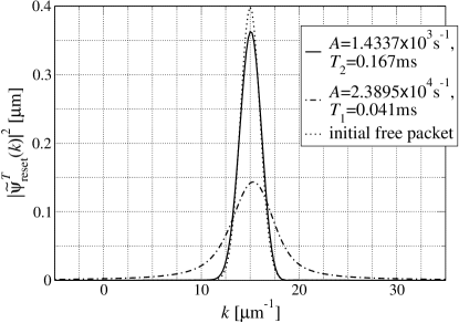
Figure 6: Momentum distributions of reset states immediately after a detection at $T_{2}=0.167~{}\mathrm{ms}$ (solid line, with $A=1.4337\times 10^{3}~{}\mathrm{s}^{-1}$) and at $T_{1}=0.041~{}\mathrm{ms}$ (dash-dotted line, with $A=2.3895\times 10^{4}~{}\mathrm{s}^{-1}$), compared to the momentum distribution of the initial wave packet (dotted line). The fast detection in the latter case leads to a strong broadening of the momentum distribution.

V Width of the passage-time density

In Refs. Peres (1980); Alonso et al. (2003) a measurement scheme for passage times was investigated, based on the (semi-) continuous coupling of a particle to a clock. It was argued in these references that the precision of the measurement behaves like $E^{-1}$ where $E$ denotes the kinetic energy of the particle. One now may wonder whether or not the $E^{-1}$ behavior is a fundamental quantum limit for measuring passage times. We argue that this is not the case since the present measurement scheme by means of two spatially separated detectors yields, for optimal parameter choices, passage-time densities with widths behaving like $E^{-3/4}$. Thus, for low energies, we have an example which breaks the $E^{-1}$ limitation of the clock model.

V.1 Estimating the precision

In this subsection we give an estimate for the width of the passage-time density obtained from the present measurement scheme. We assume that the detectors can be described by the continuum limit and that transmission and reflection without detection are negligible. This assumption is justified in the examples of the preceding section, which employed rectangular sensitivity functions. It can also be justified in general if one drops the restriction to rectangular sensitivity functions $\chi(x)$ opt .

Considering particles with mean velocity $v_{0}$, the detector is assumed to be constructed in such a way that the first detection occurs with high probability in a spatial interval of length $L$. The length $L$ is related to $A$ of Eq. (39), an average detection rate, $L$ being of the order of $v_{0}/A$. The length $L$ imposes an upper limit on the width of the reset state in position space,

$$\Delta x_{\mathrm{reset}}\leq L\approx v_{0}/A.$$ (50)

By the Heisenberg uncertainty relation, this immediately yields a lower bound for the width $\Delta p_{\mathrm{reset}}$ of the reset state in momentum space,

$$\Delta p_{\mathrm{reset}}\geq\hbar/2\Delta x_{\mathrm{reset}}\geq\hbar/2L.$$ (51)

Note that this is only a very rough estimate, without taking into account details of the actual wave packet. If the incident wave packet is very narrow in position space, then $\Delta x_{\mathrm{reset}}$ also may be much smaller than $L$, and consequently $\Delta p_{\mathrm{reset}}$ may be much larger than $\hbar/2L$. Also, the reset state may be far from being a Gaussian, and then already the first inequality in Eq. (51) may underestimate the width of $\Delta p_{\mathrm{reset}}$ seriously.

Let $\Delta\tau$ denote the width of the measured passage-time distribution. There are several contributions to this width. First, a particle with velocity $v_{0}$ takes the time $\tau=d/v_{0}$ to travel the distance $d$ between the two detectors, and therefore the width of the reset state in position space contributes

$$\Delta\tau_{\mathrm{reset},x}=\Delta x_{\mathrm{reset}}/v_{0}$$ (52)

to $\Delta\tau$. Second, the width in momentum space contributes according to

$$\Delta\tau_{\mathrm{reset},p}=\frac{\Delta p_{\mathrm{reset}}}{mv_{0}}\frac{d}{v_{0}}\geq\frac{\hbar}{2\Delta x_{\mathrm{reset}}}\frac{d}{mv_{0}^{2}}.$$ (53)

Third, the width of the delay, $\Delta\tau_{\mathrm{delay}}$, for the first detection due to the spin-boson interaction is roughly

$$\Delta\tau_{\mathrm{delay}}=1/A\approx L/v_{0}.$$ (54)

An estimate for the width of the passage-time distribution is given by the sum of these contributions, where $\Delta\tau_{\mathrm{delay}}$ has to be counted twice since it arises in both detectors:

$$\Delta\tau = 2\Delta\tau_{\mathrm{delay}}+\Delta\tau_{\mathrm{reset},x}+\Delta\tau_{\mathrm{reset},p}$$ (55)

$$\gtrsim 2/A+\Delta x_{\mathrm{reset}}/v_{0}+\hbar d/2mv_{0}^{2}\Delta x_{\mathrm{reset}}.$$

From this estimate it is again seen that both small as well as large values of $A$, i.e., both slow as well as fast detectors, lead to rather broad passage-time distributions (due to $\Delta\tau_{\mathrm{delay}}\sim 1/A$ and $\Delta\tau_{\mathrm{reset},p}\sim 1/\Delta x_{\mathrm{reset}}\sim 1/L\sim A$, respectively).

V.2 Optimal parameters

Having established the general estimate for $\Delta\tau$ in Eq. (55), we now turn to the task of finding optimal parameters, minimizing $\Delta\tau$. We are interested in measuring the passage time through a spatial interval of length $d$, the distance between the starting points of the two detectors, which we regard as fixed. First, we consider given detectors, i.e., a given detection rate, $A$. Again, particles with mean velocity $v_{0}$ would be detected within an interval with length $L$ given approximately by $L\approx v_{0}/A$. This means that the velocities must not be too large since in order to avoid undetected transmission $L$ must not exceed the actual length of the detector (and in particular $L$ must not exceed $d$). Quantum effects, however, are expected to play a role for slow particles while fast particles may be treated classically, hence this is not a serious drawback.

We assume that the reset state is a Gaussian wave packet, or at least close to a Gaussian, so that in the second line of Eq. (55) the approximate equality holds,

$$\Delta\tau\approx 2/A+\Delta x_{\mathrm{reset}}/v_{0}+\hbar d/2mv_{0}^{2}\Delta x_{\mathrm{reset}}.$$ (56)

We note that $2/A$ is a purely detector-related quantity, while the remaining contribution to $\Delta\tau$ is determined by the shape of the reset state only. We will first optimize this latter quantity. For given particles with given mean velocity, i.e., $m$ and $v_{0}$ fixed, this is minimal for

$$\Delta x_{\mathrm{reset}}^{\mathrm{opt}}=\sqrt{\hbar d/2mv_{0}}.$$ (57)

Substituting this into Eq. (56) and writing $E=mv_{0}^{2}/2$ for the kinetic energy of the incident particles yields

$$\Delta\tau_{\mathrm{opt;~{}reset}}\approx 2/A+\sqrt{\hbar d\sqrt{m/2}}\;E^{-3/4}.$$ (58)

The subscript “$\mathrm{opt;~{}reset}$” indicates that only the reset state was optimized while the detection rate $A$ was considered as a given quantity.

Aiming at optimizing also the detection rate $A$ for minimal $\Delta\tau$, one would like to choose $A$ as large as possible in order to reduce the $2/A$ contribution to $\Delta\tau$. However, one has to take into account that the width of the reset state is bounded by Eq. (50). Thus, given $d$, $m$, and $v_{0}$, the decay rate must be at most of the order of $v_{0}/\Delta x_{\mathrm{reset}}^{\mathrm{opt}}$ with $\Delta x_{\mathrm{reset}}^{\mathrm{opt}}$ as in Eq. (57). In fact, we may choose the incoming state such that it forms a Gaussian minimal uncertainty packet at the starting point of the first detector with width in position space

$$\Delta x=\Delta x_{\mathrm{reset}}^{\mathrm{opt}}=\sqrt{\hbar d/2mv_{0}},$$ (59)

and choose further

$$A\approx v_{0}/2\Delta x=\sqrt{m/2\hbar d}\;v_{0}^{3/2}.$$ (60)

We note that, by this parameter choice, yet another requirement of a good measurement scheme is fulfilled: The detection by the first detector will not change the wave function too strongly. The reset operation after this detection is essentially a projection onto the detector region, and the detection is slow enough that at typical detection times most of the wave packet overlaps with the detector, hence the projection does not change the wave function too much. Thus, the reset state will be close to a Gaussian wave packet with width $\Delta x=\Delta x_{\mathrm{reset}}^{\mathrm{opt}}$. Substituting Eq. (60) into Eq. (58) finally yields

$$\Delta\tau_{\mathrm{opt}}\approx\sqrt{5\hbar d\sqrt{m/2}}\;E^{-3/4}.$$ (61)

We stress that, independent of the detection rate $A$, the optimal energy dependence of $\Delta\tau$ is limited to $E^{-3/4}$ already by the dependence of $\Delta\tau$ on the width of the reset state in position space, $\Delta\tau_{\mathrm{reset},x}\sim\Delta x_{\mathrm{reset}}$ [Eq. (52)], and on its width in momentum space, $\Delta\tau_{\mathrm{reset},p}\sim\Delta p_{\mathrm{reset}}\sim 1/\Delta x_{\mathrm{reset}}$ [see Eq. (53)].

For the example of a cesium atom with $v_{0}=0.717~{}\mathrm{cm/s}$ and a distance of $d=100~{}\mu\mathrm{m}$ between the detectors (with rectangular sensitivity function) of the preceding section, optimal values would be according to Eqs. (57) and (60)

$$\Delta x_{\mathrm{opt}}=1.83~{}\mu\mathrm{m},\;\;\text{and}\;\;A_{\mathrm{opt}}=1.959\times 10^{3}~{}\mathrm{s}^{-1}.$$ (62)

Considering the wave packet with $\Delta x=1~{}\mu\mathrm{m}$ actually investigated in the examples, the optimal decay rate according to Eq. (60) would be $A_{\mathrm{opt}}(\Delta x=1~{}\mu\mathrm{m})=3.585\times 10^{3}~{}\mu\mathrm{s}^{-1}$. This is consistent with the observation that the example with $A$ closest to $A_{\mathrm{opt}}(\Delta x=1~{}\mu\mathrm{m})$ yields the narrowest distribution.

Summary

We have investigated the continuum limit of a fully quantum mechanical spin-boson model for the detection of a moving particle and its application to passage-time measurements. The continuum limit has been derived under the condition that the spin-boson interaction satisfies the Markov property, an assumption that was explicitly verified in Ref. Hegerfeldt et al. (2006). Analytical expressions for the state immediately after the first detection have been obtained, and for an example with a simplified detector model and 15 boson modes it was shown numerically that the continuum limit is in very good agreement with the discrete model. Further, analytical expressions for the passage-time distribution have been obtained, and numerical examples for passage-time measurements have been discussed. Detectors with a very slow response yield broad distributions, due to the poor quality of the individual measurements, and so do very fast detectors, due to the strong distortion of the particle’s wave function by the measurement. Intermediate detectors yield narrower distributions. The optimal precision of the present measurement scheme has been estimated to behave like $E^{-3/4}$, where $E$ is the kinetic energy of the incident particle. For slow particles this is better than, and in contrast to, a scheme based on quantum clocks which yields an $E^{-1}$ behavior.

References

- Szriftgiser et al. (1996) P. Szriftgiser, D. Guéry-Odelin, M. Arndt, and J. Dalibard, Phys. Rev. Lett. 77, 4 (1996).
- Smith (1960) F. T. Smith, Phys. Rev. 118, 349 (1960).
- Sokolovski and Baskin (1987) D. Sokolovski and L. M. Baskin, Phys. Rev. A 36, 4604 (1987).
- Jaworski and Wardlaw (1988) W. Jaworski and D. M. Wardlaw, Phys. Rev. A 37, 2843 (1988).
- Muga et al. (1992) J. G. Muga, S. Brouard, and R. Sala, Phys. Lett. A 167, 24 (1992).
- Baz’ (1967) A. Baz’, Sov. J. Nucl. Phys. 5, 182 (1967).
- Rybachenko (1967) V. Rybachenko, Sov. J. Nucl. Phys. 5, 635 (1967).
- Balcou and Dutriaux (1997) P. Balcou and L. Dutriaux, Phys. Rev. Lett. 78, 851 (1997).
- Salecker and Wigner (1958) H. Salecker and E. P. Wigner, Phys. Rev. 109, 571 (1958).
- Peres (1980) A. Peres, Am. J. Phys. 48, 552 (1980).
- Alonso et al. (2003) D. Alonso, R. Sala Mayato, and J. G. Muga, Phys. Rev. A 67, 032105 (2003).
- Hauge and Støvneng (1989) E. H. Hauge and J. A. Støvneng, Rev. Mod. Phys. 61, 917 (1989).
- Landauer and Martin (1994) R. Landauer and T. Martin, Rev. Mod. Phys. 66, 217 (1994).
- Schulman and Ziolkowski (1989) L. S. Schulman and R. W. Ziolkowski, in Path Integrals from meV to MeV, edited by V. Sa-yakanit, W. Sritrikool, J.-O. Berananda, M. C. Gutzwiller, A. Inomata, S. Lundqvist, J. R. Klauder, and L. Schulman (World Scientific, Singapore, 1989), pp. 253–278, proceedings of an international conference held in Bangkok, January 1989.
- Sokolovski and Baskin (1987) D. Sokolovski and L. M. Baskin, Phys. Rev. A 36, 4604 (1987).
- Yamada (1999) N. Yamada, Phys. Rev. Lett. 83, 3350 (1999).
- Hegerfeldt et al. (2006) G. C. Hegerfeldt, J. T. Neumann, and L. S. Schulman, J. Phys. 39, 14447 (2006). A simplified version of the detector model has been investigated by J. J. Halliwell in Ref. Halliwell (1999).
- Schulman (1997) L. S. Schulman, Time’s arrows and quantum measurement (Cambridge University Press, Cambridge, 1997).
- Gaveau and Schulman (1990) B. Gaveau and L. S. Schulman, J. Stat. Phys. 58, 1209 (1990).
- Schulman (1991) L. S. Schulman, Ann. Phys. (NY) 212, 315 (1991).
- (21) G. C. Hegerfeldt and T. S. Wilser, in: Classical and Quantum Systems. Proceedings of the Second International Wigner Symposium, July 1991, edited by H. D. Doebner, W. Scherer, and F. Schroeck (World Scientific, Singapore, 1992), p. 104; G. C. Hegerfeldt, Phys. Rev. A 47, 449 (1993); G. C. Hegerfeldt and D. G. Sondermann, Quantum Semiclass. Opt. 8, 121 (1996). For a review cf. Plenio and Knight (1998). The quantum jump approach is essentially equivalent to the Monte-Carlo wavefunction approach Dalibard et al. (1992), and to the quantum trajectories of H. Carmichael Carmichael (1993).
- Hegerfeldt (1993) G. C. Hegerfeldt, Phys. Rev. A 47, 449 (1993).
- von Neumann (1932) J. von Neumann, Mathematische Grundlagen der Quantenmechanik (Springer, Berlin, 1932), [English translation: Mathematical Foundations of Quantum Mechanics (Princeton University Press, Princeton, 1955)], Chap. V.1.
- Lüders (1951) G. Lüders, Ann. Phys. (Leipzig) 443, 322 (1951).
- Hegerfeldt (2003) G. C. Hegerfeldt, in Irreversible Quantum Dynamics, edited by F. Benatti and R. Floreanini (Springer LNP 622, 2003), pp. 233 – 242.
- Allcock (1969) G. R. Allcock, Ann. Phys. (NY) 53, 253 (1969); 53, 286 (1969); 53, 311 (1969).
- Damborenea et al. (2002) J. A. Damborenea, I. L. Egusquiza, G. C. Hegerfeldt, and J. G. Muga, Phys. Rev. A 66, 052104 (2002).
- Hegerfeldt et al. (2003) G. C. Hegerfeldt, D. Seidel, and J. G. Muga, Phys. Rev. A 68, 022111 (2003).
- Navarro et al. (2003) B. Navarro, I. L. Egusquiza, J. G. Muga, and G. C. Hegerfeldt, J. Phys. B 36, 3899 (2003).
- Damborenea et al. (2003) J. A. Damborenea, I. L. Egusquiza, G. C. Hegerfeldt, and J. G. Muga, J. Phys. B: At. Mol. Opt. Phys. 36, 2657 (2003).
- Kijowski (1974) J. Kijowski, Rep. Math. Phys. 6, 361 (1974).
- (32) By means of inverse scattering techniques it has been shown Muga et al. (1995); Palao et al. (1998) that for a given energy range an optimized absorbing potential can be constructed which almost completely absorbs wave packets of this energy range in a very short spatial interval. Such a potential can then be considered as a continuum limit of a discrete spin-boson detector.
- Halliwell (1999) J. J. Halliwell, Progr. Theor. Phys. 102, 707 (1999).
- Plenio and Knight (1998) M. B. Plenio and P. L. Knight, Rev. Mod. Phys. 70, 101 (1998).
- Dalibard et al. (1992) J. Dalibard, Y. Castin, and K. Mølmer, Phys. Rev. Lett. 68, 580 (1992).
- Carmichael (1993) H. Carmichael, An Open System Approach to Quantum Optics, vol. m 18 of LNP (Springer Verlag, Berlin, 1993).
- Muga et al. (1995) J. G. Muga, S. Brouard, and D. Macías, Ann. Phys. (NY) 240, 351 (1995).
- Palao et al. (1998) J. P. Palao, J. G. Muga, and R. Sala, Phys. Rev. Lett. 80, 5469 (1998).