Maximally polarized states for quantum light fields

Abstract

degree of polarization of a quantum state can be defined as its Hilbert-Schmidt distance to the set of unpolarized states. We demonstrate that the states optimizing this degree for a fixed average number of photons $\bar{N}$ present a fairly symmetric, parabolic photon statistics, with a variance scaling as $\bar{N}^{2}$. Although no standard optical process yields such a statistics, we show that, to an excellent approximation, a highly squeezed vacuum can be considered as maximally polarized.

A number of key concepts in quantum optics can be concisely quantified in terms of distance measures. The notions of nonclassicality nonclass , entanglement entang , information accinf , localization local , or polarization pol , to cite only a few relevant examples, have been systematically formulated within this framework. The rationale behind this is quite clear: once we have identified a convex set with the desired physical properties (classicality, separability, etc.), the distance determines the distinguishability of a state with respect to that set Wootters81 . Apart from its conceptual simplicity, this procedure avoids many undesired problems that can arise in more standard approaches.

Irrespective of our particular choice for the distance, a natural question emerges: what states maximize the corresponding measure. A good deal of effort has been devoted to characterize maximally nonclassical or entangled states. However, as far as we know, maximally polarized states have been not considered thus far, except for some trivial cases. It is precisely the purpose of this Letter to fill this gap, providing a complete description of such states, as well as feasible experimental schemes for their generation.

Let us start by briefly recalling some basic concepts about quantum polarization. We assume a monochromatic plane wave propagating in the $z$ direction, whose electric field lies in the $xy$ plane. Under these conditions, the field can be fully represented by two complex amplitude operators, denoted by $\hat{a}_{H}$ and $\hat{a}_{V}$ when using the basis of linear (horizontal and vertical) polarizations. They obey the standard bosonic commutation relations $[\hat{a}_{j},\hat{a}_{k}^{\dagger}]=\delta_{jk}$, with $j,k\in\{H,V\}$. The Stokes operators are then introduced as the quantum counterparts of the classical variables Stokes , namely

$$\hat{S}_{0}=\hat{a}^{\dagger}_{H}\hat{a}_{H}+\hat{a}^{\dagger}_{V}\hat{a}_{V}\,,\qquad\hat{S}_{1}=\hat{a}^{\dagger}_{H}\hat{a}_{V}+\hat{a}^{\dagger}_{V}\hat{a}_{H}\,,$$

(1)

$$\hat{S}_{2}=i(\hat{a}_{H}\hat{a}^{\dagger}_{V}-\hat{a}^{\dagger}_{H}\hat{a}_{V})\,,\qquad\hat{S}_{3}=\hat{a}^{\dagger}_{H}\hat{a}_{H}-\hat{a}^{\dagger}_{V}\hat{a}_{V}\,,$$

and their mean values are precisely the Stokes parameters $(\langle\hat{S}_{0}\rangle,\langle\hat{\mathbf{S}}\rangle)$, where $\hat{\mathbf{S}}^{T}=(\hat{S}_{1},\hat{S}_{2},\hat{S}_{3})$ and the superscript $T$ indicates the transpose. One immediately gets that the Stokes operators satisfy the commutation relations of the algebra su(2): $[\hat{S}_{1},\hat{S}_{2}]=2i\hat{S}_{3}$, and cyclic permutations. Moreover, since $[\hat{\mathbf{S}},\hat{S}_{0}]=0$, each energy manifold (with a fixed number of photons) can be treated separately. To bring out this point more clearly, it is advantageous to relabel the standard two-mode Fock basis $|n\rangle_{H}\otimes|m\rangle_{V}$ in the form

$$|N,k\rangle=|k\rangle_{H}\otimes|N-k\rangle_{V},\qquad k=0,1,\ldots,N.$$ (2)

These states span an invariant subspace of dimension $N+1$, and the operators $\hat{\mathbf{S}}$ act therein as an angular momentum $N/2$.

Any (linear) polarization transformation is generated by the Stokes operators (Maximally polarized states for quantum light fields). However, $\hat{S}_{0}$ induces only a common phase shift that does not change the polarization state and can thus be omitted. Therefore, we restrict ourselves to the SU(2) transformations, generated by $\mathbf{S}$. Since $\hat{S}_{1}$ is related to $\hat{S}_{2}$ and $\hat{S}_{3}$ by the commutation relations, only these two generators suffice. It is well known that $\hat{S}_{2}$ generates rotations around the direction of propagation, whereas $\hat{S}_{3}$ represents differential phase shifts between the modes. It follows then that any polarization transformation can be realized with linear optics: phase plates and rotators.

Although a precise defintion of polarized light at the quantum level may be controversial Klyshko96 , there is a wide consensus unpol in viewing unpolarized states as the only ones that remain invariant under any polarization transformation. It turns out that the density operator of these states can be written as

$$\hat{\sigma}=\sum_{N=0}^{\infty}p_{N}\left(\frac{1}{N+1}\ |N,k\rangle\langle N,k|\right)\,,$$ (3)

where $p_{N}$ is the two-mode photon-number distribution. Therefore, $\hat{\sigma}$ appears as diagonal in every subspace, with coefficients that guarantee the unit trace condition.

According to our previous discussion, it seems natural to quantify the degree of polarization of a state represented by the density operator $\hat{\varrho}$ as $\mathbb{P}(\hat{\varrho})\propto\inf_{\hat{\sigma}\in\mathcal{U}}D(\hat{\varrho},\hat{\sigma})$, where $\mathcal{U}$ denotes the convex set of unpolarized states of the form (3) and $D(\hat{\varrho},\hat{\sigma})$ is any measure of distance between the two density matrices $\hat{\varrho}$ and $\hat{\sigma}$. The degree $\mathbb{P}(\hat{\varrho})$ must be normalized to the unity and satisfy some requirements motivated by both physical and mathematical concerns entang . There are numerous nontrivial choices for $D(\hat{\varrho},\hat{\sigma})$: we shall consider here the Hilbert-Schmidt metric $D_{\mathrm{HS}}(\hat{\varrho},\hat{\sigma})=||\hat{\varrho}-\hat{\sigma}||_{2}^{2}=\mathop{\mathrm{Tr}}\nolimits[(\hat{\varrho}-\hat{\sigma})^{2}]$ because is the simplest one for computational purposes and allows us to get an analytic form of the degree of polarization

$$\mathbb{P}(\hat{\varrho})=\mathop{\mathrm{Tr}}\nolimits(\hat{\varrho}^{2})-\sum_{N=0}^{\infty}\frac{p_{N}^{2}}{N+1}\,,$$ (4)

which is determined by the purity $0<\mathop{\mathrm{Tr}}\nolimits(\hat{\varrho}^{2})\leq 1$ and the photon-number distribution $p_{N}$.

It is clear from Eq. (4) that for the states living in the manifold with exactly $N$ photons, the optimum is reached for pure states [for which $\mathop{\mathrm{Tr}}\nolimits(\hat{\varrho}^{2})=1$]. In fact, all such pure states have the same degree of polarization:

$$\mathbb{P}_{N}=\frac{N}{N+1}\sim 1-\frac{1}{N}\,,$$ (5)

where the last expression, showing the typical scaling $N^{-1}$, holds when $N\gg 1$. In particular, the important SU(2) coherent states on the Poincaré sphere Per86

$$|N,\theta,\phi\rangle=\sum_{k=0}^{N}C_{k}(\theta,\phi)\ |N,k\rangle\,,$$ (6)

with coefficients

$$C_{k}(\theta,\phi)=\left(\begin{array}[]{c}N\\ k\end{array}\right)^{1/2}\left(\sin\frac{\theta}{2}\right)^{N-k}\left(\cos\frac{\theta}{2}\right)^{k}e^{-ik\phi}$$ (7)

are such $N$-photon states.

However, this scaling law $N^{-1}$ can be easily surpassed. Perhaps the simplest example is when both modes are in (quadrature) coherent states, we denote by $|\alpha_{H},\alpha_{V}\rangle$. By reparametrizing the amplitudes as $\alpha_{H}=e^{-i\phi/2}\sqrt{\bar{N}}\sin(\theta/2)$ and $\alpha_{V}=e^{i\phi/2}\sqrt{\bar{N}}\cos(\theta/2)$, we can express them as

$$|\alpha_{H},\alpha_{V}\rangle=\sum_{N=0}^{\infty}e^{-\bar{N}/2}\frac{\bar{N}^{N/2}}{\sqrt{N!}}\,|N,\theta,\phi\rangle\,,$$ (8)

where $\bar{N}=|\alpha_{H}|^{2}+|\alpha_{V}|^{2}$ is the average number of photons. Since $p_{N}$ is a Poissonian with mean value $\bar{N}$, one can perform the sum in (4), with the result

$$\mathbb{P}_{\mathrm{coh}}=1-\frac{I_{1}(2\bar{N})}{\bar{N}}e^{-2\bar{N}}\sim 1-\frac{1}{2\sqrt{\pi}\bar{N}^{3/2}}\,.$$ (9)

where $I_{1}(z)$ is the modified Bessel function and the last equality is valid for $\bar{N}\gg 1$.

In consequence, we are led to find optimum states for a fixed average number of photons $\bar{N}$. Obtaining the whole optimum distribution $p_{N}$ in (4) is exceedingly difficult, since it involves optimizing over an infinite number of variables. Our strategy to attack this problem is to truncate the Hilbert space and consider only photon numbers up to some value $D$, where we take the limit $D\rightarrow\infty$ at the end. In this truncated space, we need to find the states that maximize (4) with the constraints

$$p_{N}\geq 0,\qquad\sum_{N=0}^{D}p_{N}=1,\qquad\sum_{N=0}^{D}N\ p_{N}=\bar{N}.$$ (10)

It is clear that the optimum must be again pure states. If we introduce the notations $p^{T}=(p_{0},p_{1},\ldots,p_{D})$ and $H=2\ \mathrm{diag}[1,1/2,\ldots,1/(D+1)]$, the task can be thus recast as

minimize $$\frac{1}{2}p^{T}Hp$$

subject to $$Ap=b,$$

$$p\geq 0,$$

where

$$b=\left(\begin{array}[]{c}1\\ \bar{N}\\ \end{array}\right),\qquad A=\left(\begin{array}[]{ccccc}1&1&1&\cdots&1\\ 0&1&2&\cdots&D\\ \end{array}\right).$$ (12)

We deal then with a quadratic programming problem that, in addition, is convex, because $H$ is positive definite Boyd04 . The optimum point exists and it is unique: in fact, there are numerous algorithms that compute this optimum in a quite efficient manner. Alternatively, we may try to determine it analytically by incorporating the constraints by the method of Lagrange multipliers. The functional to be minimized is

$$\mathcal{L}(p,\lambda)=\frac{1}{2}p^{T}Hp-\lambda^{T}(Ap-b)\,.$$ (13)

The first-order optimality conditions $\nabla\mathcal{L}(p,\lambda)=0$ together with the initial equality constraint, give the system of linear equations

$$\left(\begin{array}[]{cc}H&-A^{T}\\ A&0\end{array}\right)\left(\begin{array}[]{c}p\\ \lambda\end{array}\right)=\left(\begin{array}[]{c}0\\ b\end{array}\right)\,,$$ (14)

whose formal solution is

$$\lambda=(AH^{-1}A^{T})^{-1}b\,,\qquad p=H^{-1}A^{T}\lambda\,.$$ (15)

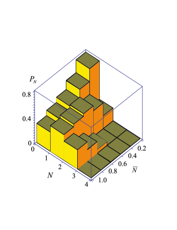
Figure 1: Optimum distribution $p_{N}$, obtained by solving numerically the quadratic program (Maximally polarized states for quantum light fields), plotted as a function of the average number of photons $\bar{N}$ and $N$. We have taken $\bar{N}$ running from 0.2 to 1 and the dimension of the space $D=4$.

Before working out the analytical form of (15), in Fig. 1 we have plotted the numerical solution of the quadratic program (Maximally polarized states for quantum light fields) for some values in $0\leq\bar{N}\leq 1$, using the MINQ code implemented in Matlab. The number of nonzero components of $p_{N}$ is $[2\bar{N}+1]$, where the brackets denote the integer part. The distribution presents a clear skewness and one can check that it can be well fitted to a Poisson distribution, which in physical terms means that, in this range, a quadrature coherent state $|\alpha_{H},\alpha_{V}\rangle$ can be considered as optimum. To better assess this behavior, we have calculated the associated Mandel $Q$ parameter Mandel95

$$Q=\frac{\langle(\Delta\hat{N})^{2}\rangle}{\langle\hat{N}\rangle}-1\,,$$ (16)

where $\langle(\Delta\hat{N})^{2}\rangle$ is the variance, which is a standard measure of the deviation from the Poisson statistics. In Fig. 2 we have represented $Q$ in terms if $\bar{N}$. As we can see, $Q$ increases linearly with $\bar{N}$ and is zero only near $\bar{N}\simeq 3$.

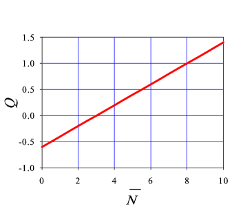
Figure 2: Plot of the Mandel $Q$ parameter for the optimum distribution $p_{N}$ obtained numerically from (Maximally polarized states for quantum light fields) in terms of the average number of photons $\bar{N}$ of the state.

In Fig. 3 we have plotted the optimum distribution $p_{N}$ for different integer values of $\bar{N}$ running from 1 to 9. The truncation value has been chosen to be 25 in all the cases, although it is sufficient to ensure, for each value of $\bar{N}$, that $p_{N}\simeq 0$ for $N>D$. Three distinctive features can be immediately discerned: the solutions are symmetric around $\bar{N}$, they are parabolic, and extend in a range from 0 to $2\bar{N}$. The two first facts are in agreement with the symmetry properties of the original problem (Maximally polarized states for quantum light fields). The third one means a variance that scales as $\bar{N}^{2}$, at difference of what happens for standard coherent optical processes presenting a variance linear with $\bar{N}$ (as for, e.g., in Poissonian or Gaussian statistics). In other words, the optimum states are extremely noisy and fluctuating. When $\bar{N}$ is not integer (or semi-integer), one can appreciate a small asymmetry that is less and less noticeable as $\bar{N}$ increases.

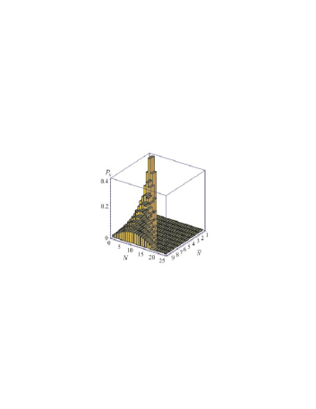
Figure 3: Optimum distribution $p_{N}$ plotted as a function of the average number of photons $\bar{N}$ and $N$. We have taken $\bar{N}$ to be a integer running from 1 to 9 and the dimension of the space $D=25$.

We conclude that we can take the dimension $D$ to be $2\bar{N}$. Given the very simple form of $H$ and $A$, we can express the final solution (15) in a closed analytic form:

$$p_{N}=3\frac{(\bar{N}+1)^{2}-(N-\bar{N})^{2}}{(2\bar{N}+1)(\bar{N}+1)(2\bar{N}+3)}\simeq\frac{3}{2\bar{N}}\left(\frac{N}{\bar{N}}-\frac{1}{2}\frac{N^{2}}{\bar{N}^{2}}\right)\,,$$ (17)

which is properly normalized and shows all the aforementioned characteristics, with a maximum value of $p_{\bar{N}}\simeq 3/(4\bar{N})$. If we use $x=N/(2\bar{N})$, which can be considered as a quasicontinuous variable $0\leq x\leq 1$, we can convert (17) in $p(x)=(3/\bar{N})\ x(1-x)$, which is the Beta distribution of parameters $(2,2)$ Evans2000 . For the solution (17), the corresponding degree of polarization is

$$\mathbb{P}_{\mathrm{opt}}=1-\frac{3}{(2\bar{N}+1)(2\bar{N}+3)}\sim 1-\frac{3}{4\bar{N}^{2}}\,.$$ (18)

This provides a full characterization of the optimum states we were looking for. However, their physical implementation stands as a serious problem. The crucial issue for the scaling in (18) is the fact that distribution variance is proportional to $\bar{N}^{2}$. It turns out that, for the discrete uniparametric distributions usually encountered in physics, this is distinctive of the thermal (or geometric) distribution

$$p_{N}=\frac{1}{\bar{N}+1}\left(\frac{\bar{N}}{\bar{N}+1}\right)^{N}\,.$$ (19)

But this is the photon statistics associated with the states

$$|\xi\rangle=\frac{1}{\cosh\xi}\,\sum_{n=0}^{\infty}\tanh^{n}\xi\;|n\rangle_{H}\otimes|n\rangle_{V}\,,$$ (20)

which are the twin beams generated in an optical parametric amplifier with a vacuum-state input, with $\bar{N}=2\sinh^{2}\xi$. The distribution (19) presents a skewness absent in the exact solution (17), but a calculation of the state degree of polarization gives

$$\mathbb{P}_{\xi}\simeq 1-\frac{\ln(\bar{N}/2)}{\bar{N}^{2}}\,.$$ (21)

Apparently, this is different from (18), but as soon as $\bar{N}\gg 1$ they both approach unity in essentially the same way, which means that the (maximally entangled) squeezed vacuum (20) is very close to optimum when $\bar{N}\gg 1$. In fact, one can calculate the degree of polarization for (20) using other metrics than the Hilbert-Schmidt. For example, if one employs the Bures (or fidelity) distance, a simple exercise shows that $\mathbb{P}^{\mathrm{Bures}}_{\xi}=1-1/\bar{N}^{2}$, confirming again the fundamental scaling $\bar{N}^{-2}$.

Before ending, two important remarks seem in order. First, we observe that in classical optics fully polarized fields have a perfectly defined relative phase between $H$- and $V$-polarized modes Bro98 . Such a relation does not necessarily hold in the quantum domain: while the quadrature coherent states (8) have a sharp relative phase, the twin-photon beams (20) have an almost random relative phase. Second, the maximally polarized states we have found have a highly nonclassical behavior, even in the limit $\bar{N}\gg 1$, which makes the classical limit of these polarized states a touchy business.

We thank A. Felipe and M. Curty for helpful discussions. This work was supported by the Swedish Foundation for International Cooperation in Research and Higher Education (STINT), the Swedish Foundation for Strategic Research (SSF), the Swedish Research Council (VR), the CONACyT grant PROMEP/103.5/04/1911, and the Spanish Research Project FIS2005-0671.

References

- (1) M. Hillery, Phys. Rev. A 35, 725 (1987); 39, 2994 (1989); V. V. Dodonov, O. V. Man’ko, V. I. Man’ko and A. Wünsche, J. Mod. Opt. 47, 633 (2000); P. Marian, T. A. Marian, and H. Scutaru, Phys. Rev. A 69, 022104 (2004).
- (2) V. Vedral, M. B. Plenio, M. A. Rippin, and P. L. Knight, Phys. Rev. Lett. 78, 2275 (1997); V. Vedral and M. B. Plenio, Phys. Rev. A 57, 1619 (1998).
- (3) C. A. Fuchs and C. M. Caves, Phys. Rev. Lett. 73, 3047 (1994); B. Schumacher, Phys. Rev. A 51, 2738 (1995); Č. Brukner and A. Zeilinger, Phys. Rev. Lett. 83, 3354 (1999); T. Rudolph and B. C. Sanders, Phys. Rev. Lett. 87, 077903 (2001); A. Gilchrist, N. K. Langford, and M. A. Nielsen, Phys. Rev. A 71, 062310 (2005).
- (4) H. Maassen and J. B. M. Uffink, Phys. Rev. Lett. 60, 1103 (1988); A. Anderson and J. J. Halliwell, Phys. Rev. D 48, 2753 (1993); S. Gnutzmann and K. Życzkowski, J. Phys. A 34, 10123 (2001).
- (5) T. Saastamoinen and J. Tervo, J. Mod. Opt. 51, 2039 (2004); A. Luis, Phys. Rev. A 66, 013806 (2002); A. B. Klimov, L. L. Sánchez-Soto, E. C. Yustas, J. Söderholm, and G. Björk, Phys. Rev. 72, 033813 (2005)
- (6) W. K.Wootters, Phys. Rev. D 23, 357 (1981).
- (7) J. M. Jauch and F. Rohrlich, The Theory of Photons and Electrons (Addison, Reading MA, 1959); A. Luis and L. L. Sánchez-Soto, Prog. Opt. 41, 421 (2000).
- (8) D. N. Klyshko, Uspehi. Fiz. Nauk 166, 613 (1996).
- (9) H. Prakash and N. Chandra, Phys. Rev. A 4, 796 (1971); G. S. Agarwal, Lett. Nuovo Cimento 1, 53 (1971); J. Lehner, U. Leonhardt, and H. Paul, Phys. Rev. A 53, 2727 (1996); J. Söderholm, G. Björk, and A. Trifonov, Opt. Spectrosc. (USSR), 91, 540 (2001).
- (10) A. M. Perelomov, Generalized Coherent States and Their Applications (Springer, Berlin, 1986).
- (11) S. Boyd and L. Vandenberghe, Convex Optimization (Cambridge U. Press, Cambridge, 2004).
- (12) L. Mandel and E. Wolf, Coherence and Quantum Optics (Cambridge U. Press, Cambridge, 1995).
- (13) M. Evans, N. Hastings, and B. Peacock, Statistical Distributions (Wiley, New York, 2000), 3 edn.
- (14) C. Brosseau, Fundamentals of Polarized Light: A Statistical Optics Approach (Wiley, New York, 1998).