Cavity QED determination of atomic number statistics in optical lattices

Abstract

We study the reflection of two counter-propagating modes of the light field in a ring resonator by ultracold atoms either in the Mott insulator state or in the superfluid state of an optical lattice. We obtain exact numerical results for a simple two-well model and carry out statistical calculations appropriate for the full lattice case. We find that the dynamics of the reflected light strongly depends on both the lattice spacing and the state of the matter-wave field. Depending on the lattice spacing, the light field is sensitive to various density-density correlation functions of the atoms. The light field and the atoms become strongly entangled if the latter are in a superfluid state, in which case the photon statistics typically exhibit complicated multimodal structures.

I Introduction

The study of ultracold atoms in optical lattices has been a very active field of research both experimentally and theoretically in recent years. One motivation to study these systems is that they provide clean realizations of important models of condensed matter physics lew such as the Bose-Hubbard and Fermi-Hubbard models Jaksch et al. (1998); Jaksch and Zoller (2005), spin systems J. J. Garcia-Ripoll et al. (2004) and the Anderson lattice model Miyakawa and Meystre (2006). A particularly well-known example is the prediction Jaksch et al. (1998) and observation of the Mott-insulator to superfluid transition Greiner et al. (2002a, b) in trapped Rubidium atoms. An important advantage of ultracold atoms over conventional solid-state systems is that they offer an exquisite degree of control over system parameters such as interaction strengths, densities and tunneling rates. Ultracold atomic systems are also very versatile in that the atoms involved can be either fermionic or bosonic, and can be associated into molecules of either statistics Rom et al. (2004); T. Stöferle et al. (2006); Thalhammer et al. (2006); Jaksch et al. (2002). Furthermore the dimensionality of the systems can be tuned from three to two and one-dimensional. Important other potential applications of ultracold atoms in lattices include quantum information Jaksch et al. (1999); Mandel et al. (2003) and improved atomic clocks Takamoto et al. (2005).

The ability to characterize the many-particle state of atomic fields is an important ingredient of many of these studies. While a full characterization of the field would ideally be desirable, a great deal can already be learned from the atomic density fluctuations at each lattice site and from the intersite density correlations. The counting statistics of atoms in an optical lattice have previously been studied by using spin changing collisions Gerbier et al. (2006), atomic interferences in free expansion Roberts and Burnett (2003) and the conversion of atoms into molecules via photoassociation Ryu et al. (2005) or Feshbach resonances T. Stöferle et al. (2006). The main goal of this paper is to propose and analyze an alternative cavity-QED based method to measure these properties.

Our proposed scheme is an extension to trapped ultracold atoms of the familiar diffraction technique used to probe order in crystalline structures. One important new aspect is that since we wish to measure the quantum fluctuations of the atomic density we cannot simply use classical radiation, which only provides information on some average of the atomic occupation numbers. Instead, we exploit the quantum nature of the light field and the fact that it can become entangled with the atoms to probe the number statistics of the matter-wave field. It is for this reason that a cavity-QED geometry is particularly attractive: as is well known, high-$Q$ optical cavities can significantly isolate the system from its environment, thus strongly reducing decoherence and ensuring that the light field remains quantum mechanical for the duration of the experiment.

More specifically, we consider two counter-propagating field modes in a high-$Q$ ring cavity, coupled via Bragg scattering off the atoms trapped in an optical lattice. If one of the counter-propagating modes is initially in vacuum, this is analogous to a quantum version of the Bragg reflection of X-rays by a crystal.

The remainder of this article is organized as follows: Section II describes our model and presents several general results of importance for the following analysis. In particular, it shows that the dynamics of the light field strongly depends on the manybody state of the atomic field as well as on the lattice spacing. Section III presents a series of results for the case of a simple two-well system, analyzing the properties of the Bragg-reflected light field for atoms in a Mott insulator state and for a superfluid described both in terms of a number-conserving state and of a mean-field coherent state. In particular, we find that these two descriptions lead to major differences in the properties of the scattered light. Section IV then turns to the case of a large lattice. Finally, section V is a conclusion and outlook.

II Model

We consider a sample of bosonic two-level atoms with transition frequency $\omega_{a}$ trapped in the lowest Bloch band of a one-dimensional optical lattice with $M$ lattice sites and a lattice spacing $d$, see Fig. 1. We assume for simplicity that the effects of tunneling and collisions are fully accounted for by the initial state of the matter-wave field, and neglect them during the subsequent scattering of the weak quantized probe fields, taken to be two counter-propagating (plane-wave) modes of a ring cavity with mode functions $\mathcal{E}_{\pm k}(z)$, wave-vectors $\pm k$ and frequency $\omega_{k}$. We further assume that these fields are far detuned from the atomic transition, $|\Delta|\equiv|\omega_{k}-\omega_{a}|\gg\gamma,\Omega_{R}$, with $\gamma$ the atomic linewidth and $\Omega_{R}$ the vacuum Rabi frequency, so that the excited electronic state of the two-level atoms can be adiabatically eliminated.

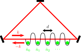
Figure 1: (Color online) Atoms trapped in an optical lattice with lattice constant $d$ in a ring resonator and interacting with two counter-propagating modes with wave vectors $\pm k$.

Expanding the field operators for the atomic excited state $\hat{\psi}^{(e)}(z)$ and ground state $\hat{\psi}^{(g)}(z)$ in the Wannier basis of the lowest Bloch band as

$$\hat{\psi}^{(e,g)}(z)=\sum_{m=0}^{M-1}\psi_{m}^{(e,g)}(z)\hat{c}_{m}^{(e,g)},$$

where $\hat{c}_{m}^{(e)}$ and $\hat{c}_{m}^{(g)}$ are the bosonic annihilation operators for an atom in the excited and ground state at lattice site $m$ and $\psi_{m}^{(e)}$ and $\psi_{m}^{(g)}$ the corresponding wave functions, this system is described by the effective Hamiltonian

$$\hat{H} = \hbar g[\hat{N}(0)(\hat{a}_{k}^{\dagger}\hat{a}_{k}+\hat{a}_{-k}^{\dagger}\hat{a}_{-k})$$ (1)

$$+\hat{N}(d)\hat{a}_{-k}^{\dagger}\hat{a}_{k}+\hat{N}(-d)\hat{a}_{k}^{\dagger}\hat{a}_{-k}],$$

where we have neglected collisions and tunneling, as already discussed, and also ignore all loss processes. In this expression

$$\hat{N}(d)=\sum_{m=0}^{M-1}e^{2imkd}\hat{c}_{m}^{(g)\dagger}\hat{c}_{m}^{(g)}$$ (2)

and the coupling frequency is

$$g=\frac{2\wp^{2}}{\Delta\hbar^{2}}\left|\int dz\mathcal{E}_{\pm k}(z)\psi_{0}^{(e)*}(z)\psi_{0}^{(g)}(z)\right|^{2},$$ (3)

with $\wp$ the dipole matrix element of the atomic transition. Since only the ground electronic state is relevant in this model, we drop the superscript $(g)$ in the following for notational clarity.

Our proposed detection scheme relies crucially on the observation of the coherent dynamics resulting from the Hamiltonian (1), hence it is important that the associated characteristic time scales are significantly faster than than those associated with losses and with the atomic motion in the lattice. To illustrate that this is within current experimental reach, we consider explicitly the experimental parameters of Klinner et. al. Klinner et al. (2006). Assuming that the atoms are confined to much less than an optical wavelength at the antinodes of the lattice potential, we can approximate the coupling constant between the cavity modes and a single atom as

$$g\approx\frac{\wp^{2}\omega_{k}}{\Delta\hbar\epsilon_{0}V},$$

where $V$ is the mode volume of the cavity and $\wp\approx 2.3\times 10^{-29}$ Cm is the relevant dipole matrix element for the $D_{2}$ line of ⁸⁵Rb. For a detuning of $\Delta=-1$ GHz from that transition, a cavity length of $0.1$ m, and a mode waist of $100\;\mu$m we find $g\approx 50$ s^-1.

As we show later on, the fluctuations of the operator $\hat{N}(d)$ are central in the determination of the spectral properties of $\hat{G}$. As these typically scale like the square root of the total number of atoms we find that for a sample of $10^{6}$ atoms the relevant frequencies for the coherent evolution are of the order of 50 kHz. Such frequencies are several times larger than the decay rate of state-of-the-art optical cavities with large mode volume, 17 kHz in the experiments of Klinneris et. al. The spontaneous emission from the atomic excited state is negligible at this detuning. Indeed, the fact that in the experiment of Klinner a splitting of the normal modes has been observed is direct experimental evidence that the coherent dynamics can be made dominant over the losses.

Turning now to the characteristic time scales for the center-of-mass atomic dynamics, specifically the interwell tunneling rate and the two-body collision rate, they can be controlled with high accuracy, respectively through the depth of the lattice potential and via a magnetic Feshbach resonance. It is therefore possible to operate under experimental conditions such that both are much smaller than the coupling strength between atoms and light. This justifies “freezing” the atomic dynamics resulting from tunneling and collisions once the probe fields are turned on.

It is well known that, depending upon the ratio between tunneling and two-body collisions, bosonic atoms in an optical lattice can undergo a transition from a superfluid to a Mott insulator state. With this in mind, we consider initial atomic states that correspond to these two extreme situations, specifically: (a) a Mott insulator state with a well-defined atom number in each well, (b) a state where each well is in a coherent state, a mean-field approximation of the superfluid state, and (c) a more realistic description of atoms in the superfluid state with a fixed total number of atoms $N$. These three states are given explicitly by

$$|\psi_{\rm Mott}\rangle=|n_{0},n_{1},\ldots,n_{M-1}\rangle,$$ (4)

$$|\psi_{\rm SF1}\rangle=|\alpha_{0},\alpha_{1},\ldots,\alpha_{M-1}\rangle,$$ (5)

where $|\alpha_{m}|^{2}$ is the mean number of atoms in well $m$, and

$$|\psi_{\rm SF2}\rangle=\mathcal{N}^{-1}\left(\sum_{m=0}^{M-1}\ {\hat{c}}_{m}^{\dagger}\right)^{N}|0\rangle,$$ (6)

where $\mathcal{N}=\sqrt{N!M^{N}}$ is a normalization constant.

We further assume for simplicity that the mode propagating in the $-k$ direction along the ring is initially in a vacuum while the other mode is in a Fock state with $n_{\rm tot}$ photons. Our results are qualitatively independent of the exact state of the light field, but we will point out the modifications brought about by a coherent state instead of a number state when appropriate.

The intensities of the two counter-propagating modes, $\langle\hat{a}_{k}^{\dagger}\hat{a}_{k}\rangle$ and $\langle\hat{a}_{-k}^{\dagger}\hat{a}_{-k}\rangle$, are easily obtained from the solution of the Heisenberg equations of motion for ${\hat{a}}_{\pm k}(t)$,

$$\left[\begin{array}[]{c}\hat{a}_{-k}(t)\\ \hat{a}_{k}(t)\end{array}\right]=e^{-ig\hat{N}(0)t}\left[\begin{array}[]{cc}\cos\hat{G}(d)t&-i\hat{Q}(d)\sin\hat{G}(d)t\\ -i\hat{Q}^{\dagger}(d)\sin\hat{G}(d)t&\cos\hat{G}(d)t\end{array}\right]\left[\begin{array}[]{c}\hat{a}_{-k}(0)\\ \hat{a}_{k}(0)\end{array}\right],$$ (7)

where

$$\hat{Q}(d)=\frac{\hat{N}(d)}{\sqrt{\hat{N}(d)\hat{N}(-d)}}$$ (8)

is unitary and we have introduced the operator

$$\hat{G}(d)=g\sqrt{\hat{N}(d)\hat{N}(-d)}$$ (9)

describing the coupling between the two modes. The closed form solution (7) follows from the observation that in the absence of tunneling the optical field only couples to conserved quantities of the atomic field. Note however that the number statistics of the atoms at each site is conserved for many cases of practical interest even in the presence of tunneling. This is for instance the case for the ground state of the Bose-Hubbard model. Our results are valid for such cases as well.

Expanding the atomic states in the number states basis $|n_{0},n_{1},\ldots,n_{M-1}\rangle$, where the operators $\hat{G}$ and $\hat{Q}$ are diagonal, we then find for the intensity of the Bragg-reflected field

$$\frac{\langle\hat{n}_{-k}(t)\rangle}{n_{\rm tot}} = \frac{1}{2}-\frac{1}{2}\sum_{n_{0},n_{1},\ldots,n_{M-1}}P_{n_{0},n_{1},\ldots,n_{M-1}}$$ (10)

$$\times \cos 2\omega(n_{0},n_{1},\ldots,n_{M-1})t,$$

where $P_{n_{0},n_{1},\ldots,n_{M-1}}$ is the probability to find $n_{m}$ atoms in the $m^{\rm th}$ well and $\omega(n_{0},n_{1},\ldots,n_{M-1})$ is the corresponding eigenvalue of $\hat{G}$.

As we see in the following sections, this expression accounts implicitly for the well-known property that Bragg scattering depends strongly on the well separation $d$. In particular, the light scattered from neighboring wells interferes either constructively or destructively for well separations equal to $\lambda/2$ or $\lambda/4$, respectively, two situations relatively easy to realize experimentally.

III Double-well potential

Before considering the situation of a general optical lattice, we discuss the simpler case of a double-well potential, where explicit analytical results are readily obtained. Despite its simplicity, this case already exhibits many of the properties of the full $M$-site lattice and hence provides valuable intuition for its understanding. We first discuss the Bragg-reflected intensity for well separations $d=\lambda/2$ and $d=\lambda/4$, and then turn to an arbitrary well separation and to the analysis of the photon statistics.

III.1 Reflected intensity

III.1.1 Well separation $d=\lambda/2$

From Eq. (10), most properties of the reflected intensity can be understood from an analysis of the eigenvalues of the operator $\hat{G}(d)$ describing the coupling between the forward- and backward-propagating light fields. For $d=\lambda/2$ we find from the definition (2) of ${\hat{N}}(d)$ that

$$\hat{G}(\lambda/2)=g(\hat{n}_{0}+\hat{n}_{1}),$$

indicating that the intensity of the Bragg-scattered light is only sensitive to the total number of atoms $N$, a signature of the constructive interference of the fields reflected off the two wells. Specifically,

$$\frac{\langle\hat{n}_{-k}(t)\rangle}{n_{\rm tot}}=\sum_{N=0}^{\infty}P_{N}\sin^{2}gNt$$ (11)

where $P_{N}$ is the probability that the total atom number in the two wells is $N$.

Both the Fock state $|\psi_{\rm Mott}\rangle$ and superfluid state $|\psi_{\rm SF2}\rangle$ have a well defined total number of atoms so that the light field simply undergoes harmonic oscillations between the $+k$ and $-k$ directions. These two situations are illustrated in the upper and lower parts of Fig. 2.

Figure 2: Reflected intensities $\langle\hat{n}_{-k}(t)\rangle$ for well separation $d=\lambda/2$ and for atoms (a) in a Fock state $|\psi_{\rm Mott}\rangle$, (b) in a superfluid state in mean field approximation $|\psi_{\rm SF1}\rangle$ and (c) in the number-conserving superfluid state $|\psi_{\rm SF2}\rangle$. The mean number of atoms in each well is nine in all three cases.

In contrast, if the atomic field is described by coherent states for each well, the total number of atoms is uncertain and consequently the reflected intensity is comprised of oscillations at the eigenfrequencies associated to all possible combinations of atom numbers, leading to collapses and revivals similar to those familiar from the two-photon Jaynes-Cummings model Buck and Sukamar (1981); Sukamar and Buck (1981), see the middle curve in Fig. 2. The Bragg-reflected intensity periodically collapses and revives after characteristic times

$$T^{\lambda/2,\rm SF1}_{\rm collapse}=\frac{1}{2g\Delta(\hat{n}_{0}+\hat{n}_{1})}=\frac{1}{2g\sqrt{\langle\hat{n}_{0}\rangle+\langle\hat{n}_{1}\rangle}},$$ (12)

and

$$T_{\rm revival}=\pi/g,$$ (13)

where $\Delta(\hat{n}_{0}+\hat{n}_{1})=\sqrt{\langle(\hat{n}_{0}+\hat{n}_{1})^{2}\rangle-\langle\hat{n}_{0}+\hat{n}_{1}\rangle^{2}}$ is the standard deviation of the total number of atoms. Equation (12) is important in that it indicates that the intensity of Bragg-scattered light is indeed sensitive to fluctuations in the atom number. As such, it offers a clear signature to distinguish the mean-field description from the number-conserving description of the atomic superfluid state.

III.1.2 Well separation $d=\lambda/4$

The light reflected from the two wells is now $\pi$ out of phase and hence interferes destructively. Mathematically, this is reflected by the coupling between the two counter-propagating modes being now proportional to the difference between the atom numbers in the two wells,

$$\hat{G}(\lambda/4)=g|\hat{n}_{0}-\hat{n}_{1}|,$$

so that the intensity of the backscattered light field is given by

$$\frac{\langle\hat{n}_{-k}(t)\rangle}{n_{\rm tot}}=\sum_{|\Delta N|=0}^{\infty}P_{|\Delta N|}\sin^{2}g|\Delta N|t,$$ (14)

where $P_{|\Delta N|}$ is the probability that the atomic population difference between the two wells is $\Delta N$ or $-\Delta N$.

If the atomic fields in both wells are in Fock states, the sum in Eq. (14) reduces to just one term and the light intensity undergoes sinusoidal oscillations at frequency $g|n_{0}-n_{1}|$. If the atom numbers are equal the two optical modes become decoupled, see Fig. 3(a).

Figure 3: Reflected intensities $\langle\hat{n}_{-k}(t)\rangle$ for well separation $d=\lambda/4$ and for the atoms (a) in Fock states with equal atom numbers, (b) in coherent states of equal mean atom number and (c) in the number-conserving superfluid state. The mean number of atoms in each well is nine in all cases. In (c) the solid line is for $N=18$ and the dashed line is for $N=17$.

If each well is in a coherent state, on the other hand, the number difference is not known with certainty and accordingly the oscillations of the intensities of the two modes contain frequency components corresponding to all possible number differences. In the case of equal mean atomic numbers in the two wells the reflected intensity rises to half the initial intensity of the forward-propagating field, remains constant at this value and drops to zero at time $T_{\rm revival}$. The dips in the reflected intensity can be thought of as ‘remnants’ of the collapse and revival features exhibited by the $d=\lambda/2$ case. Similarly to that case the half-width of the dips is determined by the uncertainty in the atom number difference, which is half of the uncertainty in the total number of atoms , so that the initial rise time is given by $T^{\lambda/4,\rm SF1}_{\rm collapse}=2T^{\lambda/2,\rm SF1}_{\rm collapse}=1/g\sqrt{\langle\hat{n}_{0}\rangle+\langle\hat{n}_{1}\rangle}$.

Finally, for atoms in the number-conserving superfluid state $|\psi_{\rm SF2}\rangle$, odd differences in atomic numbers are impossible for an even total number of atoms, hence all possible oscillation frequencies differ by at least $2g$ (or $4g$ for the oscillations of the field intensities). For an even total number of atoms the revival time is cut in half, see Fig. 3(c). For odd numbers of atoms the reflected intensity is equal to $n_{\rm tot}$ at times $t=\pi/2g,\;3\pi/2g,\ldots$ Apart from these times the reflected intensity behaves very similar to the coherent state case. The collapse time is $T^{\lambda/4,\rm SF2}_{\rm collapse}=2T^{\lambda/2,\rm SF1}_{\rm collapse}$.

III.1.3 Arbitrary well separation

The expressions (11) and (14) for the backscattered photon numbers in the two cases considered so far indicate that the marginal probability distributions $P_{N}$ and $P_{|\Delta N|}$ can be directly determined from the reflected intensity by means of Fourier transforms. Unfortunately, the complete number statistics $P_{n_{0},n_{1}}$ for $n_{0}$ atoms in the first well and $n_{1}$ atoms in the second well cannot be reconstructed from these marginals.

The dynamics of the two optical modes becomes more involved for arbitrary separations, as the eigenvalues of the operator $\hat{G}$ are no longer integer multiples of $g$ but in general irrational numbers that depend on the occupation numbers $\hat{n}_{0}$ and $\hat{n}_{1}$ in a nontrivial manner. One consequence is that the perfect recurrences observed for $d=\lambda/2$ and $d=\lambda/4$ no longer occur and the dynamics of the backscattered intensity is typically non-periodic.

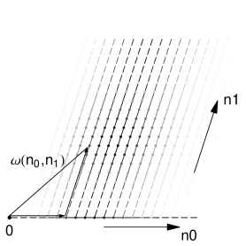
Figure 4: Construction of the eigenvalues of $\hat{G}$ for $d=\lambda/10$ and probability of occurrence of each frequency for the two wells in coherent states with coherent amplitudes $\alpha_{1}=\alpha_{2}=3$.

Figure 5: Backscattered intensity for atoms in state $|\psi_{\rm SF1}\rangle$ with nine atoms in each well on average and a well separation $d=\lambda/10$.

The backscattered intensity is determined by the spectral properties of the operator $\hat{G}$ as we have seen, and these can be understood by means of a simple geometric construction: For a number state with $n_{0}$ atoms in the first well and $n_{1}$ atoms in the second well the eigenvalue of $\hat{G}$ is given by the hypothenuse of the triangle obtained by drawing a straight line of length $gn_{0}$ and then continuing with another straight line of length $gn_{1}$ at an angle $2kd$ with respect to the first line. This construction is shown in Fig. 4, which also illustrates the probability of each frequency occurring if each well is in a coherent state with coherent amplitude $\alpha_{0}=\alpha_{1}=3$. The dots along the $n_{0}$ line are drawn in shades of gray with darker shades being more likely and lighter shades being less likely. The $n_{1}$ lines originating from each dot are drawn with the same convention, and the probability for a given combination of $n_{0}$ and $n_{1}$, obtained by multiplying the probabilities for $n_{0}$ and $n_{1}$, is again shown in gray scale. Hence the most likely eigenfrequencies and the spread in frequencies can be read off as the distances of the final dots from the origin. A typical example of Bragg-reflected intensity is shown in Fig. 5. This example is for nine atoms per well in the coherent state $|\psi_{\rm SF1}\rangle$ and a well separation $d=\lambda/10$.

Figure 6 shows the spectrum of $\hat{G}$ as a function of $d$ for state $|\psi_{\rm SF1}\rangle$ with $\alpha_{0}=\alpha_{1}=3$. Each frequency is again weighted with its likelihood, and the eigenfrequencies have been collected in bins of the size of the pixels in the figure. The special cases of $d=\lambda/2$ and $d=\lambda/4$ are easily recognized, as for those well separations only integer multiples of $g$ can occur. For general well separations, the spectra lack any obvious structure.

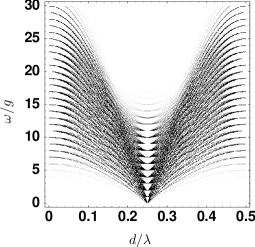
Figure 6: Spectrum of $\hat{G}$ as a function of $d$. The darkness of each eigenfrequency corresponds to its likelihood. In this example both wells are in a coherent state with an average of 9 atoms per well.

The number-conserving superfluid state $|\psi_{\rm SF2}\rangle$ corresponds roughly to a “diagonal cut” through the construction in Fig. 4 such that $n_{0}$ decreases by one if $n_{1}$ is increased by one. Accordingly there are now much fewer possible frequencies as can be seen in Fig. 7. Furthermore, the width of the frequency distribution is no longer independent of $d$. We have $\Delta|\hat{n}_{0}-\hat{n}_{1}|=\sqrt{\frac{N}{2}(1-\cos 2kd)}$ .

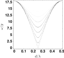
Figure 7: Spectrum of $\hat{G}$ as a function of $d$ for atoms in state $|\psi_{\rm SF2}\rangle$ with 18 atoms.

III.2 Photon number statistics

A major advantage of the two-well case over the full lattice case is that we can easily solve the Schrödinger equation for the coupled atom-cavity system numerically. This integration is greatly facilitated by the conservation of the number of atoms in each well and the total number of photons, which we exploit by integrating in the invariant subspaces of constant $\hat{n}_{0}$, $\hat{n}_{1}$ and $\hat{n}_{k}+\hat{n}_{-k}$. From the full solution we can gain more detailed information about the dynamics of the photons than the average reflected intensity considered so far.

Here we consider the number statistics of the Bragg-reflected photons,

$$P_{n_{-k}}=\langle|n_{-k}\rangle\langle n_{-k}|\rangle.$$ (15)

The calculation of $P_{n_{-k}}$ involves a trace over the well occupation numbers. As a consequence the number statistics is, in complete analogy to the reflected intensity in Eq. (10), the sum of the number statistics $P_{n_{-k}}^{(n_{0},n_{1})}$ for each set of occupation numbers $(n_{0},n_{1})$, each weighted with its probability of occurring in the atomic state,

$$P_{n_{-k}}=\sum_{n_{0},n_{1}}P_{n_{0},n_{1}}P_{n_{-k}}^{(n_{0},n_{1})}.$$

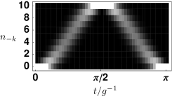
Figure 8: Photon number statistics $P_{n_{-k}}(t)$ for each well in a Fock state with $n_{0}=9$ and $n_{1}=10$ atoms, a well separation of $d=\lambda/4$ and 10 photons initially in the $+k$ direction. Lighter shades of grey correspond to higher probabilities.

Figure 8 shows one of the building blocks $P_{n_{-k}}^{(n_{0},n_{1})}(t)$ for well occupation numbers $n_{0}=10$ and $n_{1}=9$ with $d=\lambda/4$. In this case the two counter-propagating modes are linearly coupled to each other, with coupling frequency $g|n_{0}-n_{1}|$. Figure 9 shows the number statistics for atoms in state $|\psi_{\rm SF2}\rangle$.

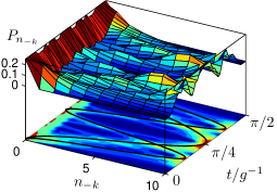
Figure 9: (Color online) Photon number statistics for atoms in state $|\psi_{\rm SF2}\rangle$ for $N=18$ atoms and a well separation $d=\lambda/4$. Also indicated are the elementary sinusoidal oscillations corresponding to number differences one and two.

This example is representative of the typical situation, with non-trivial photon statistics and ‘complicated’ dynamics of the light field that cannot be adequately described by means of the reflected intensity only. As the elementary probability wavepackets $P_{n_{-k}}^{(n_{0},n_{1})}(t)$ dephase with respect to each other the photon statistics evolves through complex patterns, with a large uncertainty of the photon number. The reflected light intensity exhibits large fluctuations the description of which requires all moments of the intensity up to order $n_{\rm tot}$.

There are however special times when several of the elementary photon statistics building blocks add up to yield peaks at specific photon numbers. Prominent such times are $t=\pi/2g^{-1}$ and $t=\pi/4g^{-1}$ for $d=\lambda/4$. At these times all odd frequency components (i.e. odd number differences) lead to $\hat{n}_{-k}=n_{\rm tot}$ while all even number differences lead to $\hat{n}_{-k}=0$. This is illustrated in Fig. 10 for the atomic state $|\psi_{\rm SF1}\rangle$. For the fairly large mean number of atoms per well considered in that example the probabilities for even and odd frequencies are approximately equal so that the probabilities to find all photons reflected or no reflection at all are also nearly equal. For atoms in state $|\psi_{\rm SF2}\rangle$ the photon statistics at time $t=\pi/4g^{-1}$ look very similar to Fig. 10(b).

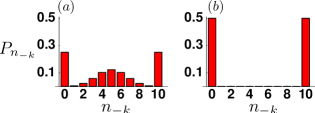
Figure 10: (Color online) Photon number statistics at times (a) $t=\pi/4g^{-1}$ and (b) $t=\pi/2g^{-1}$ for atoms in state $|\psi_{\rm SF1}\rangle$ with average atom numbers $n_{0}=n_{1}=9$ for well separation $d=\lambda/4$.

It is important to emphasize that the light field does not evolve into a ‘NOON’ state $(|n_{\rm tot},0\rangle+|0,n_{\rm tot}\rangle)/\sqrt{2}$, which would show the same behavior. Rather, the light field is entangled with the atoms in the Schrödinger cat state

$$|\psi(t=\pi/2g)\rangle=|\psi_{\rm SC}\rangle$$

$$= \frac{1}{2}|n_{\rm tot},0\rangle\left[|\alpha_{0},(-1)^{n_{\rm tot}}\alpha_{1}\rangle+|-\alpha_{0},-(-1)^{n_{\rm tot}}\alpha_{1}\rangle\right]+\frac{(-i)^{n_{\rm tot}}}{2}|0,n_{\rm tot}\rangle\left[|\alpha_{0},(-1)^{n_{\rm tot}}\alpha_{1}\rangle-|-\alpha_{0},-(-1)^{n_{\rm tot}}\alpha_{1}\rangle\right]$$

which is reflected by the atomic $Q$-function in the first well,

$$Q(\alpha)=\langle\psi_{\rm SC}|\alpha\rangle\langle\alpha|\psi_{\rm SC}\rangle\\ =\frac{1}{2\pi}\left(e^{-|\alpha-\alpha_{0}|^{2}}+e^{-|\alpha+\alpha_{0}|^{2}}\right).$$

For $d=\lambda/2$ the number statistics looks qualitatively similar to the $\lambda/4$ case. The most likely frequencies are however typically higher because of the constructive interference of the light reflected off the two wells that leads to the coupling frequency being $g(\hat{n}_{0}+\hat{n}_{1})$.

In practice, Fock states are very hard to realize. Typically the $+k$ mode will start out in a superposition of states with different photon numbers such as a coherent state. As we have mentioned, this case is qualitatively similar to the Fock state case and here we would like to explain in more detail why this is so. Because the system Hamiltonian conserves the total number of photons $\hat{n}_{-k}+\hat{n}_{k}$, no interference between states with different total photon numbers can arise in any observable that preserves the total photon number as well. The reflected intensity and the photon number statistics are clearly observables of this type. For a general state the expectation value of these observables is the sum of the expectation values for the various photon numbers weighted with the probability of that photon number. The consequence is simply that one has additional fluctuations in the reflected intensity due to the uncertainty of the photon number in the initial state. Another way to see that the intensity behaves the same for all initial states of the $+k$ mode is to insert the formal solution for the modes of the light field Eq. (7) into the expectation value of the intensity. The terms containing operators of the $-k$ mode vanish and we end up with the expectation value of the intensity in the $+k$ mode at time $t=0$ multiplying the trace of the atomic operators over the atomic states.

IV Optical Lattice

IV.1 Well separation $d=\lambda/2$

This section extends the results of the double well analysis to the case of an optical lattice with a large number of wells. The case of a well separation $d=\lambda/2$ is again particularly simple since in that case $\hat{G}$ is simply proportional to the total number of atoms in the lattice,

$$\hat{G}=g\sum_{m}\hat{n}_{m}\equiv g\hat{N}.$$ (16)

Both the Fock state and the number-conserving superfluid state $|\psi_{\rm SF2}\rangle$ have a well-defined total number of atoms $N$, hence the intensity of the optical field undergoes simple sinusoidal oscillations at frequency $gN$ between the two counter-propagating modes.

The situation is more complicated in the mean-field description of the superfluid state, in which case the matter-wave field at each lattice site is in a coherent state with mean number of atoms $n_{m}=\langle\hat{N}\rangle/M$. In the limit of a large lattice, $M\gg 1$, the central limit theorem permits to approximate the probability distribution of the total number of atoms to an excellent degree as

$$P_{N}=\frac{1}{\sqrt{2\pi\langle\hat{N}\rangle}}\exp\left[{-\frac{(N-\langle\hat{N}\rangle)^{2}}{2\langle\hat{N}\rangle}}\right].$$ (17)

In the limit of large $\langle\hat{N}\rangle$ this distribution is sharply peaked at $\langle\hat{N}\rangle$ and the dynamics of the light is largely characterized by oscillations at frequency $g\langle\hat{N}\rangle$ between the two counter-propagating modes. However the finite variance of the total atomic number distribution results in a collapse of these oscillations on a time scale

$$T^{\lambda/2,{\rm SF1},latt.}_{\rm collapse}=\frac{1}{2g\sqrt{\langle\hat{N}\rangle}}.$$ (18)

The photons undergo roughly $2\sqrt{\langle\hat{N}\rangle}$ oscillations before this collapse. Note that since the allowed frequencies are discrete and integer multiples of $g$, the oscillations also show complete revivals, with a revival time given by Eq. (13).

IV.2 Well separation $d=\lambda/4$

The situation is markedly different for a well separation $d=\lambda/4$. In that case $\hat{G}$ is proportional to the difference in the total number of atoms trapped on even and odd lattice sites,

$$\hat{G}=g\left|\sum_{m\;{\rm even}}\hat{n}_{m}-\sum_{m\;{\rm odd}}\hat{n}_{m}\right|\equiv g|\hat{N}_{e}-\hat{N}_{o}|,$$ (19)

and the light field probes fluctuations in the occupation differences of neighboring sites. This is a useful property since fluctuations of this type, while being typically difficult to measure, can serve to distinguish various many-body quantum states such as the Mott insulator state and the superfluid state. Note that if all lattice sites are in Fock states with equal atomic population, then $\hat{G}$ vanishes identically for an even number of lattice sites and is very small when the number of lattice sites is odd. In typical experiments the atoms are also subject to a harmonic trap and the added trapping potential leads to shells with constant occupation number separated from each other by edges with a superfluid component. Equation (19) shows that the reflected light can serve as a good detector of these edges.

For the atoms in the mean-field superfluid state $|\psi_{\rm SF1}\rangle$ the coupling strength can again be analyzed using the central limit theorem. To this end we use the fact that $N_{e}$ and $-N_{o}$ are the sums of a large number of independent random variables with means $\langle\hat{N}\rangle/2$ and $-\langle\hat{N}\rangle/2$, respectively, and standard deviation $\sqrt{\langle\hat{N}\rangle/2}$. From the resulting Gaussian probability distributions for $N_{e}$ and $N_{o}$ we readily find the probability distribution for $N_{e}-N_{o}$ by using that the sum of two Gaussian random variables is again a Gaussian. For the intensity of the reflected light it is actually $|N_{e}-N_{o}|$ that is important, see Eq. (14). The probability distribution for this quantity is readily found from those for $N_{e,o}$ as

$$P_{|N_{e}-N_{o}|}=(2-\delta_{N_{e},N_{o}})\frac{1}{\sqrt{2\pi\langle\hat{N}\rangle}}\exp\left[{-\frac{(N_{e}-N_{o})^{2}}{2\langle\hat{N}\rangle}}\right],$$ (20)

where $\delta$ is the Kronecker delta.

The analysis of the state $|\psi_{\rm SF2}\rangle$ requires a bit more attention. Since $\hat{N}_{e}$ is the sum of many operators it is natural to assume that its distribution is Gaussian, and hence fully characterized by its mean $\langle\psi_{\rm SF2}|\hat{N}_{e}|\psi_{\rm SF2}\rangle=N/2$ and standard deviation $\Delta N_{e}=\sqrt{N}/2$. Since every choice of $N_{e}$ automatically determines $N_{o}=N-N_{e}$ the probability distribution for $|N_{e}-N_{o}|$ is

$$P_{|N_{e}-N_{o}|} = \delta_{N_{o}+N_{e},N}(2-\delta_{N_{e},N_{o}})$$ (21)

$$\times \frac{\sqrt{2}}{\sqrt{\pi N}}\exp\left[-\frac{(N_{e}-N_{o})^{2}}{2N}\right].$$

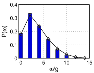
Figure 11: (Color online) Probability distribution of the coupling frequencies (eigenvalues of ${\hat{G}}$ for $d=\lambda/4$ with atoms in state $|\psi_{\rm SF2}\rangle$ for 10 lattice sites with 20 atoms. The bars are the exact probabilities determined numerically and the diamonds show the distribution obtained from Eq. (21). The line is an aid to the eye.

Figure 11 shows an example of the numerically obtained exact probability distribution and compares it to the approximate result of Eq. (21) for as few as 10 lattice sites and 20 atoms. Clearly, the two results already agree quite well even for these modest numbers, so that the expression (21) can be considered as essentially exact for the much larger numbers of lattice sites and atoms typically encountered in practice.

Note that if one assumes that the occupation numbers of the lattice sites contributing to $\hat{N}_{e}$ are independent when calculating the probability distribution for $N_{e}$ with the central limit theorem, one finds that the standard deviation of the resulting distribution is too large by a factor of $\sqrt{2}$. In this sense, fluctuations of the number difference between even and odd sites are suppressed in the state $|\psi_{\rm SF2}\rangle$.

IV.3 General well separation $d$

The calculation of the possible eigenvalues of $\hat{G}$ and their probabilities of occurring for the atomic states $|\psi_{\rm SF1}\rangle$ and $|\psi_{\rm SF2}\rangle$ by means of the central limit theorem can readily be extended to well separations $d=q\lambda/2p$, where $q$ and $p$ are integers. The lattice sites can be grouped into $p$ distinct classes according to the roots of unity $e^{2ikd}=e^{2i\pi l/p}$ with $l=0,1,\ldots,p-1$. The total number of atoms in each class ,

$$\hat{N}_{l}=\sum_{m=0}^{M/p-1}\hat{n}_{l+mp}$$

enters the frequency with the common coefficient $e^{2i\pi l/p}$ and each class comprises many lattice sites, so that the central limit theorem can be used to calculate the associated number distribution $P_{N_{l}}$ . The frequencies are then obtained as a function of the few macroscopic occupation numbers $\hat{N}_{l}$, which are independent to a good approximation. Thus the probabilities for the frequencies $\omega(N_{0},N_{1},\ldots,N_{p-1})=g|\sum_{l=0}^{p-1}N_{l}e^{2i\pi l/p}|$ are simply the product of the probabilities for each macroscopic occupation $P_{N_{l}}$. These probabilities can however not be written down in closed form, since the frequencies are no longer sums of Gaussian variables.

If $p$ is large or $d$ is an irrational fraction of $\lambda$, the behavior of the system becomes identical for atoms in states $|\psi_{\rm SF1}\rangle$ and $|\psi_{\rm SF2}\rangle$ in the limit of a large number of lattice sites. In this case we can think of $\hat{N}(d)$ as the result of a random walk of $M$ steps of average stride length $\langle N\rangle/M$ in the complex plane and the frequency is proportional to the distance from the origin to the final point. The distribution of possible frequencies $\omega$ becomes quasi-continuous with

$$P(\omega)=\frac{2\omega}{g^{2}\langle\hat{N}\rangle}\exp\left[-\frac{\omega^{2}}{g^{2}\langle\hat{N}\rangle}\right],$$ (22)

independently of whether the atoms are in state $|\psi_{\rm SF1}\rangle$ or $|\psi_{\rm SF2}\rangle$. This is illustrated in Fig. 12 for atoms in state $|\psi_{\rm SF1}\rangle$ and in Fig. 13 for atoms in state $|\psi_{\rm SF2}\rangle$. It is remarkable that the numerically obtained true frequency distribution is in a good agreement with the approximate Eq. (22) even for the low number of atoms and lattice sites considered here, and even more so, that this agreement is already obtained for $p=5$. As one might expect, we find much better agreement between the actual frequency distributions and Eq. (22) for the atom and site numbers of Figs. 12 and 13 if the lattice spacings correspond either to a larger $p$ or to irrational fractions of the optical wavelength, as is the case in the inset of Fig. 13, which is for $d=\sqrt{2}\lambda/10$.

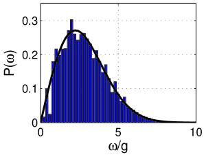
Figure 12: (Color online) Probability distribution of frequencies for atoms in the mean-field superfluid state $|\psi_{\rm SF1}\rangle$ with ten lattice sites and ten atoms for $d=\lambda/10$. The solid line is the distribution Eq. (22), and the histogram the result of an exact numerical diagonalization of ${\hat{G}}(d)$.

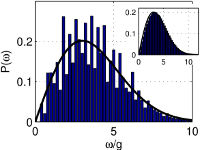
Figure 13: (Color online) Probability distribution of frequencies for atoms in the number-conserving superfluid state $|\psi_{\rm SF2}\rangle$ with ten lattice sites and 18 atoms for $d=\lambda/10$. The solid line is the distribution Eq. (22) and the histogram a result of the numerical diagonalization of ${\hat{G}}(d)$. The inset shows the same distribution for $d=\frac{\sqrt{2}}{10}\lambda$.

One can calculate the reflected intensity in closed form from the frequency distribution (22) by approximating the sum in Eq. (10) by an integral,

$$\frac{\langle\hat{n}_{-k}\rangle}{n_{\rm tot}} = \int_{0}^{\infty}d\omega P(\omega)\sin^{2}\omega t$$ (23)

$$= \frac{g\langle\hat{N}\rangle\sqrt{\pi}}{2\sqrt{M}}|t|e^{-\frac{g^{2}\langle\hat{N}\rangle^{2}t^{2}}{M}}{\rm erfi}\left(\frac{g\langle\hat{N}\rangle t}{\sqrt{M}}\right),$$

where ${\rm erfi}(x)=\frac{2}{i\sqrt{\pi}}\int_{0}^{ix}dze^{-z^{2}}$ is the complex error function. The intensity converges to $\langle\hat{n}_{-k}\rangle=n_{\rm tot}/2$ after a transient of duration $T_{\rm collapse}\approx\sqrt{M}/(g\langle\hat{N}\rangle)$.

lattice	atomic	$T_{\rm collapse}^{-1}$
spacing	state	2 wells	lattice
	$|\psi_{\rm Mott}\rangle$	$0$	$0$
$d=\frac{\lambda}{2}$	$|\psi_{\rm SF1}\rangle$	$2g\sqrt{\langle\hat{n}_{0}\rangle+\langle\hat{n}_{1}\rangle}$	$2g\sqrt{\langle\hat{N}\rangle}$
	$|\psi_{\rm SF2}\rangle$	$0$	$0$
	$|\psi_{\rm Mott}\rangle$	$0$	$0$
$d=\frac{\lambda}{4}$	$|\psi_{\rm SF1}\rangle$	$g\sqrt{\langle\hat{n}_{0}\rangle+\langle\hat{n}_{1}\rangle}$	$g\sqrt{1-2/\pi}\sqrt{\langle\hat{N}\rangle}$
	$|\psi_{\rm SF2}\rangle$	$g\sqrt{N}$	$g\sqrt{1-2/\pi}\sqrt{N}$
	$|\psi_{\rm Mott}\rangle$	$0$	$0$
general $d$	$|\psi_{\rm SF1}\rangle$	$2g\sqrt{\langle\hat{n}_{0}\rangle+\langle\hat{n}_{1}\rangle}$	$\sqrt{1-\pi/4}g\langle\hat{N}\rangle/\sqrt{M}$
	$|\psi_{\rm SF2}\rangle$	$2g\sqrt{\frac{N}{2}(1-\cos 2kd)}$	$\sqrt{1-\pi/4}gN/\sqrt{M}$

Table 1: Collapse times for the various lattice spacings and atomic states. See the comments in footnote [21] regarding the validity of the double well results for $|\psi_{\rm SF1}\rangle$ and $|\psi_{\rm SF2}\rangle$.

V Conclusion

In this paper we have investigated the Bragg reflection of a quantized light field off ultracold atoms trapped in an optical lattice as a function of the lattice spacing. We have considered atoms in a Mott state as well as a superfluid state, the latter described both in the mean-field approximation and in a number-conserving form. We have studied both a simplified two-mode model that allows us to carry out most of the calculations explicitly or numerically as well as the full lattice case, where our analysis mostly relies on statistical arguments.

Our results show that the dynamics of the light field strongly depends on the many-particle state of the matter-wave field and thus can serve as a diagnostic tool for that state. Depending on the lattice spacing the light field can probe fluctuations of various density correlation functions on the lattice. These fluctuations typically lead to collapses of the oscillations of the reflected intensity. From the standpoint of probing the atomic many-particle state the lattice spacing $d=\lambda/4$ seems the most promising, since in that case the three atomic states give rise to dramatically different reflection signals: The Mott state leads to perfect sinusoidal oscillations, the superfluid state described in the mean-field approximation to collapses with revivals after $t=\pi/g$ and the number-conserving superfluid state to revivals after $t=\pi/2g^{-1}$ for even total atom numbers and anti-revivals at the same times for odd total atom numbers. Also, the sensitivity of the reflected intensity to the number differences on neighboring sites means that it can be used as a detector for the edges of the density plateaus in the Mott insulator state in a harmonic trapping potential.

The double-well case can easily be handled by numerically solving for the coupled dynamics of atoms and light field. The solution shows that the atoms and light field evolve into non-trivial entangled states if the atoms are in a superfluid state. For those states the photon number statistics is typically many-modal and the characterization of the state of the light field merely in terms of the reflected intensity is incomplete.

Most results obtained for the double-well case immediately carry over to the case of a lattice, where we have shown that for general well separations, the system behaves the same for the mean-field and the number-conserving superfluid state.

Future work will extend this model to include cavity losses thereby making it possible to model more realistically the measurement of the reflected photons. It will be interesting to determine into which atomic states the matter-wave field is projected as a result of this measurement. Another open question is the determination of the best possible choice of lattice period $d$, or even of an optimal sequence of lattice spacings for the purpose of reconstructing the full counting statistics of the atomic field. We plan to investigate this point in more detail by studying the information content of the reflection signal by means of a Bayseian analysis.

References

- (1) See the pre-print by M. Lewenstein et. al., arXiv: cond-mat/0606771v1 (2006) for a recent review.
- Jaksch et al. (1998) D. Jaksch, C. Bruder, J. I. Cirac, and P. Zoller, Phys. Rev. A 81, 3108 (1998).
- Jaksch and Zoller (2005) D. Jaksch and P. Zoller, Ann. Phys. 315, 52 (2005).
- J. J. Garcia-Ripoll et al. (2004) J. J. Garcia-Ripoll, M. A. Martin-Delgado, and J. I. Cirac, Phys. Rev. Lett. 93, 250405 (2004).
- Miyakawa and Meystre (2006) T. Miyakawa and P. Meystre, Phys. Rev. A 73, 021601(R) (2006).
- Greiner et al. (2002a) M. Greiner, O. Mandel, T. Esslinger, T. W. Hänsch, and I. Bloch, Nature (London) 415, 39 (2002a).
- Greiner et al. (2002b) M. Greiner, O. Mandel, T. W. Hänsch, and I. Bloch, Nature (London) 419, 51 (2002b).
- Rom et al. (2004) T. Rom, T. Best, O. Mandel, A. Widera, M. Greiner, T. W. Hänsch, and I. Bloch, Phys. Rev. Lett. 93, 073002 (2004).
- T. Stöferle et al. (2006) T. Stöferle, H. Moritz, K. Günther, M. Köhl, and T. Esslinger, Phys. Rev. Lett. 96, 030401 (2006).
- Thalhammer et al. (2006) G. Thalhammer, K. Winkler, F. Lang, S. Schmid, R. Grimm, and J. Hecker Denschlag, Phys. Rev. Lett. 96, 050402 (2006).
- Jaksch et al. (2002) D. Jaksch, V. Venturi, J. I. Cirac, C. J. Williams, and P. Zoller, PRL 89, 040402 (2002).
- Jaksch et al. (1999) D. Jaksch, H.-J. Briegel, J. I. Cirac, C. W. Gardiner, and P. Zoller, Phys. Rev. Lett. 82, 1975 (1999).
- Mandel et al. (2003) O. Mandel, M. Greiner, A. Widera, T. Rom, T. W. Hänsch, and I. Bloch, Nature (London) 425, 937 (2003).
- Takamoto et al. (2005) M. Takamoto, F.-L. Hong, R. Higashi, and H. Katori, Nature (London) 435, 321 (2005).
- Gerbier et al. (2006) F. Gerbier, S. Fölling, A. Widera, O. Mandel, and I. Bloch, Phys. Rev. Lett. 96, 090401 (2006).
- Roberts and Burnett (2003) D. C. Roberts and K. Burnett, Phys. Rev. Lett. 90, 150401 (2003).
- Ryu et al. (2005) C. Ryu, X. Du, E. Yesilada, A. M. Dudarev, S. Wan, Q. Niu, and D. J. Heinzen (2005), eprint cond-mat/050801.
- Klinner et al. (2006) J. Klinner, M. Lindholdt, B. Nagorny, and A. Hemmerich, Phys. Rev. Lett. 96, 023002 (2006).
- Buck and Sukamar (1981) B. Buck and C. V. Sukamar, Phys. Lett. 81A, 132 (1981).
- Sukamar and Buck (1981) C. V. Sukamar and B. Buck, Phys. Lett. 83A, 211 (1981).
- Mekhov et al. (2006) I. B. Mekhov, C. Maschler, and H. Ritsch (2006), eprint quant-ph/0610073v1.