Semiclassics of the Chaotic Quantum-Classical Transition

Abstract

We elucidate the basic physical mechanisms responsible for the quantum-classical transition in one-dimensional, bounded chaotic systems subject to unconditioned environmental interactions. We show that such a transition occurs due to the dual role of noise in regularizing the semiclassical Wigner function and averaging over fine structures in classical phase space. The results are interpreted in the novel context of applying recent advances in the theory of measurement and open systems to the semiclassical quantum regime. We use these methods to show how a local semiclassical picture is stabilized and can then be approximated by a classical distribution at later times. The general results are demonstrated explicitly via high-resolution numerical simulations of the quantum master equation for a chaotic Duffing oscillator.

I Introduction

Ever since the birth of quantum physics, the boundary between quantum and classical descriptions of nature has been the cause of much controversy and debate. Although few people now believe in the required existence of a “large” classical world in which quantum mechanics is somehow embedded, even for those that accept the primacy of a full quantum description, the identification of the actual physical processes that allow a quantum dynamical system to be approximated – in some limit – by a classical dynamical system often remains less than clear-cut.

Initially, quantum-classical correspondence was phrased in the context of understanding how the fundamental “subatomic” laws of quantum physics could possibly be compatible with a “macroscopic” world which, to a very good degree of approximation, evolves according to classical Hamiltonian dynamics and lacks (classically) bizarre quantum characteristics such as interference and entanglement Lan . This view was famously, if somewhat vaguely, canonized in Bohr’s Correspondence Principle. The phrase is typically invoked to mean one of three related, but not identical, subjects: the existence of a formal analogy between certain preferred classical dynamical variables and quantum observables; the limit of large quantum numbers, large action or small $\hbar$, possibly in some combination; or the extent to which classical and quantum dynamical evolutions agree, in the spirit of Ehrenfest’s theorem and semiclassical dynamics.

The last two interpretations, which are the principal foci of this paper, often overlap with one another but are not identical. As an example, the position and momentum expectation values of a quantum harmonic oscillator evolve exactly according to the classical Liouville equation, and, given an initial distribution acceptable both classically and quantum-mechanically, the two theories give identical results. However, when comparing a quantum energy eigenstate of the oscillator to a classical orbit at the same energy, ad hoc reasoning must be utilized to eliminate rapid quantum oscillations about the classical values, an example of the singular nature of the $\hbar\rightarrow 0$ limit. That said, interference elimination and dynamical agreement are often related insofar as decreasing the size of $\hbar$ will usually have the effect of altering the scale of quantum interference while simultaneously improving the timescale of agreement of classical and quantum expectation values when they are not already identical (e.g., the trivial linear case above).

It has long been recognized that the problems with attaining the classical limit are compounded for nonlinear systems BornEin . Theoretical analysis and experimental observation of chaotic systems over the past forty years has made it clear that classical chaos is a real-world phenomenon that quantum theory should reproduce to within experimental accuracy. Under a unitary quantum evolution, however, any nonlinear dynamical system will eventually fail the conditions of Ehrenfest’s theorem. Quantum expectation values cannot follow classical predictions at long times as quantum mechanics does not respect the symplectic dynamical symmetry of classical mechanics HabibDragt ; hjmrss . The dynamics of closed bounded quantum systems are also quasi-periodic; such a system can never be chaotic for any non-zero value of $\hbar$.

A chaotic classical phase space evolution generates structures at infinitesimally small scales, whereas, due to interference effects, the corresponding quantum evolution does not possess a notion of local phase space structures. The net effect is a short-time disagreement between semiclassical and classical evolutions, followed by a failure of the semiclassical approximation itself at longer, but still finite timescales BerryZas ; heller . This prompted some early investigators in the field to wonder if quantum mechanics had to be modified in order to produce chaos FordEtc . As a consequence of these obstructions, chaotic systems have emerged as a testing ground for whether or not quantum-classical correspondence is truly a valid concept, and, if so, how it should be properly phrased and addressed.

A parallel set of experimental developments, particularly in the last twenty years, have also strongly suggested the need for a more refined view of the quantum-classical transition (QCT). The border between the macro-world of classical mechanics and the micro-world of quantum physics has been blurred by technological, observational, and theoretical progress. Precision measurements in nanomechanics, atomic and molecular optics, and quantum information processing and communication have probed mesoscopic regimes, necessitating a careful analysis of the relative merits of using a classical or quantum description since the systems studied are neither “very large” nor “very small”. In a quite different realm, recent observations of the cosmic microwave background and the large-scale distribution of galaxies have strongly supported the notion that primordial quantum fluctuations seed the formation of large scale structures in the Universe Wmap , demonstrating that crude criteria of “microscopic” vs. “macroscopic” are no longer sufficient as an underlying basis for a serious study of the QCT. Understanding the physical mechanisms which define when a system behaves classically is now a practical issue.

A consensus is forming that spanning the gap between the above problems and the correspondence principle requires a robust understanding of open quantum systems and quantum measurement Meas . Any experimentally relevant system is, by definition, a measured system which interacts with its environment, if only through a meter. A quantum measurement differs from a classical one in at least two regards: (i) the intrinsic barrier imposed by the uncertainty principle on the precision of phase space information a meter can extract and (ii) the more severe manner in which the subsystem becomes entangled with its environment. Due to this entanglement, quantum measurement is generically associated with an irreducible disturbance on the observed system (quantum “backaction”). The desired measurement process must yield a limited amount of information in a finite time in order to yield dynamical information without strongly influencing the dynamics. Hence, simple projective (von Neumann) measurements are clearly not appropriate because they yield complete information instantaneously via state projection. But this fundamental notion of measurement can be easily extended to devise schemes that extract information continuously genmeas .

The basic idea is to have the system of interest interact weakly with another (e.g., atom interacting with an electromagnetic field) and make projective measurements on the auxiliary system (e.g., photon counting). Because the interaction is small, the state of the auxiliary system gathers little information regarding the system of interest, and this system, in turn, is only perturbed slightly by the measurement backaction. Only a small component of the information gathered by the projective measurement of the auxiliary system relates to the system of interest, and a continuous limit of the measurement process can be taken. One then studies the master equation for the evolution of the subsystem density matrix conditioned on its measurement record. The master equation can be further “unraveled” into nonlinear stochastic trajectories for a pure state, the so-called quantum trajectories WisePhd . An average over the pure states gives back the original density matrix. Unlike in the classical case, where the analogous situation refers to a weighted ensemble of phase-space points uniquely determined by the probability distribution, a mixed-state density matrix does not have a unique decomposition in terms of state vectors.

It is essential to distinguish between closed evolution, where the system state evolves without any coupling to the external world, unconditioned open evolution, where the system evolves coupled to an external environment but where no information regarding the system is extracted from the environment, and conditioned open evolution where such information is extracted. What we call the strong form of the QCT describes how a local trajectory level picture arises from a conditioned evolution. However, in many situations, only a statistical description is possible even classically, and here we will demand only the agreement of quantum and classical distributions and the associated dynamical averages. This defines the unconditioned weak form of the QCT which is the focus of the present paper (for a review see Ref. hekrev ).

While the specific nature of the subsystem-environment interaction depends on the subsystem studied, the actual process of information extraction, and unavoidable coupling to other environmental channels, there do exist simple, yet physically significant, general cases. The systems studied in this paper can be interpreted as undergoing a continuous position measurement CM , where either the results of measurement are not recorded, or all of the measurements in an ensemble are averaged over to erase the information regarding specific measurements. Nevertheless, the entanglement between the position measuring readout and the subsystem still produces a quantum backaction in momentum. The form of this open system interaction, which falls into the class of Lindblad superoperators, rigidly separates the subsystem and its environment Math .

Although a classically chaotic system cannot approximate a closed quantum system via the traditional $\hbar\rightarrow 0$ route, there is good numerical evidence – at least for some systems – for the weak form of the QCT. Numerical studies of the Duffing oscillator and other systems have shown that expectation values of a quantum system subject to an unconditioned continuous position measurement will come into agreement with the expectation values of an (equivalent) open classical system, and that the quantum phase space will come to capture certain classical phase space features SalKo . In the case of the strong form of the QCT, studies have demonstrated the existence of nonzero Lyapunov exponents for conditioned systems, as well as inequalities which clearly delineate when the classical trajectory interpretation is valid in the conditioned case Tan ; SSJ .

An important distinction between the weak and strong forms of the QCT must be made. In the conditioned case, the master equation actively localizes the wavefunction about its expectation value, allowing trajectory level agreement between measured classical and quantum systems. However, in the unconditioned case, the inequalities governing the strong classical limit need not be satisfied and localization need not occur. The problem of understanding how classical and quantum systems begin to look like one another in a generic open system, even without the advantage of conditioning, has remained open.

As a final point, we note that while the strong form of the QCT must hold for all dynamical systems with a classical counterpart, it is not that the weak QCT must also do so. The quantum delta-kicked rotor provides a particular example of the failure of the weak QCT bhjs . The general problem of knowing in advance what governs this behavior is not yet resolved, although the work in this paper suggests that (effective) compactness of the accessible phase space plays an important role. Moreover, the violation of the conditions necessary to establish the strong form of the QCT need not prevent the existence of a weak QCT. Since the strong form of the QCT requires treating the localized limit, a cumulant expansion for the distribution function immediately suggests itself Tan , whereas, for the more nonlocal issues relevant to the weak form of the QCT, a semiclassical analysis turns out to be natural, as will be demonstrated here.

In this paper we investigate the physical mechanisms responsible for the weak quantum-classical transition in a one-dimensional, open system with a bounded classically chaotic Hamiltonian, expanding on the themes of a shorter paper us . These arguments are topological in nature and should be generic for compact, one-dimensional hyperbolic regions, as well as for unbounded systems which stretch and fold in a manner analogous to bounded chaotic systems, unlike other studies which focus on calculations for a particular system of interest others . We show how the classical limit is recovered via two parallel processes. First, environmental noise modifies chaotic classical phase space topology by terminating the production of small scale (late-time) structures. (This behavior has some parallels with recent numerical studies of a chaotic advection-diffusion problem with a periodic velocity field, as will be discussed later Voth ). Second, in the quantum picture, environmental noise acts as a regulator, attenuating nonlocal contributions to the semiclassical wavefunction, and, thereby, stabilizing a local semiclassical approximation from the pathologies which a classically chaotic system typically generates, so that it can now be associated with a noise-modified (smoothed) classical phase space geometry. As a consequence of these processes, the local semiclassical approximation becomes stable at long times, allowing classical and quantum open systems to be brought into dynamical agreement at the level of distribution functions, rather than the trajectory level agreement one obtains from conditioning due to measurements.

The above arguments are very general and apply to a wide class of open systems. The key philosophy of our approach is that, for a classically chaotic system, correspondence is inseparable from some notion of measurement or environmental coupling. We investigate the associated open-system quantum/classical agreement by employing the Wigner representation of the quantum density matrix and comparing it to the classical phase space distribution function, an approach with certain mathematical and formal advantages Berry2 . We then utilize this analysis to elucidate the mechanism by which the agreement occurs, as well as derive a timescale after which the agreement becomes stable.

Using numerical simulations, we demonstrate the existence of the weak QCT for the Duffing oscillator and place it in the context of other numerical studies. Many of the detailed features of the weak QCT for the Duffing oscillator can be explained and predicted by our theoretical framework. We will begin, however, by briefly reviewing the semiclassical and classical limits of closed nonlinear systems in the Wigner representation, emphasizing why they disagree with their associated classical distribution functions at short times and fail as $t\rightarrow\infty$. For additional background on this topic see Ref. BenPhD .

II The Nonlinear Classical Limit in Phase Space

The Wigner function, $f_{W}(q,p,t)$, is a representation of the quantum density matrix operator, $\hat{\rho}$, in a $c$-number phase space Wig1 . Along with the analogous classical phase space distribution function, $f_{C}(q,p,t)$, we use it to compare the dynamics of open quantum and classical systems. Using the Wigner function as a tool for studying the quantum-classical transition is conceptually and practically advantageous. It allows one to compare classical and quantum dynamics in phase space (though there are pitfalls one must be aware of), rather than trying to compare, say, wavefunctions in ${\bf L}^{2}$ to classical trajectories. More importantly for our purposes, the theory of semiclassical approximations can be directly tied to the evolution of classical curves in phase space, making it easier to visualize the extent to which quantum and classical dynamical evolutions agree Berry2 . For a classically chaotic system, distribution functions can also give a clearer sense of global phase space topology, allowing one to examine the extent to which dynamical agreement over an entire compact hyperbolic region of interest is achieved.

The Wigner representation of an operator, $\hat{A}$, is defined as:

$$A_{W}(q,p,t)=\int_{-\infty}^{\infty}dX\mbox{ }e^{-ipX/\hbar}\langle q+\frac{X}{2}|\hat{A}|q-\frac{X}{2}\rangle.$$ (1)

The Wigner function is the Wigner representation of the general mixed state density operator $\hat{\rho}=\sum_{i}c_{i}|\psi_{i}\rangle\langle\psi_{i}|$ yielding

$$f_{W}(q,p,t) = \frac{1}{2\pi\hbar}\int_{-\infty}^{\infty}dX\exp\left(\frac{-ipX}{\hbar}\right)\times$$ (2)

$$\sum_{i}c_{i}\psi_{i}(q+\frac{X}{2},t)\psi_{i}^{*}(q-\frac{X}{2},t).$$

It follows that, for any operator,

$$\langle\hat{A}\rangle =\mbox{Tr}(\hat{A}\hat{\rho})$$ (3)

$$=\int_{-\infty}^{\infty}dq\int_{-\infty}^{\infty}dp\mbox{ }A_{W}(q,p,t)f_{W}(q,p,t).$$

Any classical quantity, $q^{n}p^{m}$, can be associated with a quantum operator, via the Weyl ordering

$$\frac{1}{2^{n}}\sum_{r=0}^{\infty}\hat{q}^{n-r}\hat{p}^{r}.$$ (4)

Thus one can compute averages of any classical quantity in the Wigner picture.

Unlike a classical phase space distribution function, the Wigner function is only a quasiprobability distribution, as it can take on negative values. This condition also implies that the Wigner function cannot generally be used as a conditional probability distribution and is bounded by $\pm(\pi\hbar)^{-1}$, which prevents it from being a delta function in phase space at finite $\hbar$, and, therefore, prevents it from representing a classical trajectory Wig2 . The classical phase space distribution is a true positive definite probability distribution capable of determining averages over arbitrarily small phase space regions, whereas the degree to which a Wigner function can capture a local average depends on whether the region being integrated over is receiving strong quantum interference effects from locations outside of the integrated region.

The equation of motion for the Wigner function is given by the Wigner representation of the equation of motion for the density operator:

$$\frac{\partial f_{W}}{\partial t}=\hat{L}_{C}f_{W}+\hat{L}_{Q}f_{W},$$ (5)

where the classical Liouville operator

$$\hat{L}_{C}\equiv-p\partial_{x}+\frac{\partial V}{\partial x}\partial_{p}$$ (6)

and the quantum correction

$$\hat{L}_{Q}\equiv\sum_{n\geq 1}\frac{\hbar^{2n}(-1)^{n}}{(2^{2n}(2n+1)!)}\partial_{x}^{2n+1}V\partial_{p}^{2n+1}.$$ (7)

The form of this evolution equation suggests an intuitive, but misleading, interpretation of the how the classical limit is achieved LesBook . In the equation of motion, $\hbar$ only appears in the $\hat{L}_{q}$ term. So it is tempting to suggest that, as $\hbar\rightarrow 0$, the “quantum contributions” to the evolution of the Wigner function likewise decrease. However, all of the momentum derivative terms in both $\hat{L}_{Q}$ and $\hat{L}_{C}$ are proportional to $\hbar^{2n}\partial_{p}^{2n+1}f_{W}$. Since, by definition,

$$f_{W}\sim\exp\left(\frac{ipX}{\hbar}\right),$$ (8)

after one takes the appropriate momentum derivatives, it is clear that, like the wavefunction, $f_{W}$ is $O(\hbar^{-1})$ to leading order in $\hbar$. One can never expect quantum corrections to smoothly disappear as $\hbar$ is decreased due to this essential singularity, which produces increasingly rapid oscillations as $\hbar\rightarrow 0$, and will keep the Wigner function from tending to a positive distribution. To eliminate the rapid oscillations, one often introduces an ad hoc filter, as in the case for the Husimi-type Gaussian filters Hus ; kaw . This can forcibly produce positive-definite distributions but lacks an underlying dynamical justification.

The formal study of the classical limit in phase space begins by constructing a semiclassical Wigner function from an underlying semiclassical wavefunction. The semiclassical wavefunction is the singular $O(\hbar^{-1})$ and constant part of a general wavefunction in the $\hbar\rightarrow 0$ limit Books . In this sense, any small $\hbar$ view of the classical limit must focus on the semiclassical regime since the semiclassical wavefunction is the irreducible part of the wavefunction in this limit. The standard presentation tends to view this process as simply representing the two lowest order terms in a perturbation series for the phase of the wavefunction. However, the higher order terms in this series, in addition to being notoriously difficult to calculate, are rarely useful. The remaining terms can be thought of as a vanishing, $O(\hbar)$ error, and not as a series of higher order terms waiting to be explicitly calculated Maslov .

Most importantly, a semiclassical wavefunction is directly associated with the evolution of classical phase space curves. The formal procedure constructs an initial wavefunction from an $N$-dimensional Lagrangian manifold embedded in a $2N$-dimensional phase space Maslov . In this paper, phase space is two-dimensional and so the associated Lagrangian manifold studied is a curve, which will be one of a family of phase space curves parametrized by the continuous parameter $\gamma$, as elucidated in Ref. Berry2 . An initial semiclassical wavefunction associated with the curve $\gamma$ will have the form:

$$\psi(q,0;\gamma)=A_{0}(q;\gamma)\exp\left[\frac{i}{\hbar}S_{0}(q;\gamma)\right]$$ (9)

where $A_{0}(q;\gamma)$ and $S_{0}(q;\gamma)$ are real-valued functions. For simplicity of presentation, we will assume that this initial curve has a single momentum value associated with each position. Relaxing this assumption would result in a slightly more awkward presentation, but would not alter its substance. The above form naturally induces a Lagrangian curve in phase space if the associated momentum has a well-defined classical limit. Namely,

$$\lim_{\hbar\rightarrow 0}i\hbar\frac{\partial}{\partial q}\psi(q,0,\gamma)=A_{0}(q,\gamma)\frac{\partial S_{0}(q,\gamma)}{\partial q}\equiv p(q,\gamma).$$ (10)

The evolving classical curve will typically develop turning points, which can result in multiple momentum values for a given position. This will certainly be the case for the highly nonlinear systems addressed here. As a consequence of this folding, one assigns a new action to each branch of the curve as it evolves, as described in Ref. Berry2 . The action at time $t$ for the $j$-th path is then given as

$$S_{j}(q,t;\gamma) = S_{0}(q_{0j};\gamma)+\int_{q_{0j}}^{q}dq^{\prime}p_{j}(q^{\prime},t;\gamma)$$ (11)

$$-\int_{0}^{t}dt^{\prime}H(q_{0j},p_{0j}(q_{0j},t^{\prime};\gamma),t^{\prime}),$$

which yields the semiclassical wavefunction:

$$\psi(q,t;\gamma) = \sum_{j=1}^{N}A_{j}(q,t)\exp\left(\frac{i}{\hbar}S_{j}(q,t;\gamma)-\frac{i\pi}{2}\nu_{j}\right)$$ (12)

$$+O(\hbar),$$

where $\nu_{j}$ is the $j$-th Morse index, defined as the number of times the determinant is equal to zero along the path connecting $(q_{0j},p_{0j})$ to $(q,p_{j})$.

By substituting the semiclassical wavefunction into the definition of the Wigner function, one can construct a geometric interpretation of the accuracy of a semiclassical analysis. For the purpose of clarity, we will assume we are dealing with a pure state density matrix, the extension to mixed states being straightforward. The semiclassical Wigner function becomes:

$$f_{W}(q,p,t;\gamma)=\frac{1}{2\pi\hbar}\int_{-\infty}^{\infty}dX\sum_{ij}{\cal A}_{ij}(q,t;\gamma)\times$$

$$\exp\bigg{[}\frac{i}{\hbar}(S_{i}(q+X/2,t;\gamma)-S_{j}(q-X/2,t;\gamma)-pX)$$

$$-\frac{i\pi}{2}(\nu_{i}-\nu_{j})\bigg{]},$$ (13)

where ${\cal A}_{ij}\equiv A_{i}(q+X/2,t;\gamma)A_{j}(q-X/2,t;\gamma)$. To get a sense of the primary contributions to this integral as $\hbar$ is brought to zero and the integrand rapidly oscillates, we examine the stationary phase condition:

$$\frac{d}{dX}(S_{i}(q+X/2,t)-S_{j}(q-X/2,t)-pX)=0,$$ (14)

where, for clarity, the $\gamma$ parameter is suppressed for the remainder of the paper. In the stationary phase approximation, the Wigner function is separated into a singular stationary part and an additional $O(\hbar^{1/2})$ oscillatory part Bender . Therefore, the stationary phases are the most relevant contributions in the $\hbar\rightarrow 0$ limit, as rapid oscillations become less significant. After substituting the expression for the evolved action, the stationary phase condition becomes:

$$\frac{1}{2}(p_{i}(q+X/2,t)+p_{j}(q-X/2,t))=p(q,t).$$ (15)

If $i=j$, this is the famous Berry midpoint rule: $\frac{1}{2}(p_{i}(q+X/2)+p_{j}(q-X/2))=p(q,t)$ Berry2 . That is, the stationary phase contributions at a point $(q,p)$ come from the average of the momenta on a given solution curve evaluated at the end of an interval of width $X$ about $q$.

If the point $(q,p)$ is particularly close to a curve, $p_{i}(q)$, as will often be the case when the underlying curve evolves in a chaotic region of phase space, then the stationary phase points will coalesce, invalidating the stationary phase method. Likewise, the WKB wavefunction itself is not valid near turning points, as the Jacobian vanishes. However, these cases are remedied by the uniform approximation, which yields a symmetric Airy function, rather than sinusoidal, behavior uniform . Therefore, if $(q,p)$ is too close to a given branch, the expression for the semiclassical contribution for that branch should be replaced by the uniformized form. The only remaining problem which can invalidate the expression is the appearance of catastrophes when $(q,p)$ is a focal point of a curve, which can be dealt with analytically, as was also studied by Berry, but is outside the realm of this paper. Close to the classical curve $p_{i}(q)$, the uniformized WKB approximation for the Wigner function has an Airy “head” of width $\sim\hbar^{2/3}$ and peak height $\sim\hbar^{-2/3}$. In this limiting case, the uniform approximation can be further simplified and written in the form of a “transitional approximation” which is valid only very near $p_{i}(q)$. Remarkably, the $\hbar\rightarrow 0$ limit of the transitional approximation is indeed a classical delta function, which allows the Wigner function picture to give a physically clearer presentation of the classical limit.

The semiclassical quantum Wigner function goes through three phases in its evolution, if the underlying classical dynamics is chaotic, as laid out by Heller and Tomsovic heller . During the (very short) first phase, if the initial condition used is that of a classical distribution, there will be little disagreement between the quantum and classical evolutions. This is followed by a second phase, where the semiclassical approximation reproduces the wave function dynamics, but is distinctly nonclassical. At a longer timescale, proportional to inverse powers of $\hbar$, the semiclassical approximation fails, as the distance between classical manifolds becomes so close that the cumulative interference cannot be locally ascribed to any given curve. So, in the first, classical regime, there is little interference. In the second, semiclassical regime there is some, possibly strong, quantum interference, but it is in the form of local fringing about classical curves. In the final, fully quantum phase, there is strong global interference, and local classical manifold evolution is of little relevance to the quantum propagation.

There are two sources of quantum interference in phase space: local Airy “shadows” of the short wave classical curve and nonlocal contributions from multiple curves, the latter being more problematic if we wish a weak QCT to hold. In order to maintain a stable classical limit for a classically chaotic system, it must be possible to keep a system in a more or less classical regime (analogous to, but not the same as the first regime discussed above), allowing only a small admixture of local interference effects. We show below how such a stable classical limit arises in open systems, via the same physical process that simultaneously leads to a smoothing of the classical phase space geometry.

III Open Systems and Measurement

To model the interaction between a subsystem and its measuring device we choose the form of an unconditioned continuous position measurement. This provides the minimum level of interaction necessary to bring quantum and classically chaotic dynamical systems into (approximate) agreement with one another at the level of distribution functions. The model of a conditioned continuous position measurement (i.e., evolution of the system density matrix taking the results of measurement into account) is given by the following master equation kurtdan :

$$d\rho = -{\frac{i}{\hbar}[H,\rho]+k[X[X,\rho]]}dt$$ (16)

$$-\frac{\sqrt{\bar{k}}}{2}([X,\rho]_{+}-2\rho\langle X\rangle)dW,$$

where the observed measurement record is given by

$$dy=\langle X\rangle dt+\frac{1}{\bar{k}}dW.$$ (17)

In the above equation $\langle X\rangle=Tr(\rho X)$, $dW$ is the Wiener measure [$(dW)^{2}=dt$], $k$ represents the strength of the interaction between the subsystem and the measuring apparatus and $\bar{k}$ measures the rate at which information about the system is being extracted. The fractional measure of extracted information is given by the efficiency of the measurement $\eta\equiv{\bar{k}}/8k$. The first term in Eqn. (16) is just the unitary evolution for the closed system, the second is a diffusive term arising from quantum backaction, and the third represents the conditioning due to the measurement.

The conditioned evolution can localize the state about the measured position value; the extent of this localization (proportional to ${\bar{k}}$) must however be tempered by the associated increase of backaction noise (concomitant increase in $k$). Nevertheless, inequalities can be derived that show under what conditions both of these conflicting effects can be reconciled and agreement between classical and quantum dynamics achieved at the level of trajectories Tan ; SSJ – the strong form of the QCT.

If one averages over all obtained measurement records, one obtains the master equation for an unconditioned evolution:

$$d\rho=-{\frac{i}{\hbar}[H,\rho]+k[X[X,\rho]]}dt.$$ (18)

This evolution can also be achieved by setting the efficiency of the measurement, and, therefore, $\bar{k}=0$. Once one does so, the localization inequalities which characterize the strong form of the QCT fail, showing the inability of the weak QCT to capture trajectory level chaos and the need for the distribution function approach employed here. The evolution equation is the same as that for the Caldeira-Leggett model in the weak coupling, high temperature approximation CL . The key point here is that while the conditioning term is absent, the backaction term remains. This is very different from the classical case, where averaging over measurements simply gives back the closed-system Liouville equation, thus highlighting the contrast between the active nature of quantum measurements versus the passive nature of classical measurements.

The master equation (18) is the starting point in our analysis of the weak QCT utilizing the Wigner function. In the Wigner representation, this equation becomes

$$\frac{\partial f_{W}}{\partial t}=\hat{L}_{C}f_{W}+\hat{L}_{Q}f_{W}+D\frac{\partial^{2}f_{W}}{\partial p^{2}},$$ (19)

where the diffusion coefficient $D=\hbar^{2}k$. If we set $\hat{L}_{Q}=0$, we obtain a dual classical evolution equation, for the classical distribution function $f_{C}(q,p,t)$:

$$\frac{\partial f_{C}}{\partial t}=\hat{L}_{C}f_{C}+D\frac{\partial^{2}f_{C}}{\partial p^{2}},$$ (20)

which, given its form, we will call the dual Fokker-Planck equation. Note that this Fokker-Planck equation does not represent the dynamics of an associated classical observed system. Here it has two key roles: it represents the classical template for a semiclassical open-system analysis and also the proper (approximate) classical limiting form if the weak QCT were to hold. This particular Fokker-Planck equation is better viewed as simply a classical dual of the quantum master equation (19), without an independent physical existence.

A final note on timescale separations is necessary to clarify the physical situations under which Eqns. (18) and (19) are considered to hold. We are not interested in imposing initial conditions on the quantum dynamics that have classical analogs (e.g., Gaussian wavepackets), and then looking for the emergence of short-time quantum effects. In fact, we acknowledge the existence of quantum initial conditions explicitly (as in the numerical simulations of Section VI), and investigate quantum-classical convergence in the sense of the convergence of distribution functions as obtained from the quantum master equation and its classical dual.

At the the same time, we are particularly interested in the dynamics set by the closed-system Hamiltonian, with minimal influence from the external environment or continuous measuring process, i.e., the weak coupling limit. In this limit, we can ignore the dissipative effects of external couplings (damping due to environment modes and/or measurement backaction), but consider only diffusive effects, which remain finite in the weak coupling limit (as in the weak-coupling, high-temperature Caldeira-Leggett model). There are two timescales associated with these statements. The first, $t_{relax}$, is the time taken for the system to relax to a thermal state, (or nonequilibrium steady state depending on the circumstances) and is typically controlled by the matching of energy exchange as set by the dissipation and diffusive channels. The second, $t_{diff}$, is the diffusive heating timescale which, in the absence of dissipation, leads to continuous heating of the system. Since at late times, when dissipative effects would be expected to occur, this heating is unphysical, it is clear that our analysis assumes $t\ll t_{diff}$. Therefore, we are interested in the dynamics of open quantum systems on intermediate timescales, longer than the system dynamical timescales, yet far from the (asymptotic) timescales relevant for close to steady-state behavior. All remarks below on “long-time” behavior apply to this intermediate timescale and not to some eventual steady state.

IV Modification of Phase Space Geometry for a Chaotic Subsystem

The first step in our analysis is the study of the dual Fokker-Planck equation. As earlier mentioned, following a semiclassical line of reasoning, the motivation for this is that the measurement/environmental interaction modifies the geometry of a chaotic classical phase space in a manner which can allow dynamical agreement between classical and quantum systems. The key point is that, due to the diffusion term, one necessarily sees a termination in the level at which one can discern the long-time development of fine structure. The (exponential) long-time development of structure is a hallmark of classically chaotic systems in a compact space, and, as discussed in the previous section, leads to disagreement between classical and semiclassical results, followed by a complete failure of semiclassical analysis. But, as these structures are averaged over, the resulting smoother phase space geometry can be consistent with the existence of a local semiclassical description.

We will show below that the diffusion term in the Fokker-Planck equation terminates the development of small scale structures at a finite time, denoted by $t^{*}$. At this time, there will be an associated area, $l_{cl}(t^{*})^{2}$, below which no smaller phase space structures can be discerned. To understand the termination of structure, we consider the Langevin equations underlying the dual Fokker-Planck equation. These are given by

$$dq=pdt/m$$ (21)

and

$$dp=f(q)dt+\sqrt{2D}dW,$$ (22)

where $f(q)=-\partial V(q)/\partial q$, $dW$ is the Wiener measure [$(dW)^{2}=dt$], and $D$ is the noise strength. Since $D$ is constant, one can consistently write $dW=\xi(t)dt$, where $\xi(t)$ is a rapidly fluctuating force satisfying $\langle\xi(t)\rangle=0$ and $\langle\xi(t)\xi(t^{\prime})\rangle=\delta(t-t^{\prime})$ over noise averages.

A hyperbolic region of the phase space of a bounded chaotic Hamiltonian system is foliated by its unstable manifold, which emerges from the stretching and folding behavior induced when nonperiodic solution curves are confined to a bounded region. A trajectory in the neighborhood of a hyperbolic fixed point will create large scale structures, due to its exponential growth away from the hyperbolic point. As it evolves, since it can only explore the energetically allowed region, it will fold onto itself and create smaller scale structures. For a bounded chaotic region, the curve will eventually fill the allowed space. The important consequence for this analysis is that this filling is done preferentially. Large scale structures are initially generated by rapid stretching and are associated with short timescales. The smaller scale fine structures are then filled in afterwards as the system continues to fold on itself and are, therefore, a late-time feature.

In order to investigate how environmental noise modifies this picture, we perform a perturbative expansion of the solution curve in the small noise limit in the neighborhood of a hyperbolic fixed point $(q_{eq},0)$, where $f(q_{eq})=0$, where $\sqrt{2D}$ is treated as the small noise parameter Gard ; Kamp . As emphasized in the previous section, this assumption is physically justified by the argument that the affected noise scale in phase space should be smaller than that of the system dynamics. As discussed in the introduction, the system is taken to be weakly interacting with its environment to ensure that the system dynamics are affected only perturbatively. To leading order in $\sqrt{2D}$, we can therefore separate the dominant systematic components from the noisy components via $q(t)\approx q_{C}(t)+q_{N}(t)$ and $p(t)\approx p_{C}(t)+p_{N}(t)$, leading to the usual Hamilton’s equations for $q_{C}$ and $p_{C}$, and to the coupled equations $dq_{N}=p_{N}dt/m$ and $dp_{N}=m\lambda^{2}q_{N}dt+dW$, where $m\lambda^{2}=\partial f(q_{eq})/\partial q$ defines the local Lyapunov exponent, $\lambda$. These have the solution,

$$q(t) = q_{eq}+C_{+}e^{\lambda t}+C_{-}e^{-\lambda t}$$ (23)

$$+\frac{\sqrt{2D}}{2m\lambda}\int_{0}^{t}du\xi(u)\left(e^{\lambda(t-u)}-e^{-\lambda(t-u)}\right),$$

with an analogous expression for $p(t)$.

To understand the effect of noise on the foliation of the unstable manifold, one needs to transform from the position and momentum basis into the stable and unstable directions. The dimensional scalings $q^{\prime}=\sqrt{\lambda m}q$ and $p^{\prime}=p/\sqrt{\lambda m}$ are introduced so that the rescaled position and momentum have the same dimensions and also so that the stable and unstable directions are orthogonal. An arbitrary time rescaling, which would give the correct units, would not guarantee orthogonality. If we project the solutions for $q^{\prime}=\sqrt{\lambda m}q$ and $p^{\prime}=p/\sqrt{\lambda m}$ along the stable (-) and unstable (+) directions, we find the following expression for the components of the noisy trajectories evolution in these two directions:

$$u_{\pm}(t) = {1\over\sqrt{2}}(q^{\prime}\pm p^{\prime})$$ (24)

$$= \sqrt{2\lambda m}C_{\pm}e^{\pm\lambda t}\pm\sqrt{\frac{D}{\lambda m}}\int_{0}^{t}du\xi(u)e^{\pm\lambda(t-u)}.$$

One can now analyze the effects of these noisy trajectories on the evolution of the distribution function which they unravel. The average over all noisy realizations of the displacement in the stable and unstable directions is given by $\langle u_{\pm}\rangle=\sqrt{2\lambda m}C_{\pm}e^{\pm\lambda t}$, as expected from a perturbation in the neighborhood of a hyperbolic fixed point. More information is found in the second order cumulants. Whereas, the stable and unstable directions have variances of $\pm(D/(2m{\lambda}^{2}))(e^{\pm 2\lambda t}-1)$, the off-diagonal cumulant is $\langle u_{+}u_{-}\rangle-\langle u_{+}\rangle\langle u_{-}\rangle=-Dt/(m\lambda)$, displaying the linear spreading associated with a Wiener process. In forward time, where the evolution of a trajectory is determined by the unfolding of the unstable manifold, this spreading indicates that, as the trajectory evolves, it will simultaneously smooth over a transverse width in phase space of size

$$l_{cl}(t)\approx\sqrt{{Dt}/(m{\lambda})}.$$ (26)

One is left with a picture of a curve following a classical path in the unstable direction while carrying small amounts of transverse noise. In a bounded, compact phase space region, this implies a termination in one’s ability to measure the position and momentum of the trajectory on a scale smaller than the aforementioned width. In other words, the fine structures associated with a chaotic region will be smoothed over in the averaging process, causing the development of large scale structures which occur prior to this termination time to become pronounced.

Given a set of parameters associated with this compact phase space region, one can estimate the value and scaling associated with the termination time, $t^{*}$. Consider an initially small compact region of phase space area $u_{0}^{2}$, then its current phase space “length” is approximately $u_{0}e^{\bar{\lambda}t}$, where $\bar{\lambda}$ is the time-averaged positive Lyapunov exponent. If the trajectory is bounded within a phase space area $A$, the typical distance between neighboring folds of the trajectory is estimated by

$$\delta(t)\approx A/(u_{0}e^{\bar{\lambda}t}).$$ (27)

This formula only applies once the curve has begun to fold on itself; given a particular choice of $u_{0}$, one must be careful that enough time for folding to occur has passed before using the above equation. One can, in this spirit, estimate a “folding time” and compare it with the eventual computed value of $t^{*}$ to again insure that this analysis is self-consistent. In any case, one cannot make $u_{0}^{2}$ arbitrarily small when exploring the QCT because the uncertainty principle sets a lower bound on phase space area. Note that the length of a long timescale – long compared to the dynamical timescale –is also implied by the appearance of the time-averaged Lyapunov exponent, $\bar{\lambda}$.

Phase space structures can only be known to within the width specified by the noisy dynamics, hence there will come a time at which the rapidly falling scale $\delta(t)$ set by the folding will be smaller than the slowly increasing filter scale, $l_{cl}(t)$, at which lengths are averaged over as given by Eqn. (26). The time at which any new structures will be smoothed over is given by equating Eqns. (26) and (27), to yield

$$\sqrt{\frac{Dt^{*}}{(m\bar{\lambda})}}=\frac{A}{u_{0}}\exp(-\bar{\lambda}t^{*}),$$ (28)

a simple transcendental equation for $t^{*}$. Typically, $t^{*}$ is expected to be significantly larger than $1/\bar{\lambda}$, as there will usually be many foldings before the filtering becomes effective. In this case a simple iterative procedure can be used to find the approximate solution,

$$t^{*}\simeq\frac{x_{0}}{2\bar{\lambda}}\left[1-\frac{\ln(x_{0})}{1+x_{0}}\right],$$ (29)

where $x_{0}=\ln(2m{\bar{\lambda}}^{2}A^{2}/(Du_{0}^{2}))$.

After the time $t^{*}$ no new structures will be discerned, since they will be smaller than the averaging scale set by the noisy dynamics. This implies the existence of a phase space area $l_{cl}(t^{*})^{2}$ below which phase space structures are smoothed over. As a result, the dual Fokker-Planck equation for a chaotic system is such that we can only discern large scale structures (small and large being relative to the cutoff $l_{cl}(t)$ produced prior to $t^{*}$). When constructing a classical limit for the open quantum evolution (19), we now only have to capture the larger, short-time dynamical features and not the full chaotic evolution of the classical Liouville equation with its – from a quantum perspective – small-scale pathologies.

Before proceeding further, we mention an analogous situation in studies of chaotic advection-diffusion in fluid dynamics. The evolution equation for the concentration density, $c({\bf x},t)$, of a set of particles diffusing in a fluid without sinks or sources is given by

$$\frac{\partial c}{\partial t}+\nabla c\cdot{\bf v}=\kappa\nabla^{2}c,$$ (30)

where ${\bf v}({\bf x},t)$ is the velocity field of the tracer particles. This matches the classical Fokker-Planck equation studied here, if one sets

$${\bf v}=\left(\frac{p}{m},-\frac{\partial V}{\partial q}\right)$$ (31)

and the gradient is taken with respect to $q$ and $p$. Diffusion, in our case, is only with respect to $p$. The phase space distribution function is then regarded as the concentration of particles in phase space in a given region, which is certainly an appropriate interpretation. A numerical analysis performed in Ref. Voth showed results similar to our predictions where, for a certain vale of $\kappa$, equivalent to $D$ in our case, the evolution converged to a stationary pattern at a finite time, with only residual diffusion afterwards. The final pattern was termed an inertial manifold and related to the unstable manifold. Following this, the existence of such a manifold beyond a critical $\kappa$ value was demonstrated analytically LH .

This suggests that the qualitative classical analysis provided here might be made more rigorous. The analysis of Ref. LH relied significantly on applying periodic boundary conditions to the concentration evolution and exploiting the resulting gaps in the spectrum of the Laplacian. The open boundary conditions relevant to this paper, however, appear to preclude such an approach. Nevertheless, qualitative similarities do exist and the two fields may well inform each other in future. (Of course, this is a purely classical analysis and does not bear directly on the quantum evolution, except implicitly since semiclassical evolution tracks the classical manifold structure.)

V Semiclassical Analysis for an Open Chaotic System

We now turn to the semiclassical analysis of the open system master equation (19) in order to estimate the conditions under which a weak QCT might exist. We begin by rewriting the semiclassical Wigner function in the weak noise limit utilized in the previous section. In this limit, the classical action is modified to $S(q,t)\approx S(q_{C},t)-\sqrt{2D}\int_{0}^{t}dt\xi(t)q_{C}(t)$, as in Ref. Kos . The first term will evolve classically, as discussed in Section III, as will the position coordinate which appears in the second term. If we insert the above semiclassical action into the expression for the Wigner function we get the following result:

$$f_{W}(q,p,t) = \int dX\mbox{ }\frac{e^{-ipX/\hbar}}{2\pi\hbar}\sum_{i,j}^{N}{\cal A}_{ij}$$ (32)

$$\exp\left(-\frac{i}{\hbar}X\sqrt{2D}\int_{0}^{t}dt^{\prime}\mbox{ }\xi(t^{\prime})\right)\times$$

$$\exp\bigg{(}\frac{i}{\hbar}(S_{Ci}(q_{C+},t,P)-S_{Cj}(q_{C-},t,P))$$

$$-\frac{i\pi}{2}(\nu_{i}-\nu_{j})\bigg{)},$$

noting that, since the amplitude is a second derivative and the noisy perturbation is linear, noise only effects the action to lowest order.

If we next average over all noisy realizations, the following suggestive expression for the noise averaged semiclassical Wigner function is obtained:

$$\int dX\mbox{ }\frac{e^{-ipX/\hbar}}{2\pi\hbar}\exp\left(-\frac{Dt}{\hbar^{2}}X^{2}\right)\sum_{i,j}^{N}{\cal A}_{ij}\times$$

$$\exp\bigg{(}\frac{i}{\hbar}(S_{Ci}(q_{C+},t,P)-S_{Cj}(q_{C-},t,P))$$

$$-\frac{i\pi}{2}(\nu_{i}-\nu_{j})\bigg{)}.$$ (33)

The only alteration to the expression for the semiclassical wavefuntion to lowest order in the noise strength is the appearance of a new Gaussian term. The presence of noise acts as a dynamical low-pass Gaussian filter of semiclassical phases, attenuating large $X$ contributions. For any solutions to the above equation, phases will be suppressed which have wavelengths greater than

$$X\approx\hbar/\sqrt{Dt}.$$ (34)

These are the long, nonlocal “De Broglie” wavelength contributions to the semiclassical integral, the very sort of contributions previously identified as being particularly problematic in terms of obtaining a weak QCT. The filter prevents the integral from becoming overwhelmed by long range contributions as stretching and folding occurs which can lead to disagreement with classical results, as well as the eventual failure of the approximation.

We now combine the above with the classical result from the last section. It is seen that the diffusion causes two effects: suppression of nonlocal phases in the semiclassical integral beyond a certain scale given by Eqn. (34) and a smoothing of the dual classical phase space over fine structures smaller then a scale given by Eqn. (28). Each of these effects overcomes the two semiclassically identified difficulties associated with a weak QCT for chaotic systems: the Wigner function is no longer dominated by nonlocal contributions and also does not need to track, nor does it receive interference from, very fine scale structures. From these two scales we should, therefore, be able to set a (semiclassical) criteria for the existence of a weak QCT for a bounded one-dimensional chaotic system. Physically, the local semiclassical approximation is valid when the primary contributions to the semiclassical integral at a given point $(q,p)$ come from the local branch of the trajectory on which the point is located. This will occur only when the scale at which local classical smoothing occurs matches or exceeds the filtering scale for semiclassical phases. When this occurs the nearest possible branch which is capable of delivering nonlocal interference effects will have those effects filtered within the semiclassical integral. As a result one can recover the usual short wave semiclassical picture of a trajectory “decorated” only by local interference fringes.

More specifically, if we rescale the filtering condition (34) in phase space units

$$l_{q}\approx\frac{\sqrt{m\bar{\lambda}\hbar}}{\sqrt{Dt}},$$ (35)

then the semiclassical criterion for the weak QCT is given by $l_{q}(t)<l_{cl}(t)$. The quantum scale $l_{q}$ decreases with time, as the noise filtering, beginning with “fast” phase space oscillations (interference due to far-separated features in phase space), reaches down to ever “slower” interference scales (due to small-scale phase space features). If small-scale classical structures continued to be generated in phase space at a rate outstripping the decrease of $l_{q}$ with time, the QCT would not occur. Due to the presence of noise, however, classical small-scale structure does not grow exponentially, but is eventually cut off by $l_{cl}$, which grows with time. Therefore, $l_{q}$ and $l_{cl}$ must cross each other, and this point defines the weak QCT timescale, $t_{qc}$. For $t>t_{qc}$, the classical structures are large enough that the noise filtering is effective in smoothing over the associated interference terms.

The weak QCT timescale follows from equating Eqns. (26) and (35) for $l_{cl}$ and $l_{q}$, respectively,

$$t_{qc}\approx m\hbar\bar{\lambda}/D.$$ (36)

Using Eqn. (26) once again, one finds that this condition is nothing but $l_{cl}^{2}(t_{qc})=l_{q}^{2}(t_{qc})\approx\hbar$, which would have been suggested by basic intuition. Following from the discussion above, $t_{qc}$ can also be interpreted as the timescale beyond which a semiclassical approximation becomes stable for an open quantum system. After this time, classical dynamics should approximate quantum dynamics sufficiently.

Note that the two timescales discussed so far, $t^{*}$ and $t_{qc}$, scale very differently with the diffusion coefficient, $D$. Whereas, $t^{*}\sim\ln(1/D)$, $t_{qc}\sim 1/D$, implying that the timescales are far-separated in the small $D$ (weak noise) limit, where typically, $t_{qc}\gg t^{*}$. It is possible, however, to have $t_{qc}<t^{*}$ even at modest values of $D$. The physical interpretation of these two possible situations is as follows. As discussed previously, the timescale $t^{*}$ sets the “freeze-out” of classical phase space structures, but it is possible to have a weak QCT occur on either side of the freeze-out. When $t_{qc}>t^{*}$, even though the large-scale classical phase space template is relatively fixed, small-scale discrepancies will exist between the quantum and classical distributions at least until $t\sim t_{qc}$. Though, in this case, the classical filtering will have terminated the development of classical structures at $t^{*}$, some time must still elapse before interference between branches has been sufficiently filtered. On the other hand, when $t_{qc}<t^{*}$, the weak QCT can occur while the large-scale classical phase space structures are still evolving since the classical freeze-out has not yet taken place.

VI Numerical Simulations

The analysis in the preceding sections has helped to establish a set of criteria which, once met, allow the existence of a weak QCT for classically chaotic systems. Given their somewhat heuristic nature, it is important to examine these predictions numerically. In the quantum evolution, once the inequalities are satisfied, noise will filter nonlocal quantum interference between the surviving large scale phase space structures, so large scale coherences should not be present. If not, one will essentially see a global phase space diffraction pattern, with large-scale coherences persisting between all parts of the bounded phase space region, an example of which is shown in Figure 1.

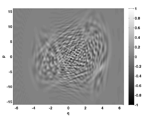
Figure 1: Phase space rendering of the Wigner function for the Duffing system at time $t=314~{}\mbox{periods of driving}$. The nonlocal interference is significant and cannot be associated with specific classical structures. This plot is taken at a relatively small $D$ value ($10^{-4}$) for resolution purposes. The value of $\hbar$ is set equal to 1 in order to clearly demonstrate this effect.

The most direct numerical test is a close examination of the time evolution of both the classical and quantum distribution functions for the quantum and dual classical evolutions. In this manner one can examine whether, over the expected timescales as predicted in the previous section, the expected phase space features are present for the template classical distributions and quantum Wigner functions.

A direct examination is necessary as other, seemingly logical measures, can sometimes be misleading. For instance, looking at expectation values is not always helpful. Typically, one would sample a set of lower order moments, and follow their expectation values for a desired amount of time. However, any classically chaotic system will have, over time, an infinite set of non-vanishing moments, as will any non-Gaussian quantum system gaussian . That said, one might attempt to argue that the effect of these higher-order moments may well be negligible. Even if this were the case, however, numerical simulations of chaotic systems have failed to find well-defined break times at which even lower-order moments permanently separate, and expectation values can agree well for surprisingly long timescales and even without the presence of environmental noise heller . Other measures, such as suppression of the integrated negativity of the Wigner function, also are not necessarily signatures of quantum-classical correspondence, as shown in Ref. hjmrss . Once the amount of negativity is eliminated via environmental decoherence, it was shown by these authors that the quantum evolution of a system may still disagree with its classical counterpart.

VI.1 Numerical Methods

Numerical solutions of the quantum master equation (19) for the Wigner function and of the corresponding dual classical Fokker-Planck equation were carried out using a split operator spectral method implemented on parallel supercomputers FF . The spectral method is particularly well-suited to high spatial resolution simulations where spatial structure is cut off above some given wavenumber – this is the case here for both the quantum and dual classical evolutions.

The time-stepping strategy is the same as that in analogous classical symplectic integrators. Suppose the time evolution of a function, $f(t)$, satisfies the operator equation:

$$\frac{\partial f}{\partial t}=(\hat{L}_{A}+\hat{L}_{B})f,$$ (37)

where the separate evolutions given by $\hat{L}_{A}$ and $\hat{L}_{B}$ can be implemented exactly. The exact solution to this equation is given by:

$$f(t)=e^{(\hat{L}_{A}+\hat{L}_{B})t}f(0).$$ (38)

Since $\hat{L}_{A}$ and $\hat{L}_{B}$ do not commute in general, the fact that the individual evolutions are known exactly is not of direct use. An integration scheme for a small timestep $\Delta t$ can be constructed simply, however, using the Campbell-Baker-Hausdorff theorem:

$$f(\Delta t)\approx e^{(\frac{\Delta t}{2}\hat{L}_{A})}e^{(\Delta t\hat{L}_{B})}e^{(\frac{\Delta t}{2}\hat{L}_{A})}f(0)+O(\Delta t^{3}).$$ (39)

With the assumption that the exponentiated operators can be applied exactly, this method is accurate to second order in $\Delta t$. The third order correction term is

$$\frac{1}{24}(\Delta t)^{3}[\hat{L}_{A}+2\hat{L}_{B},[\hat{L}_{A},\hat{L}_{B}]]f(0),$$ (40)

which can be evaluated to estimate the accuracy of the approximation.

In the present case, the evolution operator is $\hat{L}_{cl}+\hat{L}_{q}+D\partial^{2}_{p}$ for the Wigner evolution and is the same, but with $\hat{L}_{q}=0$ for the dual classical evolution. We split this into three operators, the “stream” operator $-(p/m)\partial_{q}$, the “kick” operator proportional to potential derivatives, which differs for the classical and quantum cases, and the momentum diffusion operator. As each piece involves either derivatives of position or momentum, but not both, the individual operators can be easily evaluated using a fast Fourier transform. The split-operator method preserves the unitarity of evolutions when $D=0$ and given a sufficient number of grid points in the spatial and momentum directions – satisfying associated Nyquist conditions – the operators can be evaluated at each timestep with essentially no spatial discretization error.

The typical mesh used over phase space consisted of 4096 by 4096 grid points. This size was determined by our need to resolve the bounded classical phase space portrait for the amount of time necessary to show long range agreement between the classical and quantum evolutions. If $D=0$, the classical phase space will be chaotic, and the system can only be explored for short times, before which structures begin to proliferate on scales smaller than the area defined by the grid spacing. The addition of an environmental interaction, as demonstrated in the theoretical section, prevents structures from forming on infinitely small scales. This makes it possible for the classical evolution to converge as resolution improves. The aforementioned grid-size is the one for which convergence was achieved for the systems we studied, and was derived empirically. Convergence for the quantum evolution is determined by the smallest scales – $\delta x=\hbar/P$ in space and $\delta p=\hbar/L$ in momentum – present in the Wigner function ($L$ and $P$ are the scales of the system boundaries in length and momentum, respectively). Thus, a typical mesh spacing can be fixed without regard to the strength of the environmental interaction. For our investigations, this required less resolution than in the classical phase space and, therefore, the dual classical evolution dictated the grid-size for the numerical simulations.

VI.2 Duffing Oscillator

The particular potential chosen for study was the chaotic Duffing oscillator with unit mass: $H(q,p,t)=p^{2}/2+Bx^{4}-Ax^{2}+\Lambda x\cos(\omega t)$. The evolution was evaluated for the set of parameters $A=\Lambda=10$, $B=0.5$ and $\omega=6.07$. In this parameter regime, the system is strongly chaotic, with an average Lyapunov exponent of $\bar{\lambda}=0.57$ that is relatively uniform over the hyperbolic phase space region Ball . The size of the bounded phase space region, which is $A$ in our calculations, is approximately $270$ units of action. The hyperbolic region of the system’s bounded motion is generated by the homoclinic tangle of a single hyperbolic fixed point and the stable regions are relatively small. Consequently, the unstable manifold associated with the hyperbolic point completely characterizes the chaotic region and provides an ideal test for the theory developed in this paper for bounded hyperbolic regions.

These parameters were chosen, not only because they provide appropriate testing conditions for theory, but also because their classical dynamics have been well studied in Ref. Ball and elsewhere. As a result, one can estimate the values of the quantities of interest, e.g., $t_{qc}$, with the system parameters, such as $\bar{\lambda}$, fixed at some canonical values. In addition, one also must be careful to choose a value of $\hbar$ which is not so large that the initial conditions are well outside the bounded region. Of course, choosing a value of $\hbar$ of the same order of magnitude as the bounded region or greater, would also invalidate the argument. One also does not want to choose $D$ values which are very large compared to those at which the transition is predicted to occur, as extreme $D$ values, while inducing quantum-classical correspondence, may wash out any intrinsic system dynamics.

We will principally focus on the case where $\hbar=0.1$ for a variety of practical reasons. The value of $\hbar=0.1$ turns out to be convenient for these purposes: the critical $D$ value predicted is small, but not too small that it is below computational resolution, and it also allows a wide range of $D$ values to be studied without smearing out the system dynamics. This value of $\hbar$ was used in Ref. SalKo which motivated much of this research, and which confirms that a weak transition will occur for this value. Still, the additional set of $\hbar$ values, $\{0.01,0.5,1,\sqrt{2},3,5,10,20\}$, were studied, and all revealed similar results, though some, such as $\hbar=0.01$ and $\hbar=5$, had compromised dynamical ranges, while $\hbar=10$ and $20$, were too large to be of practical interest. The results presented in depth in this section for $\hbar=0.1$ should, therefore, be thought of as emblematic of all cases studied. For a given trial, $\hbar$ and $D$ were held fixed.

We use the same normalized initial conditions for both dual classical and quantum evolutions, as we are trying to see the degree to which the two evolutions follow each other. In the numerical simulations, the typical condition was a superposition of two Gaussians, since a classically unacceptable initial condition would better illustrate the suppression of interference effects. Other conditions were also tried and compared, with analogous results.

The choice of $D=0.001$, yields the estimates $t^{*}=15.02$ and $t_{qc}=57$. For this case, the development of large scale classical structures should terminate before quantum and classical agreement occurs. A larger value for the diffusion coefficient, $D=0.01$, gives $t^{*}=13.1$ and $t_{qc}=5.7$. Here the transition occurs just before the termination of classical structure. Because of the quantum nature of the initial condition, in the estimation of $t^{*}$, we have set $u_{0}^{2}=\hbar$.

We now set out to test these predictions via numerical simulations. We first compare the classical and quantum evolutions at late times in order to establish whether or not a quantum-classical transition in fact occurs as predicted. Comparison of expectation values was helpful to establish whether the transition had occurred, but final approval was given only after examining the distribution functions and Wigner functions directly. Such a comparison is presented in Figure 2. We compare cross-sectional slices of the classical distribution function and quantum Wigner function after $149$ drive periods of the Duffing oscillator. These slices are taken along the $p=0$ line. For $D=10^{-5}$ very little agreement occurs between the classical and quantum slices (as expected, since in this case $t_{qc}\sim 5700$). In fact, the quantum slice still has many negative regions. For $D=10^{-3}$, in agreement with our order of magnitude estimate for when a transition should occur, progress has clearly been made. The two functions are in average agreement with one another, and, although there is less agreement on details, there is agreement between the two on some of the larger phase space feature. At a larger value, $D=10^{-2}$, this agreement is much improved and overall, the distributions are much smoother.

Note that the weak QCT occurs in time when $l_{q}=l_{cl}\sim\sqrt{\hbar}$, this phase space scale being independent of the value of $D$. However, the form of the large-scale classical template is determined by the structures present at $t^{*}$, which is sensitive to the value of $D$. Additionally, larger values of $D$ will lead to stronger filtering in both the quantum and classical cases. At a fixed value of time and $\hbar$, this means that slices of the Wigner function at higher $D$ values will have broader features and more efficient filtering of small scales. This aspect is clearly demonstrated in the three panels of Figure 2.

Figure 2: Sectional cuts of Wigner functions (dashed lines) and classical distributions (solid lines) for a driven Duffing oscillator, after 149 drive periods, taken at $p=0$ for (a) $D=10^{-5}$; (b) $D=10^{-3}$; (c) $D=10^{-2}$. Parameter values are as stated in the text; the height is specified in scaled units.

We now examine the time-dependence in more detail. In Figure 3, we display cross-sectional slices taken at $t=10$ and $t=30$. At $t=10$, the slice in the top panel, the classical and quantum functions have still clearly not explored phase space sufficiently. The Wigner function, has significant negative values and the classical distribution function has not been heavily broken up by the dynamics. By $t=30$ (still less than $t_{qc}$), lower panel, the picture begins to resemble the late-time plot shown in Figure 2. The negative regions of the Wigner function have been largely eliminated and the functions are distributed throughout phase space and are in approximate agreement. This result is also consistent with the estimated value of $t_{qc}$.

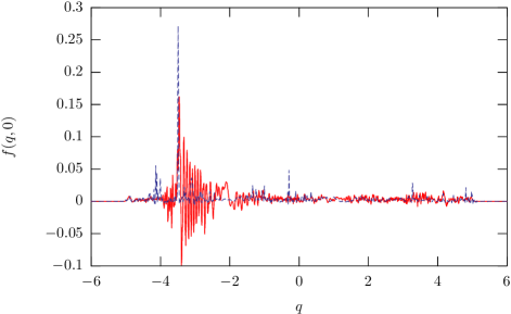
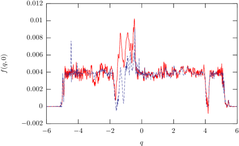
Figure 3: Cross-sectional slices of the Wigner function (red) and classical distribution function (blue) taken in phase space for $p=0$ and $D=10^{-3}$. The higher plot is taken at $t=10$ and the lower plot is taken at $t=30$.

We now perform a similar analysis for $D=10^{-2}$, for which $t_{qc}$ is an order of magnitude shorter. The top panel of Figure 4 is a snapshot at $t=8$, close to $t_{qc}$, whereas the lower plot is taken at the later time $t=20$. The early-time panel shows that the two distributions closely agree on general features of the dynamics, as predicted. By $t=20$, the weak QCT is well-stabilized, and one sees the strong agreement on most individual features present in the late-time case shown in Figure 2.

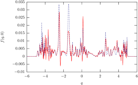
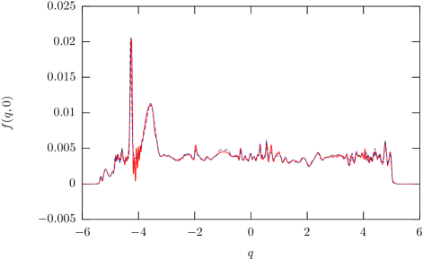
Figure 4: Cross-sectional slices of the Wigner function (red) and classical distribution function (blue) taken in phase space for $p=0$ and $D=10^{-2}$. The higher plot is taken at $t=8$ and the lower plot is taken at $t=20$.

As indicated earlier, similar results were seen at other values of $\hbar$, at the same level of detail shown here for $\hbar=0.1$. Many of the studies of the late-time dynamics of this system appear in Ref. BenPhD . As a further example, we show plots in Figure 5 for the case of $\hbar=1$ and with stronger noise coupling than the typical case considered in the theoretical analysis. In the upper panel $D=0.1$, while the lower plot has $D=1$; the snapshots are taken at $t=20$. (In both cases, $t_{qc}<t^{*}$.) The top slice shows general agreement between the two distributions, with some residual quantum interference effects. When $D=1$, the formal value of $t_{qc}$ is less than the dynamical timescale. This indicates that the onset of the weak QCT should be very rapid and by the relatively late time at which the snapshot is taken, the transition should be complete. The numerical results are very consistent with this prediction. These two plots show that even in the regime where our formal analysis might break down (large $\hbar$, large $D$), the general features and timescales follow the predicted estimates. At even larger (unphysical) values of $\hbar$ and $D$, the phase space boundaries become important and the smoothing gets so large that dynamical features hardly survive in the distributions.

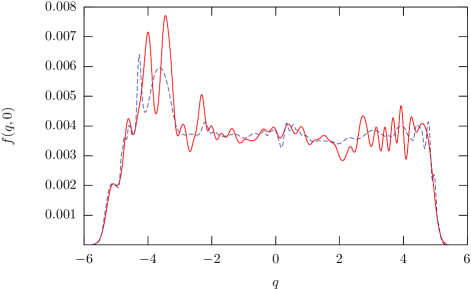
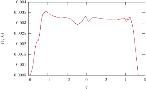
Figure 5: Cross-sectional slices of the Wigner function (red) and classical distribution function (blue) following Figure 4. The upper panel has $D=0.1$ and the lower panel, $D=1$. Both snapshots are taken for at $t=20$.

Finally, we address one last point of the argument – that the noise-averaged termination of fine scale structure would lead to the presence of the early time folding associated with the foliation of the unstable manifold generated by the homoclinic point of the Duffing system. Evidence for this is presented in Figure 7, a full late-time, high-resolution phase space rendering of the Wigner function for $D=10^{-3}$. The time is taken to be $t=149$ (roughly a factor of two greater than $t_{qc}$), well after the quantum-classical transition has occurred. Superimposed on the Wigner function is the early time unstable manifold. It is clear that the evolution has organized along these early-time features, as expected from our analysis. The final distribution which both the dual classical distribution and Wigner function approach, once the transition has occurred, shows the suppression of the late-time, fine-scale features of the unstable manifold, as it is supported by the large early-time structures. Quantum interference, while expected, is local and is strongest near the sharp turns in the manifold where branches are most close together. This, combined with the previous results in this section, allow us to conclude that the basic mechanisms posited for the quantum-classical transition are consistent with results from numerical simulations.

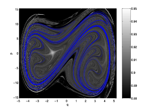
Figure 6: Phase space rendering of the Wigner function at time $t=149$ periods of driving. The early-time part of the unstable manifold associated with the noise-free dynamics is shown in blue (see text for discussion). The value of $D=10^{-3}$ is not sufficient to wipe out all the quantum interference which, as expected, is most prominent near sharp turns in the manifold.

VII Conclusion and Future Directions

We have presented a set of physical mechanisms which explain the source of the weak quantum-classical transition for one-dimensional, bounded chaotic systems. The fact that one-dimensional, chaotic systems are being investigated in real world laboratory experiments, with interesting potential applications, further enhances the importance of understanding how unconditioned environmental interactions affect a subsystem of interest. We have used this understanding to derive estimates for the time at which the weak transition occurs.

It is important to keep in mind that currently there is no general understanding of which systems will actually exhibit a weak QCT, so the existence of this timescale has another useful feature, in terms of classification of quantum dynamical systems. If a weak QCT has not occurred by the predicted $t_{qc}$, our analysis would argue that it will not occur at all (within the parametric assumptions made). So the existence or nonexistence of this time can be used as a test for the occurrence of long-time quantum-classical correspondence (but still on timescales shorter than the physical equilibration timescale) without any knowledge of initial conditions.

Our numerical results illustrated the compact manifold structure induced by the bounded phase space region. The role of boundedness is a key component in the theoretical analysis presented earlier in this paper. This topological feature causes the system to fold on itself, which, in turn, allowed us to estimate a timescale for the termination of fine structure. A one-dimensional bounded chaotic evolution, coupled with noise, appears to necessarily terminate fine scale structure. In order for the analysis to be valid, the system must be bounded or, if it is unbounded, it must at least fold onto itself in such a way as to allow a similar process to take place. The lack of such an evolution may be a reason why no such transition was found for the manifestly unbounded delta-kicked rotor studied in Ref. bhjs . Additionally, while an unconditioned evolution eliminated all negativity from the quantum Wigner function, the distribution was still not classical hjmrss .

It is useful to restate the ways in which the present analysis differs from previous work. First, the connection to continuous measurement and the weak and strong forms of quantum-classical correspondence are explicitly stated. Second, we use the dual classical Fokker-Planck equation not to represent a physical classical evolution, but rather as a dynamical foil of the open-system quantum evolution, one that can handle quantum initial states, and quantum backaction (which is missing in classical theory), but keeps only the classical system propagator. Third, our analysis is symmetric – we consider the effect of noise acting as a filter on the open-system quantum evolution (treated in semiclassical approximation) melded with a consideration of noise-induced filtering on the classical dual evolution with its exponential-in-time folding of phase space structures characteristic of chaos. This folding points to the role of global phase-space topology in deriving our results, and distinguishes them from local, heuristic analyses of the role of decoherence in the quantum to classical transition ZP .

Clearly, more work is needed to fully explore the conditions under which the weak QCT exists, especially the role of boundedness. In this regard, investigation of two-dimensional systems would be informative as several of the topological arguments presented here would likely need to be modified. Adding more dimensions would introduce effects such as Arnold diffusion which become important components of the dynamics. Many of these features lack a lower dimensional analog, so it is reasonable to believe that they could play an important role in the higher dimensional QCT. It would also be interesting to see what qualitative features of the weak quantum to classical transition will be preserved in these systems. More immediately, the connection between the requirements for weak and strong QCT scenarios are worth contrasting, especially to delineate parameters regimes for validity. This project is currently underway bkbk .

Numerical simulations were performed on the Cray T3E and IBM SP3 at NERSC, LBNL. B.D.G. and S.H. acknowledge support from the LDRD program at LANL. B.D.G. was also partially supported by the Center for Nonlinear Studies at LANL. The work of B.S. and B.D.G (partially) was supported by the National Science Foundation grant #0099431.

References

- (1) L. Landau and E.M. Lifshitz, Quantum Mechanics: Non-Relativistic Theory (Pergamon Press, New York, 1965).
- (2) A. Einstein, Verh. Dtsch. Phys. Ges. 19, 82 (1917); M. Born, The Mechanics of the Atom (G. Bell, London, 1927).
- (3) A.J. Dragt and S. Habib, Proceedings of the Advanced Beam Dynamics Workshop on Quantum Aspects of Beam Physics, (Monterey, 1998), edited by P. Chen (World-Scientific, 1999).
- (4) S. Habib, K. Jacobs, H. Mabuchi, R. Ryne, K. Shizume, and B. Sundaram, Phys. Rev. Lett. 88, 040402 (2002).
- (5) M.V. Berry and N.L. Balazs, J. Phys. A. 12, 625 (1979); G.P. Berman and G.M. Zaslavsky, Physica A 91, 450 (1978); G.M. Zaslavsky. Phys. Rep. 80, 157 (1981).
- (6) S. Tomsovic and E.J. Heller, Phys. Rev. Lett. 67, 664, (1991); Phys. Rev. E 47, 282 (1993).
- (7) J. Ford, G. Mantica, and G.H. Ristow, Physica D 50, 493 (1991); J. Ford and G. Mantica, Am. J. Phys. 60, 1086 (1992).
- (8) D.N. Spergel, et. al, Astrophys. J. Supp. Ser. 148, 1 (2003); 148, 175 (2003).
- (9) B.V. Chirikov, Chaos 1, 95 (1991); S. Habib, et. al, Ann. N.Y. Acad. Sci. 1045, 308 (2005).
- (10) H.J. Carmichael, An Open Systems Approach to Quantum Optics (Springer, 1993); C.W. Gardiner and P. Zoller, Quantum Noise (Springer, 2000); M. Orszag, Quantum Optics (Springer, 2000).
- (11) H.M. Wiseman, Ph.D. thesis, University of Queensland, 1994.
- (12) S. Habib, et. al., Proc. NATO Advanced Workshop, Nonlinear Dynamics and Fundamental Interactions, (Tashkent, October 2004), edited by F. Khanna and D. Matrasulov (Springer, 2006).
- (13) C.M. Caves and G.J. Milburn. Phys. Rev. A 36, 5543 (1987).
- (14) G. Lindblad, Comm. Math. Phys. 48, 119 (1976); V. Gorini and A. Kossakowski, J. Math. Phys. 17, 1298 (1976).
- (15) S. Habib, K. Shizume, and W.H. Zurek. Phys. Rev. Lett. 80, 4361 (1998).
- (16) T. Bhattacharya, S. Habib, and K. Jacobs, Phys. Rev. Lett. 85, 4852 (2000).
- (17) S. Habib, K. Jacobs, and K. Shizume. Phys. Rev. Lett. 96, 010403 (2006).
- (18) T. Bhattacharya, S. Habib, K. Jacobs, and K. Shizume, Phys. Rev. A 65, 032115 (2002).
- (19) B.D. Greenbaum, S. Habib, K. Shizume, and B. Sundaram, Chaos 15, 033302 (2005).
- (20) A.R.R. Carvalho, et al., Phys. Rev. E 70, 026211 (2004).
- (21) G. Voth, G. Haller, and J.P. Gollub, Phys. Rev. Lett. 88, 254501 (2002).
- (22) M.V. Berry, Phil. Trans. Roy. Soc. London. A 287, 237 (1977).
- (23) B.D. Greenbaum, Ph.D. Thesis, Columbia University, 2006.
- (24) E.P. Wigner, Phys. Rev. 40, 749 (1932).
- (25) M. Hillery, R. O’Connell, M.O. Scully, and E.P. Wigner. Phys. Rep. 106, 121 (1984); V.I. Tatarskii, Sov. Phys. Usp. 26, 311 (1983).
- (26) L.E. Ballentine, Quantum Mechanics: A Modern Development (World Scientific, Singapore, 1998).
- (27) K. Husimi, Proc. Phys. Math. Soc. Jpn. 55, 762 (1940).
- (28) K. Takahashi and N. Saito, Phys. Rev. Lett. 55, 645 (1985); D. Lalovic̀, D. M. Davidović, and N. Bijedić, Phys. Rev. A 46, 1206 (1992).
- (29) For example, L.I. Schiff, Quantum Mechanics (McGraw-Hill, New York, 1968), 3rd ed.; B.H. Brandsen and C.J. Joachain, Introduction To Quantum Mechanics (Prentice Hall, New York, 2000).
- (30) V.P. Maslov and M.V. Fedoriuk, Semi-Classical Approximation in Quantum Mechanics (Dordrecht, Holland, 1981).
- (31) C. Bender and S. Orszag, Advanced Mathematical Methods for Scientists and Engineers (McGraw Hill, New York, 1978).
- (32) G. Chester, B. Friedman, and F. Ursell, Proc. Camb. Phil. Soc. 53, 599 (1957).
- (33) For a clear derivation and discussion, including many relevant references, see K. Jacobs and D.A. Steck, Cont. Phys. 47, 279 (2006). See also G.J. Milburn, Quant. Semiclass. Opt. 8, 269 (1996).
- (34) A.O. Caldeira and A.J. Leggett, Phys. Rev. E 121, 587 (1983); A.O. Caldeira, H.A. Cerdeira, and R. Ramaswamy, Phys. Rev. A 40, 3438 (1989).
- (35) C.W. Gardiner, Handbook of Stochastic Methods (Springer-Verlag, Berlin, 1997).
- (36) N.G. Van Kampen, Stochastic Processes in Physics and Chemistry (Elsevier North Holland, New York, 1983).
- (37) W. Liu and G. Haller, Physica D. 188, 1 (2004).
- (38) A.R. Kolovsky, Phys. Rev. Lett. 76, 340 (1996).
- (39) S. Habib, quant-ph/0406011 (2004).
- (40) M.D. Feit, J.A. Fleck, Jr., and A. Steiger, J. Comp. Phys. 47, 412 (1982).
- (41) W.A. Lin and L.E. Ballentine, Phys. Rev. Lett. 65, 2927 (1990).
- (42) W.H. Zurek and J.P. Paz. Phys. Rev. Lett. 72, 2508 (1994). Physica D, 83, 300 (1995).
- (43) B.D. Greenbaum, K. Jacobs, and B. Sundaram, in preparation.