Long-range entanglement in the Dirac vacuum

Abstract

Recently, there have been a number of works investigating the entanglement properties of distinct noncomplementary parts of discrete and continuous Bosonic systems in ground and thermal states. The Fermionic case, however, has yet to be expressly addressed. In this paper we investigate the entanglement between a pair of far-apart regions of the 3+1 dimensional massless Dirac vacuum via a previously introduced distillation protocol [B. Reznik, et al., Phys. Rev. A 71, 042104 (2005)]. We show that entanglement persists over arbitrary distances, and that as a function of $L/R$, where $L$ is the distance between the regions and $R$ is their typical scale, it decays no faster than $\sim exp\left[-\left(L/R\right)^{2}\right]$. We discuss the similarities and differences with analogous results obtained for the massless Klein-Gordon vacuum.

School of Physics and Astronomy, Raymond and Beverly Sackler Faculty of Exact Sciences, Department of Physics and Astronomy, Tel-Aviv University, Tel-Aviv 69978, Israel

Entanglement in spatially extended many body systems and quantum field theories is the focus of increasing attention. Part of this is directed at understanding the entanglement properties of noncomplementary parts of a system, such as far apart regions of vacuum [1, 2, 3, 4, 5] and thermal states [6, 7], or widely separated segments in ground states of the Bose-Hubbard Hamiltonian [8], chains of trapped ions [9] and harmonic oscillators [10]. In this regard relativistic vacua are especially interesting as they provide us with an oppurtunity to study physical systems with a well defined notion of locality.

In this paper we investigate the entanglement between arbitrarily distant regions of the free massless Dirac vacuum. For Bosonic systems, the expansion of the vacuum in terms of two-mode squeezed states of oscillators residing in the two complementary spacetime wedges $x>0$ and $x<0$, used in the derivation of the Unruh effect, explicitly shows that the vacuum is entangled [11, 12]. This result is a special case of a general modewise decomposition theorem pertaining to a certain class of Bosonic Gaussian states [13, 14]. An analogous theorem exists for Fermionic Gaussian states [15]. (Indeed, the Unruh effect holds also in the Fermionic vacuum [16].) The state of a pair of noncomplementary parts of a system, however, in general is mixed, so that a modewise decomposition is impossible [17]. Working directly with the system’s degrees of freedom, especially when of a great or inifinite number, proves difficult then. A most effective and relatively simple way to tackle this problem is the use of entanglement distillation protocols. Even though such protocols have proved most convenient in the study of the entanglement between abitrarily distant regions of the Bosonic vacuum [3, 4, 5], the Fermionic case has thus far not been expressly addressed. Using a previously introduced distillation protocol [2, 3], we explicitly show that results analogous to those obtained for the Bosonic vacuum are true of the Fermionic vacuum as well, namely, that entanglement persists between arbitrarily far-apart regions and that as a function of the ratio of the separation between the regions $L$ and their typical scale $R$, the entanglement decays no faster than $\sim exp\left[-\left(L/R\right)^{2}\right]$.

The concepts of entanglement and locality are nontrivial in Fermionic systems. We therefore begin by explaining them briefly and contrast with the Bosonic case. Suppose we have a system of Bosonic modes. As $\left[a_{i},\,a_{j}^{\dagger}\right]=\delta_{ij}$ and $\left[a_{i},\,a_{j}\right]=0$, the Hilbert space is a direct product of the Hilbert spaces of each of the modes. Hence, it is meaningful to consider the entanglement between different sets of modes, with the partition unequivocally defining locality. For Fermions $\left\{a_{i},\,a_{j}^{\dagger}\right\}=\delta_{ij}$ and $\left\{a_{i},\,a_{j}\right\}=0$. The Hilbert space therefore lacks an analogous direct product structure. If the assignation of sets of modes to different parties is to have any meaning at all (that is, if we do not want to give up locality), we must restrict the set of observables in such a way that acting on an arbitrary composite state of any two distinct sets of modes, say $A$ and $B$, with an observable comprised solely of modes in $A$, does not change the expectation values of any observable comprised solely of modes in $B$ (and vice-versa), nor increase the entanglement between the sets. Now, let $\hat{O}_{A}$ and $\hat{O}_{B}$ be arbitrary sums of products of even number of modes in $A$ and $B$, respectively, then $\left[\hat{O}_{A},\,\hat{O}_{B}\right]=0$. It is not hard to see that this characteristic of Fermionic modes, together with the anti-commutation algebra of the modes, restricts the set of observables to those that can be constructed out of products of an even number of modes [18]. For pure states entanglement between two sets of modes is then defined as usual, i.e. a pure composite state of two sets of modes, $\phi$, is entangled iff there exist observables $\hat{O}_{A}$ and $\hat{O}_{B}$ such that $\left\langle\hat{O}_{A}\hat{O}_{B}\right\rangle_{\phi}\neq\left\langle\hat{O}_{A}\right\rangle_{\phi}\left\langle\hat{O}_{B}\right\rangle_{\phi}$. Of course this is not true of mixed states. Indeed, except in $2\times 2$ and $2\times 3$ dimensions [19, 20], no necessary and sufficient criterion to establish mixed state entanglement is known, regardless of the statistics.

Moving on to relativistic quantum field theory (QFT), the requirement of Lorentz covariance and that the energy spectrum be bounded from below constrains the set of possible algebras of modes to the familiar commutation/anti-commutation relations for Bosons/Fermions. As an example consider the Dirac field

$$\left\{\psi_{i}\left(\vec{x},\,t\right),\,\psi_{j}^{\dagger}\left(\vec{y},\,t\right)\right\}=\delta_{ij}\delta\left(\vec{x}-\vec{y}\right),\qquad\left\{\psi_{i}\left(\vec{x},\,t\right),\,\psi_{j}\left(\vec{y},\,t\right)\right\}=0.$$ (1)

The subscripts denote the spinorial indices, which together with the position $\vec{x}$ label the modes. If in addition we want the theory to be causal, we must require that observables be respresented by bilinear expressions in the fields.

It is important to note that there is a difference in what is meant by “local” in quantum information theory (QIT) and QFT settings. As explained above, in QIT it is the different parties that define locality. However, in QFT it is causality which defines locality, i.e. an operator acting at two or more spacelike related coordinates is nonlocal. In this paper, locality in the QIT sense enters via the assignation of causally disconnected regions to different parties, leaving us with much greater latitude in our choice of “local” operations than that afforded by the tight constraints of QFT.

The protocol employed in [2, 3] consists of the finite duration coupling of a pair of initially nonentangled two-level point-like detectors to the studied field, in its vacuum state, at two different locations. The duration of the coupling determines the size of the regions “probed” and is taken to be much smaller than the distance between the detectors, which therefore remain causally disconnected. Under these conditions, a final entangled state of the detectors means that entanglement persists between the regions. A similar but suitably adjusted protocol is employed here. We therefore make use many of the results obtained in [3], and forego rederivation.

The Dirac equation is given by

$$\left(\vec{\alpha}\cdot\vec{p}+\beta m\right)\psi\left(\vec{x},\,t\right)=i\frac{\partial}{\partial t}\psi\left(\vec{x},\,t\right),$$ (2)

where the $\alpha_{i}$ and $\beta$ are any $4\times 4$ matrices satisfying $\left\{\alpha_{i},\,\alpha_{j}\right\}=2\delta_{ij}\mathbf{1}$, $\beta^{2}=\mathbf{1}$, and $\left\{\alpha,\,\beta\right\}=0$. In the absence of a mass term, in the Weyl representation of the $\alpha_{i}$ and $\beta$, the Dirac equation decouples into a pair of equations, the Weyl equations

$$\vec{\sigma}\cdot\vec{p}\,\psi_{r}\left(\vec{x},\,t\right)=i\frac{\partial}{\partial t}\psi_{r}\left(\vec{x},\,t\right),\qquad-\vec{\sigma}\cdot\vec{p}\,\psi_{l}\left(\vec{x},\,t\right)=i\frac{\partial}{\partial t}\psi_{l}\left(\vec{x},\,t\right),$$ (3)

where the $\sigma_{i}$ are the Pauli matrices. The two-component fields $\psi_{r}\left(\vec{x},\,t\right)$ and $\psi_{l}\left(\vec{x},\,t\right)$ describe right and left handed particles and anti-particles, that is quanta of positive and negative helicity, respectively. We can therefore begin by studying a vacuum of definite handedness, say the right handed vacuum. In terms of a Fourier expansion

$$\psi_{r}\left(\vec{x},\,t\right)=\int\frac{d^{3}p}{\left(2\pi\right)^{3}}\left(a_{\vec{p}}^{r}u_{r}\left(\vec{p}\right)e^{-i\left(pt-\vec{p}\cdot\vec{x}\right)}+\left.b_{\vec{p}}^{r}\right.^{\dagger}v_{r}\left(\vec{p}\right)e^{i\left(pt-\vec{p}\cdot\vec{x}\right)}\right).$$ (4)

$\left.a_{\vec{p}}^{r}\right.^{\dagger}$, $a_{\vec{p}}^{r}$ and $\left.b_{\vec{p}}^{r}\right.^{\dagger}$, $b_{\vec{p}}^{r}$ are the creation and annihilation operators for right handed particles and anti-particles, respectively, satisfying $\left\{a_{\vec{p}}^{r},\,\left.a_{\vec{p}}^{r}\right.^{\dagger}\right\}=\left\{b_{\vec{p}}^{r},\,\left.b_{\vec{p}}^{r}\right.^{\dagger}\right\}=\left(2\pi\right)^{3}\delta\left(\vec{p}-\vec{q}\right)$ with all other anti-commutators vanishing, while $u_{r}\left(\vec{p}\right)$ and $v_{r}\left(\vec{p}\right)$ are the corresponding two-component “spinorial” coefficients and are understood to be normalised to unity.

Due to the fact that the field is Fermionic, we must couple to field bilinears to realise the distillation protocol [3]. (See earlier discussion.) Perhaps the most natural choice is the field’s charge density $\hat{N}\left(\psi_{r}^{\dagger}\left(\vec{x}_{i},\,t\right)\psi_{r}\left(\vec{x}_{i},\,t\right)\right)$, where for convenience we have chosen to normal order ($\hat{N}$). Setting up a pair of two-level detectors at $\vec{x}_{A}$and $\vec{x}_{B}$, in the Dirac interaction picture the coupling term is given by

$$H_{C}\left(t\right)=\frac{1}{2}\sum_{i=A,\,B}\epsilon_{i}\left(t\right)\left(Cos\left(\Omega_{i}t\right)\sigma_{i}^{x}+Sin\left(\Omega_{i}t\right)\sigma_{i}^{y}\right)\hat{N}\left(\psi_{r}^{\dagger}\left(\vec{x}_{i},\,t\right)\psi_{r}\left(\vec{x}_{i},\,t\right)\right).$$ (5)

Here $\epsilon_{i}\left(t\right)$ governs the strength and duration of the coupling, and $\Omega_{i}$ is the energy gap of detector $i$. The corresponding evolution operator is $U\left(T/2\right)=\hat{T}exp\left[-i\int_{-T/2}^{T/2}dtH_{C}\left(t\right)\right]$, with $\hat{T}$ and $T$ denoting time-ordering and the duration of the interaction, respectively. As discussed above, we set $L\gg T$ ($L:=\left|\vec{x}_{B}-\vec{x}_{A}\right|$), and take the initial state of the detectors to be separable.

Once the interaction is over, in the basis $\left\{\downarrow\downarrow,\,\downarrow\uparrow,\,\uparrow\downarrow,\,\uparrow\uparrow\right\}$, the partial transpose of the detectors’ reduced density matrix is given by

$$\rho_{AB}^{PT}=\left(\begin{array}[]{cccc}1-\left\|E_{A}\right\|^{2}-\left\|E_{B}\right\|^{2}&0&0&\left\langle E_{A}\mid E_{B}\right\rangle\\ 0&\left\|E_{B}\right\|^{2}&-\left\langle 0\mid X_{AB}\right\rangle&0\\ 0&-\left\langle X_{AB}\mid 0\right\rangle&\left\|E_{A}\right\|^{2}&0\\ \left\langle E_{B}\mid E_{A}\right\rangle&0&0&\left\|X_{AB}\right\|^{2}\end{array}\right)+O\left(\epsilon_{i}^{3}\right),$$ (6)

where

$$\left|E_{i}\right\rangle:=\int_{-T/2}^{T/2}dt\epsilon_{i}\left(t\right)e^{i\Omega_{i}t}\hat{N}\left(\psi_{r}^{\dagger}\left(\vec{x}_{i},\,t\right)\psi_{r}\left(\vec{x}_{i},\,t\right)\right)\left|0\right\rangle,$$ (7)

$$\left|X_{AB}\right\rangle:=\int_{-T/2}^{T/2}dtdt^{\prime}\epsilon_{A}\left(t\right)\epsilon_{B}\left(t^{\prime}\right)e^{i\left(\Omega_{A}t+\Omega_{B}t^{\prime}\right)}\hat{N}\left(\psi_{r}^{\dagger}\left(\vec{x}_{A},\,t\right)\psi_{r}\left(\vec{x}_{A},\,t\right)\right)\hat{N}\left(\psi_{r}^{\dagger}\left(\vec{x}_{B},\,t^{\prime}\right)\psi_{r}\left(\vec{x}_{B},\,t^{\prime}\right)\right)\left|0\right\rangle.$$ (8)

Using the Peres criterion [19], we find that the detectors are entangled (i.e. that the partial transpose has negative eigenvalues) if

$$\left|\left\langle 0\mid X_{AB}\right\rangle\right|^{2}-\left\|E_{A}\right\|^{2}\left\|E_{B}\right\|^{2}>0.$$ (9)

Physically speaking, this translates to the requirement that the probability of exchange of a right handed virtual particle - anti-particle pair between the detectors be greater than the product of the probabilities for the on-shell emission of a right handed particle - anti-particle pair by the same detector.

For temporally symmetric window functions, a somewhat lengthy calculation shows that the above condition takes on the explicit form (see appendix for details)

$$\left|\int_{0}^{\infty}\frac{d\omega}{L^{2}}\omega^{3}Cos\left(\omega L\right)\tilde{\epsilon}_{A}\left(\Omega_{A}+\omega\right)\tilde{\epsilon}_{B}\left(\Omega_{B}-\omega\right)+6\int_{0}^{\infty}\frac{d\omega_{1}d\omega_{2}}{L^{3}}\left[\frac{1}{L}Sin\left(\omega_{1}L\right)Sin\left(\omega_{2}L\right)\right.\right.$$

$$-\omega_{1}Cos\left(\omega_{1}L\right)Sin\left(\omega_{2}L\right)-\omega_{2}Sin\left(\omega_{1}L\right)Cos\left(\omega_{2}L\right)\bigg{]}\tilde{\epsilon}_{A}\left(\Omega_{A}+\omega_{1}+\omega_{2}\right)\tilde{\epsilon}_{B}\left(\Omega_{B}-\omega_{1}-\omega_{2}\right)\bigg{|}^{2} >$$

$$\frac{1}{25}\int_{0}^{\infty}d\omega\omega^{5}\tilde{\epsilon}_{A}\left(\Omega_{A}+\omega\right)^{2}\int_{0}^{\infty}d\omega\omega^{5}\tilde{\epsilon}_{B}\left(\Omega_{B}+\omega\right)^{2},$$ (10)

where $\tilde{\epsilon}_{i}$ is the Fourier transform of $\epsilon_{i}$.

This is to be compared with the condition obtained for the massless real Klein-Gordon field [2]

$$\left|\int_{0}^{\infty}\frac{d\omega}{L}Sin\left(\omega L\right)\tilde{\epsilon}_{A}\left(\Omega_{A}+\omega\right)\tilde{\epsilon}_{B}\left(\Omega_{B}-\omega\right)\right|^{2}>\int_{0}^{\infty}d\omega\omega\left|\tilde{\epsilon}_{A}\left(\Omega_{A}+\omega\right)\right|^{2}\int_{0}^{\infty}d\omega\omega\left|\tilde{\epsilon}_{B}\left(\Omega_{B}+\omega\right)\right|^{2}$$ (11)

The two conditions bear similarity. The analysis performed in [3] shows that Eq. (11) can be satisfied if we choose $\tilde{\epsilon}_{A}\left(\Omega_{A}-\omega\right)$ such that it oscillates as $Sin\left(\omega L\right)$, that is faster than any of its Fourier components, over a finite integration regime [23, 24]. Indeed, such a choice [25] can render the exchange probability arbitrarily larger than the product of the emission probabilities. Suppose in our case we take the superoscillatory transform to oscillate like $Cos\left(\omega L\right)$ over a suitably chosen integration regime. Then the specially tailored form of the superoscillatory transform guarantees that the first term on the LHS of Eq. (10) is much greater than the RHS. But for precisely the same reason it is much greater than all other terms on the LHS, and Eq. (10) is satisfied. It follows that entanglement persists between arbitrarily far-apart regions of the massless Dirac vacuum of quanta of definite handedness, and that the lower bound obtained in [3] holds here as well. That is, in the limit $L/T\gg 1$ the entanglement, quantified by the negativity $\mathcal{N}$, scales no faster than $\sim exp\left[-\left(L/T\right)^{2}\right]$. Now as in the duration $T$ the detectors probe a spherical region of radius $R=T$ (see Fig. 1), we arrive at the aforementioned lower bound $\sim exp\left[-\left(L/R\right)^{2}\right]$.

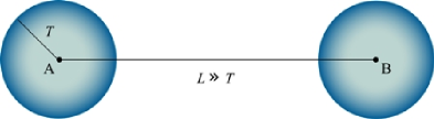
Figure 1: Spacetime at the start of the interaction $t=-T/2.$ $A$ and $B$ denote the locations of the detectors. It is only operators within the two spheres that contribute to the distilled entanglement.

Not surpirsingly, for the left handed vacuum the condition for entanglement is identical. This means that double the amount of entanglement can be distilled by coupling to the total charge density, that is the sum of the charge densities of right and left handed quanta.

Before we conclude, there are three questions that need to be addressed. First, as previously mentioned, an identical bound for the entanglement obtains for the Klein-Gordon vacuum. The question arises as to whether this reflects some sort of universality or is just an artifact of our distillation protocol [26]. Naively, it might be expected that the comparatively “poorer” structure of the Dirac Hilbert space, resulting from the anti-commutative nature of the field, leads to a faster decay. However, the fact that our distillation protocol is perturbative means that in the Klein-Gordon field case, the Hilbert space’s full structure does not come into play. This may very well be the reason for the identical bound, but to say more would be pure speculation.

Second, it is natural to ask whether the correlations giving rise to this entanglement can be attributed to a local hidden-variable model. In the Klein-Gordon field case, we were able to show [3] the detector’s final state exhibits “hidden” nonlocal correlations [27], in the sense that after local filtering [28] an EPR state can be distilled. However, the same does not true here, due to the presence of $\epsilon_{i}^{3}$ terms in the reduced density matrix, Eq. (6), not present in the Bosonic equivalent, which prevent the distillation of an EPR state. This question therefore remains open.

The third question is how the results obtained change in the massive case. Obviously, the presence of a mass term adds another scale to the problem. From the point of view of our distillation protocol, the Dirac equation no longer decouples and it is hard to see how use can be made of a superoscillating function to satisfy the resulting inequalities (without which we do not know how to distill entanglement at arbitrarily long distances). Nonetheless, the fact that the main contribution to the entanglement arises from high frequencies (see [3]) suggests that for a comparatively small mass our results should remain unchanged [29].

Appendix: Details of calculations

To clarify some of the physical content behind the condition for entanglement, Eq. (10), we outline here the important steps in its derivation.

As already noted, in the absence of a mass term, the Dirac equation decouples into a pair of equations for quanta of a definite handedness. However, it is only in the Weyl representation of the Gamma matrices

$$\gamma_{0}=\left(\begin{array}[]{cc}\mathbf{0}&\mathbf{1}\\ \mathbf{1}&\mathbf{0}\end{array}\right),\qquad\gamma_{i}=\left(\begin{array}[]{cc}\mathbf{0}&\sigma_{i}\\ \sigma_{i}&\mathbf{0}\end{array}\right),$$ (12)

that these equations reduce from four component equations to two. Taking the spinors to be normalised to unity we then have

$$u_{r}\left(\vec{p}\right)=v_{r}\left(\vec{p}\right)=\frac{1}{\sqrt{2p\left(p-p_{z}\right)}}\left(\begin{array}[]{c}p_{x}-ip_{y}\\ p-p_{z}\end{array}\right),\qquad u_{l}\left(\vec{p}\right)=v_{l}\left(\vec{p}\right)=u_{r}\left(-\vec{p}\right).$$ (13)

Focusing on the right handed vacuum, in terms of the Fourier expansion of the field the emission and exchange terms are given by

$$\left\|E_{i}\right\|^{2}=\int\frac{d^{3}pd^{3}q}{\left(2\pi\right)^{6}}v_{r}^{\dagger}\left(\vec{q}\right)u_{r}\left(\vec{p}\right)u_{r}^{\dagger}\left(\vec{p}\right)v_{r}\left(\vec{q}\right)\left|\tilde{\epsilon}_{i}\left(\Omega_{i}+p+q\right)\right|^{2},$$ (14)

$$\left\langle 0\mid X_{AB}\right\rangle=-\int\frac{d^{3}pd^{3}q}{\left(2\pi\right)^{6}}v_{r}^{\dagger}\left(\vec{p}\right)u_{r}\left(\vec{q}\right)u_{r}^{\dagger}\left(\vec{q}\right)v_{r}\left(\vec{p}\right)e^{i\left(\vec{p}+\vec{q}\right)\cdot\left(\vec{x}_{A}-\vec{x}_{B}\right)}\tilde{\epsilon}_{A}\left(\Omega_{A}+p+q\right)\tilde{\epsilon}_{B}\left(\Omega_{B}-p-q\right),$$ (15)

where we have already carried out the temporal integration. Plugging in the expressions for the spinors we get

$$\left\|E_{i}\right\|^{2}=\int\frac{d^{3}pd^{3}q}{\left(2\pi\right)^{6}}\frac{1}{2}\left(1+\frac{\vec{p}\cdot\vec{q}}{pq}\right)\left|\tilde{\epsilon}_{i}\left(\Omega_{i}+p+q\right)\right|^{2},$$ (16)

$$\left\langle 0\mid X_{AB}\right\rangle=-\int\frac{d^{3}pd^{3}q}{\left(2\pi\right)^{6}}\frac{1}{2}\left(1+\frac{\vec{p}\cdot\vec{q}}{pq}\right)e^{i\left(\vec{p}+\vec{q}\right)\cdot\left(\vec{x}_{A}-\vec{x}_{B}\right)}\tilde{\epsilon}_{A}\left(\Omega_{A}+p+q\right)\tilde{\epsilon}_{B}\left(\Omega_{B}-p-q\right).$$ (17)

In spherical coordinates the integration over angles is straightforward.

$$\left\|E_{i}\right\|^{2}=2\int_{0}^{\infty}\frac{dpdq}{\left(2\pi\right)^{4}}p^{2}q^{2}\left|\tilde{\epsilon}_{i}\left(\Omega_{i}+p+q\right)\right|^{2},$$ (18)

$$\left\langle 0\mid X_{AB}\right\rangle = -2\int_{0}^{\infty}\frac{dpdq}{\left(2\pi\right)^{4}}\frac{pq}{L^{2}}\left[Cos\left(\left(p+q\right)L\right)-\frac{p}{L}Cos\left(pL\right)Sin\left(qL\right)-\frac{q}{L}Sin\left(pL\right)Cos\left(qL\right)\right.$$ (19)

$$\left.+\frac{pq}{L^{2}}Sin\left(pL\right)Sin\left(qL\right)\right]\tilde{\epsilon}_{B}\left(\Omega_{A}+p+q\right)\tilde{\epsilon}_{B}\left(\Omega_{B}-p-q\right),$$

where $L:=\left|\vec{x}_{A}-\vec{x}_{B}\right|$. If we now switch to the variables $\omega=p+q$ and $\upsilon=p-q$, then integrating over $\upsilon$, Eq. (10) quickly follows.

We note that the $Cos\left(\omega L\right)$ term on the LHS of Eq. (10) arises from the angular integration over both the $\frac{1}{2}$ and $\frac{\vec{p}\cdot\vec{q}}{2pq}$ terms resulting from the spinor products. Were the $\frac{\vec{p}\cdot\vec{q}}{2pq}$ term absent, we would not be able to distill entanglement at any distance $L$. It is interesting that this implies that we cannot realise our distillation protocol in the real scalar vacuum via a square coupling.

Acknowledgments

We would like to thank J. Kupferman for useful discussions. This work was supported by the European Commission under the Integrated Project Qubit Applications (QAP) funded by the IST directorate as contract number 015848.

References

- [1] H. Halvorson and R. Clifton, J. Math. Phys. 41, 1711, (2000).
- [2] B. Reznik, quant-ph/0008006 (2000), and Found. Phys. 33, 167 (2003).
- [3] B. Reznik, A. Retzker, and J. Silman, Phys. Rev. A 71, 042104 (2005).
- [4] R. Verch and R.F. Werner, Rev. Math. Phys. 17, 545 (2005).
- [5] J. Silman and B. Reznik, Phys. Rev. A 71, 054301 (2005).
- [6] D. Braun, Phys. Rev. Lett. 89, 277901 (2002), and quant-ph/0505082 (2005).
- [7] S. Massar and P. Spindel, hep-th/0606174 (2006).
- [8] U.V. Poulsen, T. Meyer, and M. Lewenstein, Phys. Rev. A 71, 063605 (2005).
- [9] A. Retzker, J.I. Cirac, and B. Reznik, Phys. Rev. Lett. 94, 050504 (2005).
- [10] J. Kofler, V. Vedral, M.S. Kim, and Č. Brukner, Phys. Rev A 73, 052107 (2006).
- [11] W.G. Unruh, Phys. Rev. D 14, 870 (1976).
- [12] See also S.J. Summers and R.F. Werner, Phys. Letters A 110, 257 (1985), and Commun. Math. Phys. 100, 247 (1987).
- [13] A. Botero and B. Reznik, Phys. Rev. A 67, 052311 (2003).
- [14] G. Giedke, J. Eisert, J.I. Cirac, and M.B. Plenio, Quant. Inf. Comp. 3, 211 (2003).
- [15] A. Botero and B. Reznik, Phys. Lett. A 331, 39 (2004).
- [16] M. Soffel, B. Müller, and W. Greiner, Phys. Rev. D 22, 1935 (1980).
- [17] A modewise decomposition exists for a special family of mixed Gaussian states, termed isotropic, having a degenerate symplectic spectrum [13, 15].
- [18] For an alternative discussion see S.B. Bravyi and A.Y. Kitaev, Ann. Phys. 298, 210 (2002).
- [19] A. Peres, Phys. Rev. Lett. 77, 1413 (1996).
- [20] R. Horodecki, P. Horodecki, and M. Horodecki, Phys. Lett. A 200, 340 (1995).
- [21] The bottom right component of the density matrix is of the fourth order in the , but is nonetheless retained to highlight the similarity to the Bosonic vacuum.
- [22] G. Vidal and R.F. Werner, Phys. Rev. A 65, 032314 (2002).
- [23] Y. Aharonov, D.Z. Albert, and L. Vaidman, Phys. Rev. Lett. 60, 1351 (1988).
- [24] M.V. Berry, J. Phys. A: Math. Gen. 27, L391 (1994).
- [25] B. Reznik, Phys. Rev. D 55, 2152 (1997).
- [26] Note that the same bound, , obtains in 1+1 dimensions for the both the Klein-Gordon and Dirac field.
- [27] S. Popescu, Phys. Rev. Lett. 74, 2619 (1995).
- [28] N. Gisin, Phys. Lett. A 210, 151 (1996).
- [29] This requirement can be shown to be equivalent to