Contexts in quantum, classical and partition logic

Abstract

Contexts are maximal collections of co-measurable observables “bundled together” to form a “quasi-classical mini-universe.” Different notions of contexts are discussed for classical, quantum and generalized urn–automaton systems.

It is not enough to have no concept,

one must also be capable of expressing it.

Karl Kraus, in Die Fackel 697, 60 (1925)

But no sooner do we depart from sense and instinct to follow the light of a superior principle, to reason, meditate, and reflect on the nature of things, but a thousand scruples spring up in our minds concerning those things which before we seemed fully to comprehend. Prejudices and errors of sense do from all parts discover themselves to our view; and, endeavouring to correct these by reason, we are insensibly drawn into uncouth paradoxes, difficulties, and inconsistencies, which multiply and grow upon us as we advance in speculation, till at length, having wandered through many intricate mazes, we find ourselves just where we were, or, which is worse, sit down in a forlorn Scepticism

George Berkeley, in A Treatise Concerning the Principles of Human Knowledge (1710)

I Motivation

In what follows, the term context refers to a maximal collection of co-measurable observables “bundled together” to form a “quasi-classical mini-universe” within some “larger” nonclassical structure. Similarly, the contexts of an observable are often defined as maximal collections of mutually co-measurable (compatible) observables which are measured or at least could in principle be measured alongside of this observable bohr-1949 , bell-66 , hey-red , redhead . Quantum mechanically, this amounts to a formalization of contexts by Boolean subalgebras of Hilbert lattices svozil-2004-analog , svozil-2004-vax , or equivalently, to maximal operators (e.g., Ref. [v-neumann-49 , Sec. II.10, p. 90], English translation in Ref. [v-neumann-55 , p. 173], Ref. [kochen1 , § 2], Ref. [neumark-54 , pp. 227,228], and Ref. [halmos-vs , § 84]).

In classical physics, contexts are rather unrevealing, as all classical observables are in principle co-measurable, and there is only a single context which comprises the entirety of observables. Indeed, that two or more observables may not be co-measurable; i.e., operationally obtainable simultaneously, and thus may belong to different, distinct contexts, did not bother the classical mind until around 1920. This situation has changed dramatically with the emergence of quantum mechanics, and in particular with the discovery of complementarity and value indefiniteness. Contexts are the building blocks of quantum logics; i.e., the pastings of a continuity of contexts form the Hilbert lattices.

We shall make use of algebraic formalizations, in particular logic. Quantum logic is about the relations and operations among statements referring to the quantum world. As quantum physics is an extension of classical physics, so is quantum logic an extension of classical logic. Classical physics can be extended in many mindboggling, weird ways. The question as to why Nature “prefers” the quantum mindboggling way over others appears most fascinating to the open mind. Before understanding some of the issues, one has to review classical as well as quantum logic and some of its doubles.

Logic will be expressed as algebra. That is an approach which can be formalized. Other approaches, such as the widely held opportunistic belief that something is true because it is useful might also be applicable (for instance in acrimonious divorces), though less formalized. Some of the material presented here has already been published elsewhere svozil-ql , in particular the partition logic part svozil-2001-eua , or the section on quantum probabilities svozil-tkadlec . Here we emphasize the importance of the notion of context, which may serve as a unifying principle for all of the logics discussed.

II Classical contexts

Logic is an ancient philosophical discipline. Its algebraization started in the mid-nineteenth century with Boole’s Laws of Thought Boole . In what follows, Boole’s approach, in particular to probability theory, is reviewed.

II.1 Boolean algebra

A Boolean algebra ${\mathfrak{B}}$ is a set endowed with two binary operations $\wedge$ (called “and”) and $\vee$ (called “or”), as well as a unary operation “ ^′ ” (called “complement” or “negation”). It also contains two elements $1$ (called “true”) and $0$ (called “false”) satisfying associativity, commutativity, the absorption law and distributivity. Every element has a unique complement.

A typical example of a Boolean algebra is set theory. The operations are identified with the set theoretic intersection, union, and complement, respectively. The implication relation is identified with the subset relation.

II.2 Classical contexts as classical logics

A classical Boolean algebra is the representation of all possible “propositions” or “knowables.” Every knowable can be combined with every other one by the standard logical operations “and” and “or.” Operationally, all knowables are in principle knowable simultaneously. Stated differently: within the Boolean “universe,” the knowables are all consistently co-knowable. In this sense, classical contexts coincide with the collection of all possible observables, which are expressed by Boolean algebras. Thus, classical contexts can be identified with the respective classical logics.

II.3 Classical probabilities

Classical probabilities and joint probabilities can be represented as points of a convex polytope spanned by all possible “extreme cases” of the classical Boolean algebra; more formally: by all two-valued measures on the Boolean algebra. Two-valued measures, also called dispersionless measures or valuations, acquire only the values “0” and “1,” interpretable as falsity and truth, respectively. If some events are independently measured, then their joint probability $pq\cdots$ can be expressed as the product of their individual probabilities $p$, $q$, $\ldots$.

The associated correlation polytope pitowsky , pitowsky-89a , Pit-91 , Pit-94 , 2000-poly (see also Refs. froissart-81 , cirelson:80 , cirelson ) is spanned by a convex combination of vertices, which are vectors of the form $(p,q,\ldots,pq,\ldots)$, where the components are the individual probabilities of independent events which take on the values $0$ and $1$, together with their joint probabilities, which are the products of the individual probabilities. The polytope faces impose “inside–outside” distinctions. The associated inequalities must be obeyed by all classical probability distributions; they are bounds on classical (joint) probabilities termed “conditions of possible experience” by Boole Boole , Boole-62 .

II.3.1 Two-event “1–1” case

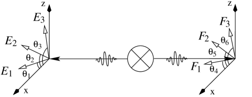
Figure 1: Measurements of $E_{1},E_{2},E_{3}$ on the “left,” and $F_{1},F_{2},F_{3}$ on the “right” hand side, along directions $\theta_{i}$.

Let us demonstrate the bounds on classical probabilities by the simplest nontrivial example of two propositions; e.g.,

$E\equiv$“a particle detector aligned along direction ${\bf a}$ clicks,” and
$F\equiv$“a particle detector aligned along direction ${\bf b}$ clicks.”

Consider also the joint proposition

$E\wedge F\equiv$ “the two particle detectors aligned along directions ${\bf a}$ and ${\bf b}$ click.”

The notation “1–1” alludes to the experimental setup, in which the two events are registered by detectors located at two “adjacent sites.” For multiple direction measurements, see Fig. 1.

There exist four possible cases, enumerated in Table 1(a).

   $\quad E\quad$ $\quad F\quad$ $\quad E\wedge F\equiv E\cdot F\quad$ $1$ 0 0 0 $2$ 0 1 0 $3$ 1 0 0 $4$ 1 1 1   full facet inequality $1$ $pq\geq 0$ $2$ $p\geq pq$ $3$ $p\geq pq$ $4$ $pq\geq p+q-1$ (a) (b)

Table 1: Construction of the correlation polytope for two events: (a) the four possible cases are represented by the truth table, whose rows can be interpreted as three-dimensional vectors forming the vertices of the correlation polytope; (b) the resulting four faces of the polytope are characterized by half-spaces which are obtained by solving the hull problem. .

The correlation polytope in this case is formed by interpreting the rows as vectors in three-dimensional vector space. Four cases, interpretable as truth assignments or two-valued measures, correspond to the four vectors $(0,0,0)$, $(0,1,0)$, $(1,0,0)$, and $(1,1,1)$. The correlation polytope for the probabilities $p$, $q$ and the joint probabilities $pq$ of an occurrence of $E$, $F$, and both $E\&F$

$$(p,q,pq)=\kappa_{1}(0,0,0)+\kappa_{2}(0,1,0)+\kappa_{3}(1,0,0)+\kappa_{4}(1,1,1)=(\kappa_{3}+\kappa_{4},\kappa_{2}+\kappa_{4},\kappa_{4})$$

is spanned by the convex sum $\kappa_{1}+\kappa_{2}+\kappa_{3}+\kappa_{4}=1$ of these four vectors, which thus are vertices of the polytope. $\kappa_{i}$ can be interpreted as the normalized weight for event $i$ to occur. The configuration is drawn in Figure 2.

1.5pt

Figure 2: The correlation polytope for two events. The vertices are $(0,0,0)$, $(0,1,0)$, $(1,0,0)$, and $(1,1,1)$. The four faces of the polytope are characterized by the inequalities in Table 1(b).

By the Minkoswki-Weyl representation theorem (e.g, Ref. [ziegler , p.29]), every convex polytope has a dual (equivalent) description: either as the convex hull of its extreme points (vertices); or as the intersection of a finite number of half-spaces. Such facets are given by linear inequalities, which are obtained from the set of vertices by solving the so called hull problem. The inequalities coincide with Boole’s “conditions of possible experience.” The hull problem is algorithmically solvable but computationally hard pit:90 .

In the above example, the “conditions of possible experience” are given by the inequalities enumerated in Table 1b). One of their consequences are bounds on joint occurrences of events. Suppose, for example, that the probability of a click in detector aligned along direction ${\bf a}$ is 0.9, and the probability of a click in the second detector aligned along direction ${\bf b}$ is 0.7. Then inequality 4 forces us to accept that the probability that both detector register clicks cannot be smaller than $0.9+0.7-1=0.6$. If, for instance, somebody comes up with a joint probability of $0.4$, we would know that this result is flawed, possibly by fundamental measurement errors, or by cheating, or by (quantum) “magic.”

II.3.2 Four-event “2–2” case

A configuration discussed in quantum mechanics is one with four events grouped into two equal parts $E_{1},E_{2}$ and $F_{1},F_{2}$. There are $2^{4}$ different cases of occurrence or nonoccurrence of these four events enumerated in Table 2.

$E_{1}$ $E_{2}$ $F_{1}$ $F_{2}$ $E_{1}F_{1}$ $E_{1}F_{2}$ $E_{2}F_{1}$ $E_{2}F_{2}$ 1 0 0 0 0 0 0 0 0 2 0 0 0 1 0 0 0 0 3 0 0 1 0 0 0 0 0 4 0 0 1 1 0 0 0 0 5 0 1 0 0 0 0 0 0 6 0 1 0 1 0 0 0 1 7 0 1 1 0 0 0 1 0 8 0 1 1 1 0 0 1 1 9 1 0 0 0 0 0 0 0 10 1 0 0 1 0 1 0 0 11 1 0 1 0 1 0 0 0 12 1 0 1 1 1 1 0 0 13 1 1 0 0 0 0 0 0 14 1 1 0 1 0 1 0 1 15 1 1 1 0 1 0 1 0 16 1 1 1 1 1 1 1 1

Table 2: Construction of the correlation polytope for four events. The 16 possible cases are represented by the truth table, whose rows can be interpreted as eight-dimensional vectors forming the vertices of the correlation polytope.

By solving the hull problem, one obtains a set of conditions of possible experience which represent the bounds on classical probabilities enumerated in Table 3. For historical reasons, the bounds 17-18, 19-20, 21-22, and 23-24 are called the Clauser-Horne inequalities cl-horne , clauser . They are equivalent (up to permutations of $p_{i},q_{i}$), and are the only additional inequalities structurally different from the two-event “1–1” case.

full facet inequality inequality for $p_{1}=p_{2}=q_{1}=q_{2}={1\over 2}$ 1 $p_{1}q_{1}\geq 0$ $p_{1}q_{1}\geq 0$ 2 $p_{1}q_{2}\geq 0$ $p_{1}q_{2}\geq 0$ 3 $p_{2}q_{1}\geq 0$ $p_{2}q_{1}\geq 0$ 4 $p_{2}q_{2}\geq 0$ $p_{2}q_{2}\geq 0$ 5 $p_{1}\geq p_{1}q_{1}$ ${1\over 2}\geq p_{1}q_{1}$ 6 $p_{1}\geq p_{1}q_{2}$ ${1\over 2}\geq p_{1}q_{2}$ 7 $q_{1}\geq p_{1}q_{1}$ ${1\over 2}\geq p_{1}q_{1}$ 8 $q_{1}\geq p_{1}q_{2}$ ${1\over 2}\geq p_{1}q_{2}$ 9 $p_{2}\geq p_{2}q_{1}$ ${1\over 2}\geq p_{2}q_{1}$ 10 $p_{2}\geq p_{2}q_{2}$ ${1\over 2}\geq p_{2}q_{2}$ 11 $q_{2}\geq p_{2}q_{1}$ ${1\over 2}\geq p_{2}q_{1}$ 12 $q_{2}\geq p_{1}q_{2}$ ${1\over 2}\geq p_{2}q_{2}$ 13 $p_{1}q_{1}\geq p_{1}+q_{1}-1$ $p_{1}q_{1}\geq 0$ 14 $p_{1}q_{2}\geq p_{1}+q_{2}-1$ $p_{1}q_{2}\geq 0$ 15 $p_{2}q_{1}\geq p_{2}+q_{1}-1$ $p_{2}q_{1}\geq 0$ 16 $p_{2}q_{2}\geq p_{2}+q_{2}-1$ $p_{2}q_{2}\geq 0$ 17 $0\geq p_{1}q_{1}+p_{1}q_{2}+p_{2}q_{1}-p_{2}q_{2}-p_{1}-q_{1}$ $1\geq+p_{1}q_{1}+p_{1}q_{2}+p_{2}q_{1}-p_{2}q_{2}$ 18 $p_{1}q_{1}+p_{1}q_{2}+p_{2}q_{1}-p_{2}q_{2}-p_{1}-q_{1}\geq-1$ $p_{1}q_{1}+p_{1}q_{2}+p_{2}q_{1}-p_{2}q_{2}\geq 0$ 19 $0\geq p_{1}q_{1}+p_{1}q_{2}-p_{2}q_{1}+p_{2}q_{2}-p_{1}-q_{2}$ $1\geq+p_{1}q_{1}+p_{1}q_{2}-p_{2}q_{1}+p_{2}q_{2}$ 20 $p_{1}q_{1}+p_{1}q_{2}-p_{2}q_{1}+p_{2}q_{2}-p_{1}-q_{2}\geq-1$ $p_{1}q_{1}+p_{1}q_{2}-p_{2}q_{1}+p_{2}q_{2}\geq 0$ 21 $0\geq p_{1}q_{1}-p_{1}q_{2}+p_{2}q_{1}+p_{2}q_{2}-p_{2}-q_{1}$ $1\geq p_{1}q_{1}-p_{1}q_{2}+p_{2}q_{1}+p_{2}q_{2}$ 22 $p_{1}q_{1}-p_{1}q_{2}+p_{2}q_{1}+p_{2}q_{2}-p_{2}-q_{1}\geq-1$ $p_{1}q_{1}-p_{1}q_{2}+p_{2}q_{1}+p_{2}q_{2}\geq 0$ 23 $0\geq-p_{1}q_{1}+p_{1}q_{2}+p_{2}q_{1}+p_{2}q_{2}-p_{2}-q_{2}$ $1\geq-p_{1}q_{1}+p_{1}q_{2}+p_{2}q_{1}+p_{2}q_{2}$ 24 $-p_{1}q_{1}+p_{1}q_{2}+p_{2}q_{1}+p_{2}q_{2}-p_{2}-q_{2}\geq-1$ $-p_{1}q_{1}+p_{1}q_{2}+p_{2}q_{1}-p_{2}q_{2}\geq 0$

Table 3: Construction of the correlation polytope for four events. The 24 faces of the polytope spanned by the vertices corresponding to the rows enumerated in Table 2. The bounds 17-18, 19-20, 21-22, and 23-24 are the Clauser-Horne inequalities.

II.3.3 Six event “3–3” case

A similar calculation 2000-poly for six events $E_{1},E_{2},E_{3},F_{1},F_{2},F_{3}$ depicted in Fig. 1 yields an additional independent collins-gisin-2003 , sliwa-2003 inequality for their probabilities $p_{1},p_{2},p_{3},q_{1},q_{2},q_{3}$ and their joint probabilities of the type

$$p_{1}q_{1}+p_{2}q_{2}+p_{1}q_{3}+p_{2}q_{1}+p_{2}q_{2}-p_{2}q_{3}+p_{3}q_{1}-p_{3}q_{2}\leq p_{1}+2q_{1}+q_{2}.$$

III Quantum contexts

Omniscience in a classical sense is no longer possible for quantum systems. Some of the reasons are: (i) quantum complementarity and, algebraically associated with it, the breakdown of distributivity; (ii) the impossibility to consistently assign truth and falsity for all observables simultaneously and, associated with it, the nonexistence of two-valued measures on even finite subsets of Hilbert logics; and (iii) the alleged randomness of certain single outcomes.

III.1 Hilbert lattices as quantum logics

Quantum logic has been introduced by Garrett Birkhoff and John von Neumann v-neumann-49 , birkhoff-36 , ma-57 , jauch , pulmannova-91 in the thirties. They organized it top-down, starting from the Hilbert space formalism of quantum mechanics. Certain entities of Hilbert spaces are identified with propositions, partial order relations and lattice operations. These relations and operations are identified with the logical implication relation and operations such as “and,” “or,” and the negation. Thereby, as we shall see, the resulting logical structures are “nonclassical,” in particular ”nonboolean.”

Kochen and Specker kochen2 , kochen3 suggested to consider only relations and operations among compatible, co-measurable observables; i.e., within Boolean subalgebras, which will be identified with blocks and contexts of Hilbert lattices. Nevertheless, some of their theorems formally take into account ensembles of contexts kochen1 for which a multitude of incompatible observables contribute.

If theoretical physics is assumed to be a faithful representation of our experience, such an “empirical,” “operational” bridgman27 , bridgman , bridgman52 logic derives its justification by the phenomena themselves. In this sense, one of the main justifications for quantum logic is the construction of the logical and algebraic order of events based on empirical findings.

III.1.1 Definition

The dimensionality of the Hilbert space for a given quantum system depends on the number of possible mutually exclusive outcomes. In the spin–${1\over 2}$ case, for example, there are two outcomes “up” and “down,” associated with spin state measurements along arbitrary directions. Thus, the dimensionality of Hilbert space needs to be two.

Then the following identifications can be made. Table 4 lists the identifications of relations of operations of classical Boolean set-theoretic and quantum Hillbert lattice types.

generic lattice	order relation	“meet”	“join”	“complement”
propositional	implication	disjunction	conjunction	negation
calculus	$\rightarrow$	“and” $\wedge$	“or” $\vee$	“not” $\neg$
“classical” lattice	subset $\subset$	intersection $\cap$	union $\cup$	complement
of subsets
of a set
Hilbert	subspace	intersection of	closure of	orthogonal
lattice	relation	subspaces $\cap$	linear	subspace
	$\subset$		span $\oplus$	$\perp$
lattice of	$E_{1}E_{2}=E_{1}$	$E_{1}E_{2}$	$E_{1}+E_{2}-E_{1}E_{2}$	orthogonal
commuting				projection
{noncommuting}		{$\displaystyle\lim_{n\rightarrow\infty}(E_{1}E_{2})^{n}$}
projection
operators

Table 4: Comparison of the identifications of lattice relations and operations for the lattices of subsets of a set, for experimental propositional calculi, for Hilbert lattices, and for lattices of commuting projection operators.

$\bullet$

Any closed linear subspace of — or, equivalently, any projection operator on — a Hilbert space corresponds to an elementary proposition. The elementary “true”–“false” proposition can in English be spelled out explicitly as

“The physical system has a property corresponding to the associated closed linear subspace.”

$\bullet$

The logical “and” operation is identified with the set theoretical intersection of two propositions “$\cap$”; i.e., with the intersection of two subspaces. It is denoted by the symbol “$\wedge$”. So, for two propositions $p$ and $q$ and their associated closed linear subspaces ${\mathfrak{M}}_{p}$ and ${\mathfrak{M}}_{q}$,

$${\mathfrak{M}}_{p\wedge q}=\{x\mid x\in{\mathfrak{M}}_{p},\;x\in{\mathfrak{M}}_{q}\}.$$

$\bullet$

The logical “or” operation is identified with the closure of the linear span “$\oplus$” of the subspaces corresponding to the two propositions. It is denoted by the symbol “$\vee$”. So, for two propositions $p$ and $q$ and their associated closed linear subspaces ${\mathfrak{M}}_{p}$ and ${\mathfrak{M}}_{q}$,

$${\mathfrak{M}}_{p\vee q}={\mathfrak{M}}_{p}\oplus{\mathfrak{M}}_{q}=\{x\mid x=\alpha y+\beta z,\;\alpha,\beta\in{\mathbb{C}},\;y\in{\mathfrak{M}}_{p},\;z\in{\mathfrak{M}}_{q}\}.$$

The symbol $\oplus$ will used to indicate the closed linear subspace spanned by two vectors. That is,

$$u\oplus v=\{w\mid w=\alpha u+\beta v,\;\alpha,\beta\in{\mathbb{C}},\;u,v\in{\mathfrak{H}}\}.$$

Notice that a vector of Hilbert space may be an element of ${\mathfrak{M}}_{p}\oplus{\mathfrak{M}}_{q}$ without being an element of either ${\mathfrak{M}}_{p}$ or ${\mathfrak{M}}_{q}$, since ${\mathfrak{M}}_{p}\oplus{\mathfrak{M}}_{q}$ includes all the vectors in ${\mathfrak{M}}_{p}\cup{\mathfrak{M}}_{q}$, as well as all of their linear combinations (superpositions) and their limit vectors.

$\bullet$

The logical “not”-operation, or “negation” or “complement,” is identified with operation of taking the orthogonal subspace “$\perp$”. It is denoted by the symbol “ ^′ ”. In particular, for a proposition $p$ and its associated closed linear subspace ${\mathfrak{M}}_{p}$, the negation $p^{\prime}$ is associated with

$${\mathfrak{M}}_{p^{\prime}}=\{x\mid(x,y)=0,\;y\in{\mathfrak{M}}_{p}\},$$

where $(x,y)$ denotes the scalar product of $x$ and $y$.

$\bullet$

The logical “implication” relation is identified with the set theoretical subset relation “$\subset$”. It is denoted by the symbol “$\rightarrow$”. So, for two propositions $p$ and $q$ and their associated closed linear subspaces ${\mathfrak{M}}_{p}$ and ${\mathfrak{M}}_{q}$,

$${p\rightarrow q}\Longleftrightarrow{\mathfrak{M}}_{p}\subset{\mathfrak{M}}_{q}.$$

$\bullet$

A trivial statement which is always “true” is denoted by $1$. It is represented by the entire Hilbert space $\mathfrak{H}$. So,

$${\mathfrak{M}}_{1}=\mathfrak{H}.$$

$\bullet$

An absurd statement which is always “false” is denoted by $0$. It is represented by the zero vector $0$. So,

$${\mathfrak{M}}_{0}=0.$$

III.1.2 Diagrammatical representation, blocks, complementarity

Propositional structures are often represented by Hasse and Greechie diagrams. A Hasse diagram is a convenient representation of the logical implication, as well as of the “and” and “or” operations among propositions. Points “ $\bullet$ ” represent propositions. Propositions which are implied by other ones are drawn higher than the other ones. Two propositions are connected by a line if one implies the other. Atoms are propositions which “cover” the least element $0$; i.e., they lie “just above” $0$ in a Hasse diagram of the partial order.

A much more compact representation of the propositional calculus can be given in terms of its Greechie diagram greechie:71 . In this representation, the emphasis is on Boolean subalgebras. Points “ $\circ$ ” represent the atoms. If they belong to the same Boolean subalgebra, they are connected by edges or smooth curves. The collection of all atoms and elements belonging to the same Boolean subalgebra is called block; i.e., every block represents a Boolean subalgebra within a nonboolean structure. The blocks can be joined or pasted together as follows.

$\bullet$

The tautologies of all blocks are identified.

$\bullet$

The absurdities of all blocks are identified.

$\bullet$

Identical elements in different blocks are identified.

$\bullet$

The logical and algebraic structures of all blocks remain intact.

This construction is often referred to as pasting construction. If the blocks are only pasted together at the tautology and the absurdity, one calls the resulting logic a horizontal sum.

Every single block represents some “maximal collection of co-measurable observables” which will be identified with some quantum context. Hilbert lattices can be thought of as the pasting of a continuity of such blocks or contexts.

Note that whereas all propositions within a given block or context are co-measurable; propositions belonging to different blocks are not. This latter feature is an expression of complementarity. Thus from a strictly operational point of view, it makes no sense to speak of the “real physical existence” of different contexts, as knowledge of a single context makes impossible the measurement of all the other ones.

Einstein-Podolski-Rosen (EPR) type arguments epr utilizing a configuration sketched in Fig. 1 claim to be able to infer two different contexts counterfactually. One context is measured on one side of the setup, the other context on the other side of it. By the uniqueness property svozil-2004-vax , svozil-2006-uniquenessprinciple of certain two-particle states, knowledge of a property of one particle entails the certainty that, if this property were measured on the other particle as well, the outcome of the measurement would be a unique function of the outcome of the measurement performed. This makes possible the measurement of one context, as well as the simultaneous counterfactual inference of another, mutual exclusive, context. Because, one could argue, although one has actually measured on one side a different, incompatible context compared to the context measured on the other side, if on both sides the same context would be measured, the outcomes on both sides would be uniquely correlated. Hence measurement of one context per side is sufficient, for the outcome could be counterfactually inferred on the other side.

As problematic as counterfactual physical reasoning may appear from an operational point of view even for a two particle state, the simultaneous “counterfactual inference” of three or more blocks or contexts fails because of the missing uniqueness property svozil-2006-uniquenessprinciple of quantum states.

As a first example, we shall paste together observables of the spin one-half systems. We have associated a propositional system

$$L({\bf a})=\{0,E,E^{\prime},1\},$$

corresponding to the outcomes of a measurement of the spin states along some arbitrary direction ${\bf a}$. If the spin states would be measured along a different spatial direction, say ${\bf b}\neq\pm{\bf a}$, an identical propositional system

$$L({\bf b})=\{0,F,F^{\prime},1\}$$

would have resulted, with the propositions $E$ and $F$ explicitly expressed before. The two-dimensional Hilbert space representation of this configuration is depicted in Figure 3.

1.5pt

Figure 3: Two-dimensional configuration of spin $1/2$ state measurements along two directions ${\bf a}$ and ${\bf b}$.

$L({\bf a})$ and $L({\bf b})$ can be joined by pasting them together. In particular, we identify their tautologies and absurdities; i.e., $0$ and $1$. All the other propositions remain distinct. We then obtain a propositional structure

$$L({\bf a})\oplus L({\bf b})=MO_{2}$$

whose Hasse diagram is of the “Chinese lantern” form and is drawn in Figure 4(a). The corresponding Greechie Diagram is drawn in Figure 4(b). Here, the “$O$” stands for orthocomplementation, expressing the fact that for every element there exists an orthogonal complement. The term “$M$” stands for modularity; i.e., for all $x\rightarrow b$, $x\vee(a\wedge b)=(x\vee a)\wedge b$. The subscript “2” stands for the pasting of two Boolean subalgebras $2^{2}$. Since all possible directions ${\bf a}\in{\mathbb{R}}^{3}$ form a continuum, the Hilbert lattice is a continuum of pastings of subalgebras of the form $L({\bf a})$.

1.5pt		1.5pt
(a)		(b)

Figure 4: (a) Hasse diagram of the “Chinese lantern” form obtained by the pasting of two spin one-half propositional systems $L(x)$ and $L(\overline{x})$ which are nonco-measurable. The resulting logical structure is a modular orthocomplemented lattice $L(x)\oplus L(\overline{x})=MO_{2}$. The blocks (without $0,1$) are indicated by dashed boxes. (b) Greechie diagram of the configuration depicted in (a).

The propositional system obtained is not a classical Boolean algebra, since the distributive laws are not satisfied; i.e.,

$$\begin{array}[b]{ccc}F\vee(E\wedge E^{\prime})&\stackrel{{\scriptstyle?}}{{=}}&(F\vee E)\wedge(F\vee E^{\prime})\\ F\vee 0&\stackrel{{\scriptstyle?}}{{=}}&1\wedge 1\\ F&\neq&1,\end{array}$$

$$\begin{array}[b]{ccc}F\wedge(E\vee E^{\prime})&\stackrel{{\scriptstyle?}}{{=}}&(F\wedge E)\vee(F\wedge E^{\prime})\\ F\wedge 1&\stackrel{{\scriptstyle?}}{{=}}&0\vee 0\\ F&\neq&0.\end{array}$$

Notice that the expressions can be easily evaluated by using the Hasse diagram 4(a): For any $a,b$, $a\vee b$ is just the least element which is connected by $a$ and $b$; $a\wedge b$ is just the highest element connected to $a$ and $b$. Intermediates which are not connected to both $a$ and $b$ do not count. That is,

1pt

$a\vee b$ is called a least upper bound of $a$ and $b$. $a\wedge b$ is called a greatest lower bound of $a$ and $b$.

$MO_{2}$ is a specific example of an algebraic structure which is called a lattice. Any two elements of a lattice have a least upper and a greatest lower bound satisfying the commutative, associative and absorption laws.

Nondistributivity is the algebraic expression of nonclassicality, but what is the algebraic reason for nondistributivity? It is, heuristically speaking, scarcity, the lack of necessary algebraic elements to “fill up” all propositions necessary to obtain one and the same result in both ways as expressed by the distributive law.

III.2 Quantum contexts as blocks

All that is operationally knowable for a given quantized system is a single block representing co-measurable observables. Thus, single blocks or, in another terminology, maximal Boolean subalgebras of Hilbert lattices, will be identified with quantum contexts. As Hilbert lattices are pastings of a continuity of blocks or contexts, contexts are the building blocks of quantum logics.

A quantum context can equivalently be formalized by a single (nondegenerate) “maximal” self-adjoint operator $C$, such that all commuting, compatible co-measurable observables are functions thereof. (e.g., Ref. v-neumann-49 , Sec. II.10, p. 90, English translation p. 173; Ref. kochen1 , § 2; Ref. neumark-54 , pp. 227,228; Ref. halmos-vs , § 84). Note that mutually commuting opators have identical pairwise orthogonal sets of eigenvectors (forming an orthonormal basis) which correspond to pairwise orthogonal projectors adding up to unity. The spectral decompositions of the mutually commuting opators thus contain sums of identical pairwise orthogonal projectors.

Thus the “maximal” self-adjoint operator ${C}$ has a spectral decomposition into some complete set of orthogonal projectors ${E}_{i}$ which correspond to elementary “yes”-“no” propositions in the Von Neumann-Birkhoff type sense v-neumann-49 , birkhoff-36 . That is, ${C}=\sum_{i=1}^{n}c_{i}{E}_{i}$ with mutually different $c_{i}$ and $\sum_{i=1}^{n}{E}_{i}={\mathbb{I}}$. In $n$ dimensions, contexts can be viewed as $n$-pods spanned by the $n$ orthogonal vectors corresponding to the projectors ${E}_{1},{E}_{2},\cdots,{E}_{n}$. As there exist many such representations with many different sets of coefficients $c_{i}$, “maximal” operator are not unique.

An observable belonging to two or more contexts is called link observable. Contexts can thus be depicted by Greechie diagrams greechie:71 , consisting of points which symbolize observables (representable by the spans of vectors in $n$-dimensional Hilbert space). Any $n$ points belonging to a context; i.e., to a maximal set of co-measurable observables (representable as some orthonormal basis of $n$-dimensional Hilbert space), are connected by smooth curves. Two smooth curves may be crossing in common link observables. In three dimensions, smooth curves and the associated points stand for tripods. Still another compact representation is in terms of Tkadlec diagrams tkadlec-00 , in which points represent complete tripods and smooth curves represent single legs interconnecting them.

In two dimensional Hilbert space, interlinked contexts do not exist, since every context is fixed by the assumption of one property. The entire context is just this property, together with its negation, which corresponds to the orthogonal ray (which spans a one dimensional subspace) or projection associated with the ray corresponding to the property.

The simplest nontrivial configuration of interlinked contexts exists in three-dimensional Hilbert space. Consider an arrangement of five observables $A$, $B$, $C$, $D$, $K$ with two systems of operators $\{A,B,C\}$ and $\{D,K,A\}$, the contexts, which are interconnected by $A$. Within a context, the operators commute and the associated observables are co-measurable. For two different contexts, operators outside the link operators do not commute. $A$ is a link observable. This propositional structure (also known as $L_{12}$) can be represented in three-dimensional Hilbert space by two tripods with a single common leg. Fig. 5 depicts this configuration in three-dimensional real vector space, as well as in the associated Greechie and Tkadlec diagrams.

1.5pt		2pt		2pt
(a)		(b)		(c)

Figure 5: Three equivalent representations of the same geometric configuration: (a) Two tripods with a common leg; (b) Greechie (orthogonality) diagram: points stand for individual basis vectors, and orthogonal tripods are drawn as smooth curves; (c) Tkadlec diagram: points represent complete tripods and smooth curves represent single legs interconnecting them.

The operators $B,C,A$ and $D,K,A$ can be identified with the projectors corresponding to the two bases

$$\begin{array}[]{lcl}B_{B-C-A}&=&\{(1,0,0)^{T},(0,1,0)^{T},(0,0,1)^{T}\},\\ B_{D-K-A}&=&\{(\cos\varphi,\sin\varphi,0)^{T},(-\sin\varphi,\cos\varphi,0)^{T},(0,0,1)^{T}\},\end{array}$$

(the superscript “$T$” indicates transposition). Their matrix representation is the dyadic product of every vector with itself.

Physically, the union of contexts $\{B,C,A\}$ and $\{D,K,A\}$ interlinked along $A$ does not have any direct operational meaning; only a single context can be measured along a single quantum at a time; the other being irretrievably lost if no reconstruction of the original state is possible. Thus, in a direct way, testing the value of observable $A$ against different contexts $\{B,C,A\}$ and $\{D,K,A\}$ is metaphysical.

It is, however, possible to counterfactually retrieve information about the two different contexts of a single quantum indirectly by considering a singlet state $|\Psi_{2}\rangle=({1/\sqrt{3}})(|+-\rangle+|-+\rangle-|00\rangle)$ via the “explosion view” Einstein-Podolsky-Rosen type of argument depicted in Fig. 1. Since the state is form invariant with respect to variations of the measurement angle and at the same time satisfies the uniqueness property svozil-2006-uniquenessprinciple , one may retrieve the first context $\{B,C,A\}$ from the first quantum and the second context $\{D,K,A\}$ from the second quantum. (This is a standard procedure in Bell type arguments with two spin one-half quanta.)

More tightly interlinked contexts such as $\{A,B,C\}-\{C,D,E\}-\{E,F,A\}$, whose Greechie diagram is a triangle with the edges $A$, $C$ and $E$, or $\{A,B,C\}-\{C,D,E\}-\{E,F,G\}-\{G,H,A\}$, whose Greechie diagram is a quadrangle with the edges $A$, $C$, $E$ and $G$, cannot be represented in Hilbert space and thus have no realization in quantum logics. The five contexts $\{A,B,C\}-\{C,D,E\}-\{E,F,G\}-\{G,H,I\}-\{I,J,A\}$ whose Greechie diagrams is a pentagon with the edges $A$, $C$, $E$, $G$ and $I$ have realizations in ${\mathbb{R}}^{3}$ svozil-tkadlec .

III.3 Probability theory

III.3.1 Kochen-Specker theorem

Quantum logics of Hilbert space dimension greater than two have not a single two-valued state interpretable as consistent, overall truth assignment specker-60 . This is the gist of the beautiful construction of Kochen and Specker kochen1 . For similar theorems, see Refs. ZirlSchl-65 , Alda , Alda2 , kamber64 , kamber65 . As a result of the nonexistence of two-valued states, the classical strategy to construct probabilities by a convex combination of all two-valued states fails entirely.

One of the most compact and comprehensive versions of the Kochen-Specker proof by contradiction in three-dimensional Hilbert space ${\mathbb{R}}^{3}$ has been given by Peres peres-91 . (For other discussions, see Refs. stairs83 , redhead , jammer-92 , brown , peres-91 , peres , penrose-ks , clifton-93 , mermin-93 , svozil-tkadlec .) Peres’ version uses a 33-element set of lines without a two-valued state. The direction vectors of these lines arise by all permutations of coordinates from

$$(0,0,1),\;(0,\pm 1,1),\;(0,\pm 1,\sqrt{2}),\;\;\textrm{ and }\;(\pm 1,\pm 1,\sqrt{2}).$$

These lines can be generated (by the “nor”-operation between nonorthogonal propositions) by the three lines svozil-tkadlec

$$(1,0,0),\;(1,1,0),\;(\sqrt{2},1,1).$$

Note that as three arbitrary but mutually nonorthogonal lines generate a dense set of lines havlicek , it can be expected that any such triple of lines (not just the one explicitly mentioned) generates a finite set of lines which does not allow a two-valued probability measure.

The way it is defined, this set of lines is invariant under interchanges (permutations) of the $x_{1},x_{2}$ and $x_{3}$ axes, and under a reversal of the direction of each of these axes. This symmetry property allows us to assign the probability measure $1$ to some of the rays without loss of generality. Assignment of probability measure $0$ to these rays would be equivalent to renaming the axes, or reversing one of the axes.

The Greechie diagram of the Peres configuration is given in Figure 6 svozil-tkadlec . For simplicity, 24 points which belong to exactly one edge are omitted. The coordinates should be read as follows: $\bar{1}\rightarrow-1$ and $2\rightarrow\sqrt{2}$; e.g., 1$\bar{1}$2 denotes $\textrm{Sp}(1,-1,\sqrt{2})$. Concentric circles indicate the (non orthogonal) generators mentioned above.

Figure 6: Greechie diagram of a finite subset of the continuum of blocks or contexts embeddable in three-dimensional real Hilbert space without a two-valued probability measure [svozil-tkadlec , Figure 9].

Let us prove that there is no two-valued probability measure svozil-tkadlec , tkadlec-96 . Due to the symmetry of the problem, we can choose a particular coordinate axis such that, without loss of generality, $P(100)=1$. Furthermore, we may assume (case 1) that $P(21\bar{1})=1$. It immediately follows that $P(001)=P(010)=P(102)=P(\bar{1}20)=0$. A second glance shows that $P(20\bar{1})=1$, $P(1\bar{1}2)=P(112)=0$.

Let us now suppose (case 1a) that $P(201)=1$. Then we obtain $P(\bar{1}12)=P(\bar{1}\bar{1}2)=0$. We are forced to accept $P(110)=P(1\bar{1}0)=1$ — a contradiction, since $(110)$ and $(1\bar{1}0)$ are orthogonal to each other and lie on one edge.

Hence we have to assume (case 1b) that $P(201)=0$. This gives immediately $P(\bar{1}02)=1$ and $P(211)=0$. Since $P(01\bar{1})=0$, we obtain $P(2\bar{1}\bar{1})=1$ and thus $P(120)=0$. This requires $P(2\bar{1}0)=1$ and therefore $P(12\bar{1})=P(121)=0$. Observe that $P(210)=1$, and thus $P(\bar{1}2\bar{1})=P(\bar{1}21)=0$. In the following step, we notice that $P(10\bar{1})=P(101)=1$ — a contradiction, since $(101)$ and $(10\bar{1})$ are orthogonal to each other and lie on one edge.

Thus we are forced to assume (case 2) that $P(2\bar{1}1)=1$. There is no third alternative, since $P(011)=0$ due to the orthogonality with $(100)$. Now we can repeat the argument for case 1 in its mirrored form.

The most compact way of deriving the Kochen-Specker theorem in four dimensions has been given by Cabello cabello-96 , cabello-99 . It is depicted in Fig. 7.

2pt	2pt
(a)	(b)

Figure 7: Greechie diagram of a finite subset of the continuum of blocks or contexts embeddable in four-dimensional real Hilbert space without a two-valued probability measure cabello-96 , cabello-99 . The proof of the Kochen-Specker theorem uses nine tightly interconnected contexts $\color[rgb]{0,0,1}a=\{A,B,C,D\}$, $\color[rgb]{1,0,0}b=\{D,E,F,G\}$, $\color[rgb]{0,1,0}c=\{G,H,I,J\}$, $\color[rgb]{.5,0,.5}d=\{J,K,L,M\}$, $\color[rgb]{1,1,0}e=\{M,N,O,P\}$, $\color[rgb]{1,0,1}f=\{P,Q,R,A\}$, $\color[rgb]{1,.5,0}g=\{B,I,K,R\}$, $\color[rgb]{0.5,0.5,0}h=\{C,E,L,N\}$, $\color[rgb]{0,1,1}i=\{F,H,O,Q\}$ consisting of the 18 projectors associated with the one dimensional subspaces spanned by $A=(0,0,1,-1)$, $B=(1,-1,0,0)$, $C=(1,1,-1,-1)$, $D=(1,1,1,1)$, $E=(1,-1,1,-1)$, $F=(1,0,-1,0)$, $G=(0,1,0,-1)$, $H=(1,0,1,0)$, $I=(1,1,-1,1)$, $J=(-1,1,1,1)$, $K=(1,1,1,-1)$, $L=(1,0,0,1)$, $M=(0,1,-1,0)$, $N=(0,1,1,0)$, $O=(0,0,0,1)$, $P=(1,0,0,0)$, $Q=(0,1,0,0)$, $R=(0,0,1,1)$. (a) Greechie diagram representing atoms by points, and contexts by maximal smooth, unbroken curves. (b) Dual Tkadlec diagram representing contexts by filled points, and interconnected contexts are connected by lines. (Duality means that points represent blocks and maximal smooth curves represent atoms.) Every observable proposition occurs in exactly two contexts. Thus, in an enumeration of the four observable propositions of each of the nine contexts, there appears to be an even number of true propositions. Yet, as there is an odd number of contexts, there should be an odd number (actually nine) of true propositions.

III.3.2 Gleason’s derivation of the Born rule

In view of the nonexistence of classical two-valued states on even finite superstructures of blocks or contexts associated with quantized systems, one could still resort to classicality within blocks or contexts. According to Gleason’s theorem, this is exactly the route, the “via regia,” to the quantum probabilities, in particular to the Born rule.

According to the Born rule, the expectation value $\langle A\rangle$ of an observable $A$ is the trace of $\rho A$; i.e., $\langle A\rangle={\rm tr}(\rho A)$. In particular, if $A$ is a projector $E$ corresponding to an elementary yes-no proposition “the system has property Q,” then $\langle E\rangle={\rm tr}(\rho E)$ corresponds to the probability of that property $Q$ if the system is in state $\rho$. The equations $\rho^{2}=\rho$ and ${\rm tr}(\rho^{2})=1$ are only valid for pure states, because $\rho$ is not an projector and thus idempotent for mixed states.

It is still possible to ascribe a certain degree of classical probabilistic behaviour to a quantum logic by considering its block superstructure. Due to their Boolean algebra, blocks are “classical mini-universes.” It is one of the mindboggling features of quantum logic that it can be decomposed into a pasting of blocks. Conversely, by a proper arrangement of “classical mini-universes,” quantum Hilbert logics can be obtained. This theme is used in quantum probability theory, in particular by the Gleason and the Kochen-Specker theorems. In this sense, Gleason’s theorem can be understood as the functional analytic generalization of the generation of all classical probability distributions by a convex sum of the extreme cases.

Gleason’s theorem Gleason , r:dvur-93 , c-k-m , peres , hru-pit-2003 , rich-bridge is a derivation of the Born rule from fundamental assumptions about quantum probabilities, guided by the quasi–classical; i.e., Boolean, sub-parts of quantum theory. Essentially, the main assumption required for Gleason’s theorem is that within blocks or contexts, the quantum probabilities behave as classical probabilities; in particular the sum of probabilities over a complete set of mutually exclusive events add up to unity. With these quasi–classical provisos, Gleason proved that there is no alternative to the Born rule for Hilbert spaces of dimension greater than two.

III.4 Quantum violations of classical probability bounds

Due to the different form of quantum correlations, which formally is a consequence of the different way of defining quantum probabilities, the constraints on classical probabilities are violated by quantum probabilities. Quantitatively, this can be investigated filipp-svo-04-qpoly-prl by substituting the classical probabilities by the quantum ones; i.e.,

$$\begin{array}[]{lll}p_{1}&\rightarrow&q_{1}(\theta)={\frac{1}{2}}\left[{\mathbb{I}}_{2}+{\bf\sigma}(\theta)\right]\otimes{\mathbb{I}}_{2},\\ p_{3}&\rightarrow&q_{3}(\theta)={\mathbb{I}}_{2}\otimes{\frac{1}{2}}\left[{\mathbb{I}}_{2}+{\bf\sigma}(\theta)\right],\\ p_{ij}&\rightarrow&q_{ij}(\theta,\theta^{\prime})={\frac{1}{2}}\left[{\mathbb{I}}_{2}+{\bf\sigma}(\theta)\right]\otimes{\frac{1}{2}}\left[{\mathbb{I}}_{2}+{\bf\sigma}(\theta^{\prime})\right],\end{array}$$

with ${\bf\sigma}(\theta)=\left(\begin{array}[]{ll}\cos\theta&\sin\theta\\ \sin\theta&-\cos\theta\end{array}\right)$, where $\theta$ is the relative measurement angle in the $x$–$z$-plane, and the two particles propagate along the $y$-axis, as depicted in Fig. 1.

The quantum transformation associated with the Clauser-Horne inequality for the 2–2 case is given by

$$\begin{array}[]{lcl}O_{22}(\alpha,\beta,\gamma,\delta)&=&q_{13}(\alpha,\gamma)+q_{14}(\alpha,\delta)+q_{23}(\beta,\gamma)-q_{24}(\beta,\delta)-q_{1}(\alpha)-q_{3}(\gamma)\\ &=&{\frac{1}{2}}\left[{\mathbb{I}}_{2}+{\bf\sigma}(\alpha)\right]\otimes{\frac{1}{2}}\left[{\mathbb{I}}_{2}+{\bf\sigma}(\gamma)\right]+{\frac{1}{2}}\left[{\mathbb{I}}_{2}+{\bf\sigma}(\alpha)\right]\otimes{\frac{1}{2}}\left[{\mathbb{I}}_{2}+{\bf\sigma}(\delta)\right]\\ &&+{\frac{1}{2}}\left[{\mathbb{I}}_{2}+{\bf\sigma}(\beta)\right]\otimes{\frac{1}{2}}\left[{\mathbb{I}}_{2}+{\bf\sigma}(\gamma)\right]-{\frac{1}{2}}\left[{\mathbb{I}}_{2}+{\bf\sigma}(\beta)\right]\otimes{\frac{1}{2}}\left[{\mathbb{I}}_{2}+{\bf\sigma}(\delta)\right]\\ &&-{\frac{1}{2}}\left[{\mathbb{I}}_{2}+{\bf\sigma}(\alpha)\right]\otimes{\mathbb{I}}_{2}-{\mathbb{I}}_{2}\otimes{\frac{1}{2}}\left[{\mathbb{I}}_{2}+{\bf\sigma}(\gamma)\right],\end{array}$$

where $\alpha$, $\beta$, $\gamma$, $\delta$ denote the measurement angles lying in the $x$–$z$-plane: $\alpha$ and $\beta$ for one particle, $\gamma$ and $\delta$ for the other one. The eigenvalues are

$$\lambda_{1,2,3,4}(\alpha,\beta,\gamma,\delta)=\frac{1}{2}\big{(}\pm\sqrt{1\pm\sin(\alpha-\beta)\sin(\gamma-\delta)}-1\big{)}$$

yielding the maximum bound $\|O_{22}\|=\max_{i=1,2,3,4}\lambda_{i}$. Note that for the particular choice of parameters $\alpha=0,\beta=2\theta,\gamma=\theta,\delta=3\theta$ adopted in cabello-2003a , filipp-svo-04-qpoly , one obtains $|O_{22}|=\frac{1}{2}\left\{\left[\left(3-\cos 4\theta\right)/2\right]^{1/2}-1\right\}\leq\frac{1}{2}\left(\sqrt{2}-1\right)$, as compared to the classically allowed bound from above $0$.

III.5 Interpretations

The nonexistence of two-valued states on the set of quantum propositions (of greater than two-dimensional Hilbert spaces) interpretable as truth assignments poses a great challenge for the interpretation of quantum logical propositions, relations and operations, as well as for quantum mechanics in general. At stake is the meaning and physical co-existence of observables which are not co-measurable. Several interpretations have been proposed, among them contextuality, as well as the abandonment of classical omniscience and realism discussed below.

III.5.1 Contextuality

Contextuality abandons the context independence of measurement outcomes bell-66 , hey-red , redhead by supposing that it is wrong to assume (cf. Ref. bell-66 , Sec. 5) that the result of an observation is independent of what observables are measured alongside of it. Bell [bell-66 , Sec. 5] states that the

“$\ldots$ result of an observation may reasonably depend not only on the state of the system $\ldots$ but also on the complete disposition of the apparatus.”

Note also Bohr’s remarks bohr-1949 about

“the impossibility of any sharp separation between the behavior of atomic objects and the interaction with the measuring instruments which serve to define the conditions under which the phenomena appear.”

Contextuality might be criticized as an attempt to maintain omniscience and omni-realism even in view of a lack of consistently assignable truth values on quantum propositions. Omniscience or omni-realism is the belief that

“all observables exist even without being experienced by any finite mind.”

Contextuality supposes that an

“observable exists without being experienced by any finite mind, but it may have different values, depending on its context.”

So far, despite some claims to have measured contextuality, there is no direct experimental evidence. Some experimental findings inspired by Bell-type inequalities aspect-81 , aspect-82a , wjswz-98 , the Kochen-Specker theorem simon-2002 , hasegawa:230401 as well as the Greenberger-Horne-Zeilinger theorem panbdwz measure incompatible contexts one after another; i.e., temporally sequentially, and not simultaneously. Hence, different contexts can only be measured on different particles. A more direct test of contextuality might be an EPR configuration of two quanta in three-dimensional Hilbert space interlinked in a single observable, as discussed above.

III.5.2 Abandonment of classical omniscience

As has been pointed out already, contextuality might be criticized for its presumption of quantum omniscience; in particular the supposition that a physical system, at least in principle, is capable of “carrying” all answers to any classically retrievable question. This is true classically, since the classical context is the entirety of observables. But it need not be true for other types of (finite) systems or agents. Take for example, a refrigerator. If it is automated in a way to tell you whether or not there is enough milk in it, it will be at a complete loss at answering a totally different question, such as if there is enough oil in the engine of your car. It is a matter of everday experience that not all agents are prepared to give answers to all perceivable questions.

Nevertheless, if one forces an agent to answer a question it is incapable to answer, the agent might throw some sort of “fair coin” — if it is capable of doing so — and present random answers. This scenario of a context mismatch between preparation and measurement is the basis of quantum random number generators Quantis which serve as a kind of “quantum random oracle” Cris04 , calude-dinneen05 . It should be kept in mind that randomness, at least algorithmically chaitin2 , chaitin3 , calude:02 , does not come “for free,” thus exhibiting an amazing capacity of single quanta to support random outcomes. Alternatively, the unpredictable, erratic outcomes might, in the context translation svozil-2003-garda scenario, be due to some stochasticity originating from the interaction with a “macroscopic” measurement apparatus, and the undefined.

One interpretation of the impossibility to operationalize more than a single context is the abandonment of classical omniscience: in this view, whereas it might be meaningful theoretically and formally to study the entirety of the context superstructure, only a single context operationally exists. Note that, in a similar way as retrieving information from a quantized system, the only information codable into a quantized system is given by a single block or context. If the block contains $n$ atoms corresponding to $n$ possible measurement outcomes, then the information content is a $n$it zeil-99 , DonSvo01 , svozil-2002-statepart-prl . The information needs not be “located” at a particular particle, as it can be “distributed” over a multi–partite state. In this sense, the quantum system could be viewed as a kind of (possibly nonlocal) programmable integrated circuit, such as a field programmable qate array or an application specific integrated circuit.

Quantum observables make only sense when interpreted as a function of some context, formalized by either some Boolean subalgebra or by the maximal operator. It is useless in this framework to believe in the existence of a single isolated observable devoid of the context from which it is derived. In this holistic approach, isolated observables separated from its missing contexts do not exist.

Likwise, it is wrong to assume that all observables which could in principle (“potentially”) have been measured, also co-exist, irrespective of whether or not they have or could have been actually measured. Realism in the sense of

“co-measurable entities sometimes exist without being experienced by any finite mind” might still be assumed for a single context, in particular the one in which the system was prepared.

III.5.3 Subjective idealism

Still another option is subjective idealism, denying the “existence” of observables which could in principle (“potentially”) have been measured, but actually have not been measured: in this view, it is wrong to assume that stace

“entities sometimes exist without being experienced by any finite mind.”

Indeed, Bekeley states berkeley ,

“For as to what is said of the absolute existence of unthinking things without any relation to their being perceived, that seems perfectly unintelligible. Their esse [[to be]] is percepi [[to be perceived]], nor is it possible they should have any existence out of the minds or thinking things which perceive them.”

With this assumption, the Bell, Kochen-Specker and Greenberger-Horne-Zeilinger theorems and similar have merely theoretical, formal relevance for physics, because they operate with unobservable physical “observables” and entities or with counterfactuals which are inferred rather than measured.

IV Automata and generalized urn logic

The following quasi–classical logics take up the notion of contexts as blocks representing Boolean subalgebras and the pastings among them. They are quasi–classical, because unlike quantum logics they possess sufficiently many two-valued states to allow embeddings into Boolean algebras.

IV.1 Partition logic

The empirical logics (i.e., the propositional calculi) associated with the generalized urn models suggested by Ron Wright wright:pent , wright , and automaton logics (APL) svozil-93 , schaller-96 , dvur-pul-svo , cal-sv-yu , svozil-ql are equivalent (cf. Refs. [svozil-ql , p.145] and svozil-2001-eua ) and can be subsumed by partition logics. The logical equivalence of automaton models with generalized urn models suggests that these logics are more general and “robust” with respect to changes of the particular model than could have been expected from the particular instances of their first appearance.

Again the concept of context or block is very important here. Partition logics are formed by pasting together contexts or blocks based on the partitions of a set of states. The contexts themselves are derived from the input/output analysis of experiments.

IV.2 Generalized urn models

A generalized urn model ${\cal U}=\langle U,C,L,\Lambda\rangle$ is characterized as follows. Consider an ensemble of balls with black background color. Printed on these balls are some color symbols from a symbolic alphabet $L$. The colors are elements of a set of colors $C$. A particular ball type is associated with a unique combination of mono-spectrally (no mixture of wavelength) colored symbols printed on the black ball background. Let $U$ be the set of ball types. We shall assume that every ball contains just one single symbol per color. (Not all types of balls; i.e., not all color/symbol combinations, may be present in the ensemble, though.)

Let $|U|$ be the number of different types of balls, $|C|$ be the number of different mono-spectral colors, $|L|$ be the number of different output symbols.

Consider the deterministic “output” or “lookup” function $\Lambda(u,c)=v$, $u\in U$, $c\in C$, $v\in L$, which returns one symbol per ball type and color. One interpretation of this lookup function $\Lambda$ is as follows. Consider a set of $|C|$ eyeglasses build from filters for the $|C|$ different colors. Let us assume that these mono-spectral filters are “perfect” in that they totally absorb light of all other colors but a particular single one. In that way, every color can be associated with a particular eyeglass and vice versa.

When a spectator looks at a particular ball through such an eyeglass, the only operationally recognizable symbol will be the one in the particular color which is transmitted through the eyeglass. All other colors are absorbed, and the symbols printed in them will appear black and therefore cannot be differentiated from the black background. Hence the ball appears to carry a different “message” or symbol, depending on the color at which it is viewed. This kind of “complementarity” has been used for a demonstration of quantum cryptography svozil-2005-ln1e .

An empirical logic can be constructed as follows. Consider the set of all ball types. With respect to a particular colored eyeglass, this set disjointly “decays” or gets partitioned into those ball types which can be separated by the particular color of the eyeglass. Every such partition of ball types can then be identified with a Boolean algebra whose atoms are the elements of the partition. A pasting of all of these Boolean algebras yields the empirical logic associated with the particular urn model.

Consider, for the sake of demonstration, a single color and its associated partition of the set of ball types (ball types within a given element of the partition cannot be differetiated by that color). In the generalized urn model, an element $a$ of this partition is a set of ball types which corresponds to an elementary proposition

“the ball drawn from the urn is of the type contained in $a$.”

IV.3 Automaton models

A (Mealy type) automaton ${\cal A}=\langle S,I,O,\delta,\lambda\rangle$ is characterized by the set of states $S$, by the set of input symbols $I$, and by the set of output symbols $O$. $\delta(s,i)=s^{\prime}$ and $\lambda(s,i)=o$, $s,s^{\prime}\in S$, $i\in I$ and $o\in O$ represent the transition and the output functions, respectively. The restriction to Mealy automata is for convenience only.

In the analysis of a state identification problem, a typical automaton experiment aims at an operational determination of an unknown initial state by the input of some symbolic sequence and the observation of the resulting output symbols. Every such input/output experiment results in a state partition in the following way. Consider a particular automaton. Every experiment on such an automaton which tries to solve the initial state problem is characterized by a set of input/output symbols as a result of the possible input/output sequences for this experiment. Every such distinct set of input/output symbols is associated with a set of initial automaton states which would reproduce that sequence. This state set may contain one or more states, depending on the ability of the experiment to separate different initial automaton states. A partitioning of the automaton states is obtained if one considers a single input sequence and the variety of all possible output sequences (given a particular automaton). Stated differently: given a set of inputs, the set of initial automaton states “break down” into disjoint subsets associated with the possible output sequences. (All elements of a subset yield the same output on the same input.)

This partition can then be identified with a Boolean algebra, with the elements of the partition interpreted as atoms. By pasting the Boolean algebras of the “finest” partitions together one obtains an empirical partition logic associated with the particular automaton. (The converse construction is also possible, but not unique; see below.)

For the sake of simplicity, we shall assume that every experiment just deals with a single input/output combination. That is, the finest partitions are reached already after the first symbol. This does not impose any restriction on the partition logic, since given any particular automaton, it is always possible to construct another automaton with exactly the same partition logic as the first one with the above property.

More explicitly, given any partition logic, it is always possible to construct a corresponding automaton with the following specification: associate with every element of the set of partitions a single input symbol. Then take the partition with the highest number of elements and associate a single output symbol with any element of this partition. (There are then sufficient output symbols available for the other partitions as well.) Different partitions require different input symbols; one input symbol per partition. The output function can then be defined by associating a single output symbol per element of the partition (associated with a particular input symbol). Finally, choose a transition function which completely looses the state information after only one transition; i.e., a transition function which maps all automaton state into a single one.

A typical proposition in the automaton model refers to a partition element $a$ containing automaton states which cannot be distinguished by the analysis of the strings of input and output symbols; i.e., it can be expressed by

“the automaton is initially in a state which is contained in $a$.”

IV.4 Contexts

In the generalized urn model represent everything that is knowable by looking in only a single color. For automata, this is equivalent to considering only a single string of input symbols. Formally, this amounts to the identification of blocks with contexts, as in the quantum case.

IV.5 Proof of logical equivalence of automata and generalized urn models

From the definitions and constructions mentioned in the previous sections it is intuitively clear that, with respect to the empirical logics, generalized urn models and finite automata models are equivalent. Every logic associated with a generalized urn model can be interpreted as an automaton partition logic associated with some (Mealy) automaton (actually an infinity thereof). Conversely, any logic associated with some (Mealy) automaton can be interpreted as a logic associated with some generalized urn model (an infinity thereof). We shall proof these claims by explicit construction. Essentially, the lookup function $\Lambda$ and the output function $\lambda$ will be identified. Again, the restriction to Mealy automata is for convenience only. The considerations are robust with respect to variations of finite input/output automata.

IV.5.1 Direct construction of automaton models from generalized urn models

In order to define an APL associated with a Mealy automaton ${\cal A}=\langle S,I,O,\delta,\lambda\rangle$ from a generalized urn model ${\cal U}=\langle U,C,L,\Lambda\rangle$, let $u\in U$, $c\in C$, $v\in L$, and $s,s^{\prime}\in S$, $i\in I$, $o\in O$, and assume $|U|=|S|$, $|C|=|I|$, $|L|=|O|$. The following identifications can be made with the help of the bijections $t_{S},t_{I}$ and $t_{O}$:

$$\begin{array}[]{llllll}t_{S}(u)=s,\;t_{I}(c)=i,\;t_{O}(v)=o,\\ \delta(s,i)=s_{i}\quad{\rm for\;fixed\;}s_{i}\in S{\rm\;and\;arbitrary\;}s\in S,\;i\in I,\\ \lambda(s,i)=t_{O}\left(\Lambda(t_{S}^{-1}(s),t_{I}^{-1}(i))\right).\end{array}$$

More generally, one could use equivalence classes instead of a bijection. Since the input-output behavior is equivalent and the automaton transition function is trivially $|L|$-to-one, both entities yield the same propositional calculus.

IV.5.2 Direct construction of generalized urn models from automaton models

Conversely, consider an arbitrary Mealy automaton ${\cal A}=\langle S,I,O,\delta,\lambda\rangle$ and its associated propositional calculus APL.

Just as before, associate with every single automaton state $s\in S$ a ball type $u$, associate with every input symbol $i\in I$ a unique color $c$, and associate with every output symbol $o\in O$ a unique symbol $v$; i.e., again $|U|=|S|$, $|C|=|I|$, $|L|=|O|$. The following identifications can be made with the help of the bijections $\tau_{U},\tau_{C}$ and $\tau_{L}$:

$$\begin{array}[]{llllll}\tau_{U}(s)=u,\;\tau_{C}(i)=c,\;\tau_{L}(o)=v,\;\Lambda(u,c)=\tau_{L}(\lambda(\tau_{U}^{-1}(u),\tau_{C}^{-1}(c))).\end{array}$$

A comparison yields

$$\begin{array}[]{llllll}\tau_{U}^{-1}=t_{S},\;\tau_{C}^{-1}=t_{I},\;\tau_{L}^{-1}=t_{O}.\end{array}$$

IV.5.3 Schemes using dispersion-free states

Another equivalence scheme uses the fact that both automaton partition logics and the logic of generalized urn models have a separating (indeed, full) set of dispersion-free states. Stated differently, given a finite atomic logic with a separating set of states, then the enumeration of the complete set of dispersion-free states enables the explicit construction of generalized urn models and automaton logics whose logic corresponds to the original one.

This can be achieved by “inverting” the set of two-valued states as follows. (The method is probably best understood by considering the examples below.) Let us start with an atomic logic with a separating set of states.

• In the first step, every atom of this lattice is labeled by some natural number, starting from “$1$” to “$n$”, where $n$ stands for the number of lattice atoms. The set of atoms is denoted by $A=\{1,2,\ldots,n\}$.

• Then, all two-valued states of this lattice are labeled consecutively by natural numbers, starting from “$m_{1}$” to “$m_{r}$”, where $r$ stands for the number of two-valued states. The set of states is denoted by $M=\{m_{1},m_{2},\ldots,m_{r}\}$.

• Now partitions are defined as follows. For every atom, a set is created whose members are the numbers or “labels” of the two-valued states which are “true” or take on the value “1” on this atom. More precisely, the elements $p_{i}(a)$ of the partition ${\cal P}_{j}$ corresponding to some atom $a\in A$ are defined by

  $$p_{i}(a)=\left\{k\mid m_{k}(a)=1,\;k\in M\right\}.$$

  The partitions are obtained by taking the unions of all $p_{i}$ which belong to the same subalgebra ${\cal P}_{j}$. That the corresponding sets are indeed partitions follows from the properties of two-valued states: two-valued states (are “true” or) take on the value “$1$” on just one atom per subalgebra and (“false” or) take on the value “$0$” on all other atoms of this subalgebra.

• Let there be $t$ partitions labeled by “1” through “$t$”. The partition logic is obtained by a pasting of all partitions ${\cal P}_{j}$, $1\leq j\leq t$.

• In the following step, a corresponding generalized urn model or automaton model is obtained from the partition logic just constructed.

  • A generalized urn model is obtained by the following identifications (see also [wright:pent , p. 271]).

    • Take as many ball types as there are two-valued states; i.e., $r$ types of balls.

    • Take as many colors as there are subalgebras or partitions; i.e., $t$ colors.

    • Take as many symbols as there are elements in the partition(s) with the maximal number of elements; i.e., $\max_{1\leq j\leq t}|{\cal P}_{j}|\leq n$. To make the construction easier, we may just take as many symbols as there are atoms; i.e., $n$ symbols. (In some cases, much less symbols will suffice). Label the symbols by $v_{l}$. Finally, take $r$ “generic” balls with black background. Now associate with every measure a different ball type. (There are $r$ two-valued states, so there will be $r$ ball types.)

    • The $i$th ball type is painted by colored symbols as follows: Find the atoms for which the $i$th two-valued state $m_{i}$ is $1$. Then paint the symbol corresponding to every such lattice atom on the ball, thereby choosing the color associated with the subalgebra or partition the atom belongs to. If the atom belongs to more than one subalgebra, then paint the same symbol in as many colors as there are partitions or subalgebras the atom belongs to (one symbol per subalgebra).

    This completes the construction.

  • A Mealy automaton is obtained by the following identifications (see also [svozil-93 , pp. 154–155]).

    • Take as many automaton states as there are two-valued states; i.e., $r$ automaton states.

    • Take as many input symbols as there are subalgebras or partitions; i.e., $t$ symbols.

    • Take as many output symbols as there are elements in the partition(s) with the maximal number of elements (plus one additional auxiliary output symbol “$\ast$”, see below); i.e., $\max_{1\leq j\leq t}|{\cal P}_{j}|\leq n+1$.

    • The output function is chosen to match the elements of the state partition corresponding to some input symbol. Alternatively, let the lattice atom $a_{q}\in A$ must be an atom of the subalgebra corresponding to the input $i_{l}$. Then one may choose an output function such as

      $$\lambda(m_{k},i_{l})=\left\{\begin{array}[]{l}a_{q}\quad{\rm if}\;m_{k}(a_{q})=1\\ \ast\;\quad{\rm if}\;m_{k}(a_{q})=0\\ \end{array}\right.$$

      with $1\leq k\leq r$ and $1\leq l\leq t$. Here, the additional output symbol “$\ast$” is needed.

    • The transition function is $r$–to–1 (e.g., by $\delta(s,i)=s_{1}$, $s,s_{1}\in S$, $i\in I$), i.e., after one input the information about the initial state is completely lost.

    This completes the construction.

IV.5.4 Example 1: The automaton partition logic $L_{12}$

In what follows we shall illustrate the above constructions with a couple of examples. First, consider the generalized urn model

$$\langle\{u_{1},\ldots,u_{5}\},\{{\rm\color[rgb]{1,0,0}red,\color[rgb]{0,1,0}green}\},\{1,\ldots,5\},\Lambda\rangle$$

with $\Lambda$ listed in Table 5(a).

ball type red green 1 $1$ $3$ 2 $1$ $4$ 3 $2$ $3$ 4 $2$ $4$ 5 $5$ $5$	$\delta$ $\lambda$ state 1 2 3 4 5 1 2 3 4 5 0 1 1 1 1 1 1 1 2 2 5 1 1 1 1 1 1 3 4 3 4 5
(a)	(b)

Table 5: (a) Ball types in Wright’s generalized urn model wright (cf. also [svozil-ql , p.143ff]). (b) Transition and output table of an associated automaton model.

The associated Mealy automaton can be directly constructed as follows. Take $t_{S}=t_{O}={\rm id}$, where ${\rm id}$ represents the identity function, and take $t_{I}({\color[rgb]{1,0,0}\rm red})=0$ and $t_{I}({\color[rgb]{0,1,0}\rm green})=1$, respectively. Furthermore, fix a (five$\times$two)-to-one transition function by $\delta(.,.)=1$. The transition and output tables are listed in Table 5(b). Both empirical structures yield the same propositional logic $L_{12}$ which is depicted in Fig. 5(b).

IV.5.5 Example 2: The generalized urn logic $L_{12}$

Let us start with an automaton whose transition and output tables are listed in Table 5(b) and indirectly construct a logically equivalent generalized urn model by using dispersion-free states. The first thing to do is to figure out all dispersion-free states of $L_{12}$ depicted in Fig. 8 [see also Fig. 5(b)]. There are five of them, which might be written in vector form; i.e., in lexicographic order:

$$\begin{array}[]{ccccccccccccc}&a_{1},&a_{2},&a_{3},&a_{4},&a_{5}\\ m_{1}=(&0,&0,&0,&0,&1&),\\ m_{1}=(&0,&0,&0,&0,&1&),\\ m_{2}=(&0,&1,&0,&1,&0&),\\ m_{3}=(&0,&1,&1,&0,&0&),\\ m_{4}=(&1,&0,&0,&1,&0&),\\ m_{5}=(&1,&0,&1,&0,&0&).\end{array}$$

Now define the following generalized urn model as follows. Note that the associated logic contains two subalgebras with the atoms $a_{1},a_{2},a_{5}$ and $a_{3},a_{4},a_{5}$, respectively, which are interlinked at $a_{5}$. There are five two-valued measures corresponding to five ball types. They are colored according to the coloring rules listed in Table 6.

	colors
	$c_{1}$					$c_{2}$
ball type	“red”					“green”
1	$\ast$	$\ast$	$\ast$	$\ast$	5	$\ast$	$\ast$	$\ast$	$\ast$	5
2	$\ast$	2	$\ast$	$\ast$	$\ast$	$\ast$	$\ast$	$\ast$	4	$\ast$
3	$\ast$	2	$\ast$	$\ast$	$\ast$	$\ast$	$\ast$	3	$\ast$	$\ast$
4	1	$\ast$	$\ast$	$\ast$	$\ast$	$\ast$	$\ast$	$\ast$	4	$\ast$
5	1	$\ast$	$\ast$	$\ast$	$\ast$	$\ast$	$\ast$	3	$\ast$	$\ast$

Table 6: Representation of the sign coloring scheme $\Lambda$. “$\ast$” means no sign at all (black) for the corresponding atom.

For every single atom of the logic, one could just write down the set of numbers of the two-valued measures (in some enumeration of all two-valued measures) which are $1$ on that atom. For $L_{12}$, with the contexts defined by $\{a_{1},a_{2},a_{5}\}$ and $\{a_{3},a_{4},a_{5}\}$ and the measures defined above, this construction is depicted in Fig. 8.

2pt

Figure 8: Atoms are identified with the set of the numbers of two-valued measures which are $1$ on that atom.

Then, one chooses a single color per block, as well as the symbols $1,2,3$ indicating the atom. Now, generate as many ball types as there are blocks, and paint one of the symbols “$1$,” “$2$” or “$3$” in the color associated with the elements of the partitions of the two-valued measures.

IV.5.6 Example 3: generalized urn model of the Kochen-Specker “bug” logic

Another, less simple example, is a logic which is already mentioned by Kochen and Specker kochen1 (this is a subgraph of their $\Gamma_{1}$) whose automaton partition logic is depicted in Fig. 9. (It is called “bug” by Professor Specker Specker-priv because of the similar shape with a bug.)

2pt

Figure 9: Greechie diagram of automaton partition logic with a nonfull set of dispersion-free measures.

There are 14 dispersion-free states which are listed in Table 7(a). The associated generalized urn model is listed in Table 7(b).

	(a) lattice atoms													(b) colors
$m_{r}$ and	$a_{1}$	$a_{2}$	$a_{3}$	$a_{4}$	$a_{5}$	$a_{6}$	$a_{7}$	$a_{8}$	$a_{9}$	$a_{10}$	$a_{11}$	$a_{12}$	$a_{13}$	$c_{1}$	$c_{2}$	$c_{3}$	$c_{4}$	$\color[rgb]{.5,.5,.5}c_{5}$	$\color[rgb]{0,0,1}c_{6}$	$\color[rgb]{0,1,1}c_{7}$
ball type
1	1	0	0	0	1	0	0	0	1	0	0	0	1	1	1	1	1	1	1	1
2	1	0	0	1	0	1	0	0	1	0	0	0	0	1	2	2	1	1	1	2
3	1	0	0	0	1	0	0	1	0	1	0	0	0	1	1	1	2	2	1	3
4	0	1	0	0	1	0	0	0	1	0	0	1	1	2	1	1	1	1	2	1
5	0	1	0	0	1	0	0	1	0	0	1	0	1	2	1	1	2	3	3	1
6	0	1	0	1	0	1	0	0	1	0	0	1	0	2	2	2	1	1	2	2
7	0	1	0	1	0	0	1	0	0	0	1	0	0	2	2	3	3	3	3	2
8	0	1	0	1	0	1	0	1	0	0	1	0	0	2	2	2	2	3	3	2
9	0	1	0	0	1	0	0	1	0	1	0	1	0	2	1	1	2	2	2	3
10	0	0	1	0	0	0	1	0	0	0	1	0	1	3	3	3	3	3	3	1
11	0	0	1	0	0	1	0	1	0	0	1	0	1	3	3	2	2	3	3	1
12	0	0	1	0	0	1	0	0	1	0	0	1	1	3	3	2	1	1	2	1
13	0	0	1	0	0	0	1	0	0	1	0	1	0	3	3	3	3	2	2	3
14	0	0	1	0	0	1	0	1	0	1	0	1	0	3	3	2	2	2	2	3

Table 7: (a) Dispersion-free states of the Kochen-Specker “bug” logic with 14 dispersion-free states and (b) the associated generalized urn model (all blank entries “$\ast$”have been omitted).

IV.6 Probability theory

The probability theory of partition logics is based on a full set of state, allowing to define probabilities via the convex sum of those states. This is essentially the same procedure as for classical probabilities. In the same way, bounds on probabilities can be found through the computation of the faces of correlation polytopes.

Consider, as an example, a logic already discussed. Its automaton partition logic is depicted in Fig. 9. The correlation polytope of this lattice consists of 14 vertices listed in Table 7, where the 14 rows indicate the vertices corresponding to the 14 dispersion-free states. The columns represent the partitioning of the automaton states. The solution of the hull problem yields the equalities

$$\begin{array}[]{l}1=P_{1}+P_{2}+P_{3}=P_{4}+P_{10}+P_{13},\\ 1=P_{1}+P_{2}-P_{4}+P_{6}+P_{7}=-P_{2}+P_{4}-P_{6}+P_{8}-P_{10}+P_{12},\\ 1=P_{1}+P_{2}-P_{4}+P_{6}-P_{8}+P_{10}+P_{11},\\ 0=P_{1}+P_{2}-P_{4}-P_{5}=-P_{1}-P_{2}+P_{4}-P_{6}+P_{8}+P_{9}.\end{array}$$

The operational meaning of $P_{i}=P_{a_{i}}$ is “the probability to find the automaton in state $a_{i}$.” The above equations are equivalent to all probabilistic conditions on the contexts (subalgebras) $1=P_{1}+P_{2}+P_{3}=P_{3}+P_{4}+P_{5}=P_{5}+P_{6}+P_{7}=P_{7}+P_{8}+P_{9}=P_{9}+P_{10}+P_{11}=P_{4}+P_{10}+P_{13}$.

Let us now turn to the joint probability case. Notice that formally it is possible to form a statement such as $a_{1}\wedge a_{13}$ (which would be true for measure number $1$ and false otherwise), but this is not operational on a single automaton, since no experiment can decide such a proposition on a single automaton. Nevertheless, if one considers a “singlet state” of two automata which are in an unknown yet identical initial state, then an expression such as $a_{1}\wedge a_{13}$ makes operational sense if property $a_{1}$ is measured on the first automaton and property $a_{13}$ on the second automaton. Indeed, all joint probabilities $a_{i}\wedge a_{j}\wedge\ldots a_{n}$ make sense for $n$-automaton singlets.

V Summary

Regarding contexts; i.e., the maximum collection of co-measurable observables, three different cases have been discussed. The first, classical case, is characterized by omniscience. Within the classical framework, all observables form a single context, and everything that is in principle knowable is also knowable simultaneously. Classical probability can be based upon the convex combinations of all two-valued states. Fig. 10 depicts a “mind map” representing the use of contexts to build up logics and construct probabilities.

1pt

Figure 10: “Mind map” representing the use of contexts to build up logics and construct probabilities.

In the generalized urn or automaton cases, if one sticks to the rules — that is, if one does not view the object unfiltered or “screw the automaton box open” — omniscience is impossible and a quasi–classical sort of complementarity emerges: depending on the color (or input string) chosen, one obtains knowledge of a particular observable or context. All other contexts are hidden to the experimenter unable to lift the bounds of one color filter or one input sequence. A system science issue is emerging here; namely the question of how intrinsic observers perform inside of a given system svozil-93 , svozil-94 . The situation resembles quantum mechanics even more if reversible systems are considered; where an experiment can be “undone” only by investing all the information gained from previous experiments (without being able to copy these)greenberger2 , hkwz . All incompatible blocks or contexts are pasted together to form the partition logic. These pasting still allow a sufficient number of two-valued states for the construction of probabilities based upon the convex combinations thereof.

In the quantum case, the Hilbert lattices can formally be thought of as pastings of a continuum of blocks or contexts, but the mere assumption of the physical existence — albeit inaccessible to an intrisic observer — of even a finite number of contexts yields a complete contradiction. In view of this, one can adopt at least two interpretations: that an observable depends on its context; or that more than one context for quantum systems has no operational meaning. The former view has been mentioned by Bell (and also by Bohr to some degree), and can be subsumed by the term “contextuality.” To the author, contextuality is the last resort of a realism which is inclined to maintain “a sort of” classical omniscience, even in view of the Kochen-Specker and Bell-type theorems.

The latter viewpoint — that quantum systems do not encode more than a single context — abandons omniscience, but needs to cope with the fact that it is indeed possible to measure different contexts; even if there is a mismatch between the preparation and the measurement context. It has been proposed that in these cases the measurement apparatus “translates” one context into the other at the prize of randomizing the measurement result svozil-2003-garda . This context translation principle could be tested by changing the measurement apparatus’ ability of translation.

All in all, contexts seem to be an exciting subject. The notion may become more useful and relevant, as progress is made towards a better comprehension of the quantum world and its differences with respect to other classical and quasi–classical systems.

References

-
[1]
J. S. Bell, “On the Problem of hidden variables in quantum mechanics,”
Reviews of Modern Physics 38, 447–452 (1966), reprinted in [bell-87 , pp.
1-13].
http://dx.doi.org/10.1103/RevModPhys.38.447 -
[2]
N. Bohr, “Discussion with Einstein on epistemological problems in
atomic physics,” in Albert Einstein: Philosopher-Scientist, P. A.
Schilpp, ed. (The Library of Living Philosophers, Evanston, Ill., 1949), pp.
200–241.
http://www.emr.hibu.no/lars/eng/schilpp/Default.html - [3] P. Heywood and M. L. G. Redhead, “Nonlocality and the Kochen-Specker Paradox,” Foundations of Physics 13, 481–499 (1983).
- [4] M. Redhead, Incompleteness, Nonlocality, and Realism: A Prolegomenon to the Philosophy of Quantum Mechanics (Clarendon Press, Oxford, 1990).
-
[5]
K. Svozil, “Noncontextuality in multipartite entanglement,” J. Phys. A:
Math. Gen. 38, 5781–5798 (2005).
http://dx.doi.org/10.1088/0305-4470/38/25/013 -
[6]
K. Svozil, “On Counterfactuals and Contextuality,” in AIP
Conference Proceedings 750. Foundations of Probability and Physics-3,
A. Khrennikov, ed., pp. 351–360 (2005).
http://dx.doi.org/10.1063/1.1874586 - [7] J. von Neumann, Mathematische Grundlagen der Quantenmechanik (Springer, Berlin, 1932), English translation in v-neumann-55 .
- [8] J. von Neumann, Mathematical Foundations of Quantum Mechanics (Princeton University Press, Princeton, 1955).
- [9] S. Kochen and E. P. Specker, “The Problem of Hidden Variables in Quantum Mechanics,” Journal of Mathematics and Mechanics 17, 59–87 (1967), reprinted in [specker-ges , pp. 235–263].
- [10] M. A. Neumark, “Principles of quantum theory,” in Sowjetische Arbeiten zur Funktionalanalysis. Beiheft zur Sowjetwissenschaft, K. Matthes, ed. (Gesellschaft für Deutsch-Sowjetische Freundschaft, Berlin, 1954), Vol. 44, pp. 195–273.
- [11] P. R. Halmos, Finite-dimensional vector spaces (Springer, New York, Heidelberg, Berlin, 1974).
- [12] K. Svozil, Quantum Logic (Springer, Singapore, 1998).
-
[13]
K. Svozil, “Logical equivalence between generalized urn models and
finite automata,” International Journal of Theoretical Physics 44,
745–754 (2005).
http://dx.doi.org/10.1007/s10773-005-7052-0 -
[14]
K. Svozil and J. Tkadlec, “Greechie diagrams, nonexistence of measures
in quantum logics and Kochen–Specker type constructions,” Journal of
Mathematical Physics 37, 5380–5401 (1996).
http://dx.doi.org/10.1063/1.531710 - [15] G. Boole, An investigation of the laws of thought (Dover edition, New York, 1958).
- [16] I. Pitowsky, “From George Boole to John Bell: The origin of Bell’s inequality,” in Bell’s Theorem, Quantum Theory and the Conceptions of the Universe, M. Kafatos, ed. (Kluwer, Dordrecht, 1989), pp. 37–49.
- [17] I. Pitowsky, Quantum Probability—Quantum Logic (Springer, Berlin, 1989).
- [18] I. Pitowsky, “Correlation polytopes their geometry and complexity,” Mathematical Programming 50, 395–414 (1991).
-
[19]
I. Pitowsky, “George Boole’s ‘Conditions od Possible Experience’
and the Quantum Puzzle,” The British Journal for the Philosophy of Science
45, 95–125 (1994).
http://dx.doi.org/10.1093/bjps/45.1.95 -
[20]
I. Pitowsky and K. Svozil, “New optimal tests of quantum nonlocality,”
Physical Review A (Atomic, Molecular, and Optical Physics) 64, 014 102
(2001).
http://dx.doi.org/10.1103/PhysRevA.64.014102 - [21] B. S. Cirel’son (=Tsirel’son), “Quantum generalizations of Bell’s inequality,” Letters in Mathematical Physics 4, 93–100 (1980).
- [22] B. S. Cirel’son (=Tsirel’son), “Some results and problems on quantum Bell-type inequalities,” Hadronic Journal Supplement 8, 329–345 (1993).
- [23] M. Froissart, “Constructive generalization of Bell’s inequalities,” Nuovo Cimento B 64, 241–251 (1981).
- [24] G. Boole, “On the theory of probabilities,” Philosophical Transactions of the Royal Society of London 152, 225–252 (1862).
- [25] G. M. Ziegler, Lectures on Polytopes (Springer, New York, 1994).
- [26] I. Pitowsky, “The physical Church-Turing thesis and physical computational complexity,” Iyyun 39, 81–99 (1990).
-
[27]
J. F. Clauser and M. A. Horne, “Experimental consequences of objective
local theories,” Physical Review D 10, 526–535 (1974).
http://dx.doi.org/10.1103/PhysRevD.10.526 -
[28]
J. F. Clauser and A. Shimony, “Bell’s theorem: experimental tests and
implications,” Rep. Prog. Phys. 41, 1881–1926 (1978).
http://dx.doi.org/10.1088/0034-4885/41/12/002 -
[29]
D. Colins and N. Gisin, “A relevant two qbit Bell inequality
inequivalent to the CHSH inequality,” J. Phys. A: Math. Gen. 37,
1775–1787 (2004).
http://dx.doi.org/10.1088/0305-4470/37/5/021 -
[30]
C. Sliwa, “Symmetries of the Bell correlation inequalities,” Physics
Letters A 317, 165–168 (2003).
http://dx.doi.org/10.1016/S0375-9601(03)01115-0 - [31] G. Birkhoff and J. von Neumann, “The Logic of Quantum Mechanics,” Annals of Mathematics 37, 823–843 (1936).
- [32] J. M. Jauch, Foundations of Quantum Mechanics (Addison-Wesley, Reading, MA., 1968).
- [33] G. W. Mackey, “Quantum mechanics and Hilbert space,” Amer. Math. Monthly, Supplement 64, 45–57 (1957).
- [34] P. Pták and S. Pulmannová, Orthomodular Structures as Quantum Logics (Kluwer Academic Publishers, Dordrecht, 1991).
- [35] S. Kochen and E. P. Specker, “The calculus of partial propositional functions,” in Proceedings of the 1964 International Congress for Logic, Methodology and Philosophy of Science, Jerusalem pp. 45–57 (1965), reprinted in [specker-ges , pp. 222–234].
- [36] S. Kochen and E. P. Specker, “Logical Structures arising in quantum theory,” in Symposium on the Theory of Models, Proceedings of the 1963 International Symposium at Berkeley pp. 177–189 (1965), reprinted in [specker-ges , pp. 209–221].
- [37] P. W. Bridgman, The Logic of Modern Physics (New York, 1927).
- [38] P. W. Bridgman, “A Physicist’s Second Reaction to Mengenlehre,” Scripta Mathematica 2, 101–117, 224–234 (1934), cf. R. Landauer landauer-95 .
- [39] P. W. Bridgman, The Nature of Some of Our Physical Concepts (Philosophical Library, New York, 1952).
- [40] J. R. Greechie, “Orthomodular lattices admitting no states,” Journal of Combinatorial Theory 10, 119–132 (1971).
-
[41]
A. Einstein, B. Podolsky, and N. Rosen, “Can quantum-mechanical
description of physical reality be considered complete?” Physical Review 47, 777–780 (1935).
http://dx.doi.org/10.1103/PhysRev.47.777 -
[42]
K. Svozil, “Are simultaneous Bell measurements possible?” New J. Phys.
8, 39 (2005).
http://dx.doi.org/10.1088/1367-2630/8/3/039 -
[43]
J. Tkadlec, “Diagrams of Kochen-Specker type constructions,”
International Journal of Theoretical Physics 39, 921–926 (2000).
http://dx.doi.org/10.1023/A:1003695317353 - [44] E. Specker, “Die Logik nicht gleichzeitig entscheidbarer Aussagen,” Dialectica 14, 175–182 (1960), reprinted in [specker-ges , pp. 175–182]; English translation: The logic of propositions which are not simultaneously decidable, reprinted in [hooker , pp. 135-140].
- [45] V. Alda, “On 0-1 measures for projectors I,” Aplik. mate. 25, 373–374 (1980).
- [46] V. Alda, “On 0-1 measures for projectors II,” Aplik. mate. 26, 57–58 (1981).
- [47] F. Kamber, “Die Struktur des Aussagenkalküls in einer physikalischen Theorie,” Nachr. Akad. Wiss. Göttingen 10, 103–124 (1964).
- [48] F. Kamber, “Zweiwertige Wahrscheinlichkeitsfunktionen auf orthokomplementären Verbänden,” Mathematische Annalen 158, 158–196 (1965).
- [49] N. Zierler and M. Schlessinger, “Boolean embeddings of orthomodular sets and quantum logic,” Duke Mathematical Journal 32, 251–262 (1965).
- [50] A. Peres, “Two simple proofs of the Kochen–Specker theorem,” Journal of Physics A24, L175–L178 (1991), cf. [peres , pp. 186-200].
- [51] H. R. Brown, “Bell’s other theorem and its connection with nonlocality, part 1,” in Bell’s Theorem and the Foundations of Modern Physics, A. van der Merwe, F. Selleri, and G. Tarozzi, eds., pp. 104–116 (1992).
- [52] R. Clifton, “Getting contextual and nonlocal elements–of–reality the easy way,” American Journal of Physics 61, 443–447 (1993).
- [53] M. Jammer, “John Steward Bell and the debate on the significance of his contributions to the foundations of quantum mechanics,” in Bell’s Theorem and the Foundations of Modern Physics, A. van der Merwe, F. Selleri, and G. Tarozzi, eds. (World Scientific, Singapore, 1992), pp. 1–23.
-
[54]
N. D. Mermin, “Hidden variables and the two theorems of John Bell,”
Reviews of Modern Physics 65, 803–815 (1993).
http://dx.doi.org/10.1103/RevModPhys.65.803 - [55] A. Peres, Quantum Theory: Concepts and Methods (Kluwer Academic Publishers, Dordrecht, 1993).
- [56] A. Stairs, “Quantum logic, realism, and value definiteness,” Philosophy of Science 50, 578–602 (1983).
- [57] J. Zimba and R. Penrose, “On Bell non-locality without probabilities: more curious geometry,” Studies in History and Philosophy of Modern Physics 24, 697–720 (1993).
- [58] H. Havlicek and K. Svozil, “Density conditions for quantum propositions,” Journal of Mathematical Physics 37, 5337–5341 (1996).
-
[59]
J. Tkadlec, “Greechie diagrams of small quantum logics with small state
spaces,” International Journal of Theoretical Physics 37, 203–209
(1998).
http://dx.doi.org/10.1023/A:1026646229896 -
[60]
A. Cabello, “Kochen-Specker theorem and experimental test on hidden
variables,” International Journal of Modern Physics A 15, 2813–2820
(2000).
http://dx.doi.org/10.1142/S0217751X00002020 -
[61]
A. Cabello, J. M. Estebaranz, and G. García-Alcaine,
“Bell-Kochen-Specker theorem: A proof with 18 vectors,” Physics
Letters A 212, 183–187 (1996).
http://dx.doi.org/10.1016/0375-9601(96)00134-X - [62] R. Cooke, M. Keane, and W. Moran, “An elementary proof of Gleason’s theorem,” Math. Proc. Camb. Soc. 98, 117–128 (1985).
- [63] A. Dvurečenskij, Gleason’s Theorem and Its Applications (Kluwer Academic Publishers, Dordrecht, 1993).
- [64] A. M. Gleason, “Measures on the closed subspaces of a Hilbert space,” Journal of Mathematics and Mechanics 6, 885–893 (1957).
-
[65]
E. Hrushovski and I. Pitowsky, “Generalizations of Kochen and
Specker’s theorem and the effectiveness of Gleason’s theorem,” Studies in
History and Philosophy of Science Part B: Studies in History and Philosophy
of Modern Physics 35, 177 194 (2004).
http://dx.doi.org/10.1016/j.shpsb.2003.10.002 -
[66]
F. Richman and D. Bridges, “A constructive proof of Gleason’s
theorem,” Journal of Functional Analysis 162, 287–312 (1999).
http://dx.doi.org/10.1006/jfan.1998.3372 -
[67]
S. Filipp and K. Svozil, “Generalizing Tsirelson’s Bound on Bell
Inequalities Using a Min-Max Principle,” Physical Review Letters 93,
130 407 (2004).
http://dx.doi.org/10.1103/PhysRevLett.93.130407 -
[68]
A. Cabello, “Proposed experiment to test the bounds of quantum
correlations,” Physical Review Letters 92, 060 403 (2004).
http://dx.doi.org/10.1103/PhysRevLett.92.060403 -
[69]
S. Filipp and K. Svozil, “Testing the bounds on quantum probabilities,”
Physical Review A (Atomic, Molecular, and Optical Physics) 69, 032 101
(2004).
http://dx.doi.org/10.1103/PhysRevA.69.032101 -
[70]
A. Aspect, P. Grangier, and G. Roger, “Experimental Tests of Realistic
Local Theories via Bell’s Theorem,” Physical Review Letters 47,
460–463 (1981).
http://dx.doi.org/10.1103/PhysRevLett.47.460 -
[71]
A. Aspect, P. Grangier, and G. Roger, “Experimental Realization of
Einstein-Podolsky-Rosen-Bohm Gedankenexperiment: A New
Violation of Bell’s Inequalities,” Physical Review Letters 49,
1804–1807 (1982).
http://dx.doi.org/10.1103/PhysRevLett.49.91 -
[72]
G. Weihs, T. Jennewein, C. Simon, H. Weinfurter, and A. Zeilinger,
“Violation of Bell’s Inequality under Strict Einstein Locality
Conditions,” Phys. Rev. Lett. 81, 5039–5043 (1998).
http://dx.doi.org/10.1103/PhysRevLett.81.5039 -
[73]
Y. Hasegawa, R. Loidl, G. Badurek, M. Baron, and H. Rauch, “Quantum
Contextuality in a Single-Neutron Optical Experiment,” Physical Review
Letters 97, 230 401 (2006).
http://dx.doi.org/10.1103/PhysRevLett.97.230401 -
[74]
C. Simon, M. Zukowski, H. Weinfurter, and A. Zeilinger, “Feasible
“Kochen-Specker experiment with single particles,” Physical Review
Letters 85, 1783–1786 (2000).
http://dx.doi.org/10.1103/PhysRevLett.85.1783 - [75] J.-W. Pan, D. Bouwmeester, M. Daniell, H. Weinfurter, and A. Zeilinger, “Experimental test of quantum nonlocality in three-photon Greenberger-Horne-Zeilinger entanglement,” Nature 403, 515–519 (2000).
-
[76]
id Quantique, “Quantis - Quantum Random Number Generators,” (2004).
http://www.idquantique.com - [77] C. S. Calude, “Algorithmic randomness, quantum physics, and incompleteness,” in Proceedings of the Conference “Machines, Computations and Universality” (MCU’2004), M. Margenstern, ed. (Lectures Notes in Comput. Sci. 3354, Springer, Berlin, 2005), pp. 1–17.
- [78] C. S. Calude and M. J. Dinneen, “Is quantum randomness algorithmic random? A preliminary attack,” in Proceedings of the 1st International Conference on Algebraic Informatics, S. Bozapalidis, A. Kalampakas, and G. Rahonis, eds., pp. 195–196 (2005).
- [79] C. Calude, Information and Randomness—An Algorithmic Perspective (Springer, Berlin, 2002), second edn.
- [80] G. J. Chaitin, Algorithmic Information Theory (Cambridge University Press, Cambridge, 1987).
- [81] G. J. Chaitin, Information, Randomness and Incompleteness (World Scientific, Singapore, 1990), second edn., this is a collection of G. Chaitin’s early publications.
-
[82]
K. Svozil, “Quantum information via state partitions and the context
translation principle,” Journal of Modern Optics 51, 811–819 (2004).
http://dx.doi.org/10.1080/09500340410001664179 -
[83]
N. Donath and K. Svozil, “Finding a state among a complete set of
orthogonal ones,” Physical Review A (Atomic, Molecular, and Optical Physics)
65, 044 302 (2002).
http://dx.doi.org/10.1103/PhysRevA.65.044302 -
[84]
K. Svozil, “Quantum information in base defined by state
partitions,” Physical Review A (Atomic, Molecular, and Optical Physics) 66, 044 306 (2002).
http://dx.doi.org/10.1103/PhysRevA.66.044306 -
[85]
A. Zeilinger, “A Foundational Principle for Quantum Mechanics,”
Foundations of Physics 29, 631–643 (1999).
http://dx.doi.org/10.1023/A:1018820410908 - [86] W. T. Stace, “The Refutation of Realism,” in Readings in philosophical analysis, H. Feigl and W. Sellars, eds. (Appleton–Century–Crofts, New York, 1949), previously published in Mind 53, 1934.
-
[87]
G. Berkeley, A Treatise Concerning the Principles of Human Knowledge
(1710).
http://www.gutenberg.org/etext/4723 - [88] R. Wright, “The state of the pentagon. A nonclassical example,” in Mathematical Foundations of Quantum Theory, A. R. Marlow, ed. (Academic Press, New York, 1978), pp. 255–274.
- [89] R. Wright, “Generalized urn models,” Foundations of Physics 20, 881–903 (1990).
- [90] C. Calude, E. Calude, K. Svozil, and S. Yu, “Physical versus Computational Complementarity I,” International Journal of Theoretical Physics 36, 1495–1523 (1997).
- [91] A. Dvurečenskij, S. Pulmannová, and K. Svozil, “Partition Logics, Orthoalgebras and Automata,” Helvetica Physica Acta 68, 407–428 (1995).
- [92] M. Schaller and K. Svozil, “Automaton logic,” International Journal of Theoretical Physics 35, 911–940 (1996).
- [93] K. Svozil, Randomness & Undecidability in Physics (World Scientific, Singapore, 1993).
-
[94]
K. Svozil, “Staging quantum cryptography with chocolate balls,”
American Journal of Physics 74, 800–803 (2006).
http://dx.doi.org/10.1119/1.2205879 - [95] E. Specker (1999), private communication.
- [96] K. Svozil, “Extrinsic-intrinsec concept and complementarity,” in Inside versus Outside, H. Atmanspacker and G. J. Dalenoort, eds. (Springer-Verlag, Heidelberg, 1994), pp. 273–288.
- [97] D. B. Greenberger and A. YaSin, ““Haunted” measurements in quantum theory,” Foundation of Physics 19, 679–704 (1989).
-
[98]
T. J. Herzog, P. G. Kwiat, H. Weinfurter, and A. Zeilinger,
“Complementarity and the quantum eraser,” Physical Review Letters
75, 3034–3037 (1995).
http://dx.doi.org/10.1103/PhysRevLett.75.3034 - [99] J. S. Bell, Speakable and Unspeakable in Quantum Mechanics (Cambridge University Press, Cambridge, 1987).
- [100] E. Specker, Selecta (Birkhäuser Verlag, Basel, 1990).
-
[101]
R. Landauer, “Advertisement For a Paper I Like,” in On
Limits, J. L. Casti and J. F. Traub, eds. (Santa Fe Institute Report
94-10-056, Santa Fe, NM, 1994), p. 39.
http://www.santafe.edu/research/publications/workingpapers/94-10-056.pdf - [102] C. A. Hooker, The Logico-Algebraic Approach to Quantum Mechanics. Volume I: Historical Evolution (Reidel, Dordrecht, 1975).