Light propagation through closed-loop atomic media
beyond the multiphoton resonance condition

Abstract

The light propagation of a probe field pulse in a four-level double-lambda type system driven by laser fields that form a closed interaction loop is studied. Due to the finite frequency width of the probe pulse, a time-independent analysis relying on the multiphoton resonance assumption is insufficient. Thus we apply a Floquet decomposition of the equations of motion to solve the time-dependent problem beyond the multiphoton resonance condition. We find that the various Floquet components can be interpreted in terms of different scattering processes, and that the medium response oscillating in phase with the probe field in general is not phase-dependent. The phase dependence arises from a scattering of the coupling fields into the probe field mode at a frequency which in general differs from the probe field frequency. We thus conclude that in particular for short pulses with a large frequency width, inducing a closed loop interaction contour may not be advantageous, since otherwise the phase-dependent medium response may lead to a distortion of the pulse shape. Finally, using our time-dependent analysis, we demonstrate that both the closed-loop and the non-closed loop configuration allow for sub- and superluminal light propagation with small absorption or even gain. Further, we identify one of the coupling field Rabi frequencies as a control parameter that allows to conveniently switch between sub- and superluminal light propagation.

I Introduction

The propagation of a light pulse through a dispersive medium has been extensively investigated Harris ; Schmit ; Field ; Xiao . Recently the amplitude and the phase control of the group velocity in a transparent media have attracted much attention. It is well known that the propagation velocity of a light pulse can be slowed down Hau ; Kash , can become greater than the light propagation velocity in vacuum, or even negative in transparent media Steinberg ; Wang . Superluminal light propagation is a phenomenon in which the group velocity of an optical pulse in a dispersive medium is greater than of the light in vacuum. Despite the name superluminal light, it is generally believed that no information can be sent faster than light speed $c$ in vacuum as explained by Chiao Chiao . Thus, a group velocity faster than $c$ as reported here does not violate Einstein principle of special relativity. The superluminal light propagation has been investigated for many potential uses, not only as a tool for studying a very peculiar state of matter, but also for developing quantum computers, high speed optical switches and communication systems Kim .

There have been only few experimental and theoretical studies which realized both superluminal and subluminal light propagation in a single system. Talukder et al. have shown femtosecond laser pulse propagation from superluminal to subluminal velocities in an absorbing dye by changing the dye concentration Talukder . Shimizu et al. were also able to control a light pulse speed, with only a few cold atoms in a high-finesse microcavity by detuning the laser frequency from a cavity resonance frequency-locked to the atomic transition Shimizu . Most schemes for a speed control in atomic systems involve changing the frequency, amplitude or phase difference of the applied fields. It was shown that switching from subluminal to superluminal pulse propagation can be achieved via the intensity of coupling field Goren ; Agarwal ; Han ; Tajalli , and via the relative phase between two weak probe fields Bortman . The intensity control of group velocity has been attempted by using a lower level-coupling field in the three-level atomic system Agarwal . In another study, a scheme based on four-level electromagnetically induced transparency for switching from subluminal to superluminal light propagation via relative phase between driving fields was introduced Sahrai . Recently we have used an incoherent pump field to control the light propagation from subluminal to superluminal Mahmoudi1 ; Mahmoudi2 . Further, we have studied the propagation of light pulses in three-level closed laser-interaction loop atomic systems, where we exploited the fact that changing the relative phase between applied fields can modify the absorption and dispersion properties of the medium Mahmoudi3 . The double-$\Lambda$ setup is another scheme which allows for a closed laser-field interaction loop and provides a very rich spectrum of phenomena based on atomic coherence. One reason for this are the various interfering excitation channels in such a system Korsunsky . The double $\Lambda$ system has been investigated in the content of amplification without inversion Kocharovskaya , phase sensitive laser cooling Kosachiov , the propagation of the pairs of optical pulses Gerboneschi , optical phase conjugation Lukin , phase control of photoionization Li , phase control of electromagnetically induced transparency Korsunsky and coherent population trapping Maichen . Recently Morigi et al Morigi have compared the phase-dependent properties of the $\diamond$ (diamond) four level system with those of the double $\Lambda$ system. The propagation of light in a double $\Lambda$ medium was studied earlier in Ref Kocharovskaya . The authors considered the case of complete resonance and the coherent population trapping (CPT) condition initially fulfilled, and found the possibility of amplification of one of the frequency pairs. Korsunsky et al. present a theory of a continuous wave light propagation in a medium of atoms with a double $\Lambda$ configuration Korsunsky2 . They have shown that, when the so-called multiphoton resonance condition is fulfilled, both absorptive and dispersive properties of a such a medium depends on the relative phase of the driving fields.

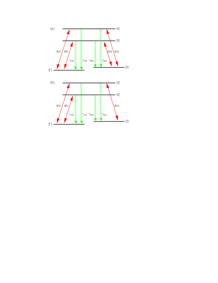
Figure 1: (Color online) The four-level double-$\Lambda$ type schemes considered in the analysis. (a) is driven by four laser fields indicated by the red arrows with Rabi frequencies $g_{ij}$ ($i\in\{3,4\}$,$j\in\{1,2\}$) that form a closed interaction loop. This loop gives rise to a dependence on the relative phase of the different laser fields, and in general makes a time-independent steady state of the system dynamics impossible. (b) is the corresponding level scheme where one of the driving fields has been removed ($g_{32}=0$). Here, the laser fields do not form a closed loop. The spontaneous decays with rates $\gamma_{ij}$ ($i\in\{1,2\}$,$j\in\{3,4\}$) are denoted by the wiggly green lines.

A peculiarity of the closed laser interaction loop systems is the fact that a certain initial atomic state is connected to another atomic state via several combinations of laser field interactions. On the one hand, this gives rise to a dependence of the optical properties of the system on the relative phase of the driving fields. This allows for a great control of the optical properties and has been exploited in various circumstances, as discussed above. The drawback, however, is that such a system in general does not have a time-independent steady state. A time-independent steady state is reached only if a particular linear combination of the detunings of all incident laser fields is zero, that is, if the so-called multiphoton resonance condition is fulfilled. This assumption was made in the previous studies. But for a meaningful definition of the group velocity of a probe pulse in a given medium, one has to require that the medium itself including the coupling fields, which in this context merely aid in the preparation of the medium, has properties independent of the probe pulse characteristics. While the probe pulse which is finite in time necessarily consists of different frequency components and thus interacts with the atom with different detunings, the coupling fields have to be kept fixed in the calculation of the probe field propagation, since the different frequency components interact with the medium simultaneously. In particular, it is not possible to adjust one of the coupling field detunings such that the multiphoton resonance condition is maintained throughout the pulse propagation. Thus, it is impossible to assume the multiphoton resonance condition in the evaluation of the propagation of a finite probe pulse, and a time-dependent analysis is required.

Therefore in this paper, we investigate the light propagation in a four-level double lambda system as shown in Fig. 1(a) both with and without assuming the multiphoton resonance condition. We apply laser fields to all four dipole-allowed transitions to generate a closed laser-interaction loop. In the time-independent case where the multiphoton resonance condition is fulfilled, we find sub- and superluminal light propagation, controlled simply by the relative phase of the driving fields. For the time-dependent study beyond the multiphoton resonance condition, we apply a Floquet decomposition to the in general time dependent equations of motion. By comparing the Floquet decomposition to the time-independent treatment, we identify the respective frequency components found in this expansion with different interaction pathways in the closed loop system. We find that the medium response oscillating in phase with the probe field in general is not phase-dependent. The phase-dependent process contributing to the probe field susceptibility only occurs at a specific frequency, and is thus likely to distort the shape of a short probe pulse considerably if this specific frequency is contained in the wide frequency spectrum of the short pulse. Thus we conclude that for parameters violating the multiphoton resonance condition as in the probe pulse propagation, inducing a closed loop interaction contour may not be advantageous. Nevertheless, we demonstrate that also under conditions without a closed loop as shown in Fig. 1(b), both sub- and superluminal light propagation is possible with gain. Finally, we identify the Rabi frequency of one of the coupling fields as a convenient control parameter which allows to switch between sub- and superluminal light propagation.

II Theoretical Analysis

II.1 The Model

We consider a four-level atomic systems in a double-$\Lambda$ configuration as depicted in Figure 1. The scheme consists of two metastable lower states $|1\rangle$, $|2\rangle$ and two excited states $|3\rangle$, $|4\rangle$. The electric-dipole allowed transitions $|1\rangle-|3\rangle$, $|2\rangle-|3\rangle$ and $|2\rangle-|4\rangle$ are driven by three coherent laser fields, while a weak tunable coherent probe field with central frequency $\omega_{p}=\omega_{41}$ is applied to the dipole-allowed transition $|1\rangle-|4\rangle$. The spontaneous decay rates from level $|i\rangle$ ($i\in\{3,4\}$) to the levels $|j\rangle$ ($j\in\{1,2\}$) are denoted by $2\gamma_{ji}$. The electromagnetic driving fields applied to transition $|i\rangle-|j\rangle$ can be written as

$$\bm{E}_{ij}=E_{ij}\hat{\bm{e}}_{ij}e^{-i(\omega_{ij}t-\vec{k}_{ij}\vec{r}+\phi_{ij})}+\textrm{ c.c.}\,,$$ (1)

with amplitude $E_{ij}$, unit polarization vectors $\hat{\bm{e}}_{ij}$, frequencies $\omega_{ij}$, wave vectors $\vec{k}_{ij}$ and absolute phase $\phi_{ij}$. Note that we do not assume absolute phase control in our calculations, but only relative phase control between the different driving fields.

The Hamiltonian in dipole and rotating wave approximation is given by scullybook ; FiSw2005

$$H= \sum_{j=1}^{4}E_{j}|j\rangle\langle j|$$

$$-\sum_{l=3}^{4}\sum_{m=1}^{2}\left(\hbar g_{lm}e^{-i\alpha_{lm}}|l\rangle\langle m|+\textrm{ h.c.}\right)\,,$$ (2)

where the corresponding Rabi frequencies are denoted by $g_{ij}=E_{ij}(\hat{\bm{e}}_{ij}\vec{d}_{ij})/\hbar$ with $\vec{d}_{ij}$ as the atomic dipole moment of the corresponding transition. The energies of the involved states are denoted $E_{i}$ ($i\in\{1,\dots,4\}$), and we define the transition frequencies $\bar{\omega}_{ij}=(E_{i}-E_{j})/\hbar$. The arguments of the exponential functions are given by

$$\alpha_{ij}=\omega_{ij}t-\vec{k}_{ij}\vec{r}+\phi_{ij}\,.$$ (3)

In a suitable reference frame, the Hamiltonian can be written as

$$V= \hbar(\Delta_{32}-\Delta_{31})\tilde{\rho}_{22}-\hbar\Delta_{31}\tilde{\rho}_{33}$$

$$+\hbar(\Delta_{32}-\Delta_{31}-\Delta_{42})\tilde{\rho}_{44}$$

$$-\hbar\left(g_{31}\tilde{\rho}_{31}+g_{32}\tilde{\rho}_{32}+g_{42}\tilde{\rho}_{42}\right.$$

$$\left.+g_{41}\tilde{\rho}_{41}e^{-i\Phi}+\textrm{ h.c.}\right)\,.$$ (4)

Here, we have defined $\rho_{ij}=|i\rangle\langle j|$ and the corresponding operator in the new reference frame is denoted by $\tilde{\rho}_{ij}$ ($i,j\in\{1,\dots,4\}$). It is interesting to note that now the residual time dependence along with the laser field phases appears only together with the probe field Rabi frequency $g_{41}$ in the parameter $\Phi$ given by

$$\Phi =\Delta t-\vec{K}\vec{r}+\phi_{0}\,,$$ (5a)

$$\Delta =(\Delta_{32}+\Delta_{41})-(\Delta_{31}+\Delta_{42})\,,$$ (5b)

$$\vec{K} =(\vec{k}_{32}+\vec{k}_{41})-(\vec{k}_{31}+\vec{k}_{42})\,,$$ (5c)

$$\phi_{0} =(\phi_{32}+\phi_{41})-(\phi_{31}+\phi_{42})\,.$$ (5d)

The parameters $\Delta$, $\vec{K}$ and $\phi_{0}$ are known as the multiphoton resonance detuning, wave vector mismatch and initial phase difference, respectively. Note that in general it is not possible to find a reference frame where the explicit time dependence due to $\Delta$ vanishes from the Hamiltonian, such that for $\Delta\neq 0$ no stationary long-time limit can be expected. Using the notations Eqs. (5) and Eq. (3), the transformation of the operator $\rho_{41}$, which will be of particular interest later on, to the chosen interaction picture can be written as

$$\tilde{\rho}_{41} =e^{-i\Phi}\,e^{i\alpha_{41}}\,\rho_{41}\,.$$ (6)

We further define $\hat{\rho}_{41}$ as the coherence $\rho_{41}$ in a reference frame oscillating in phase with the probe field $\bm{E}_{41}$ as

$$\hat{\rho}_{41} =e^{i\alpha_{41}}\,\rho_{41}=e^{i\Phi}\tilde{\rho}_{41}\,.$$ (7)

From the Hamiltonian Eq. (II.1), and including the spontaneous decay in Born-Markov approximation, the density matrix equations of motion can be derived as

$$\frac{\partial}{\partial t}\tilde{\rho}_{11} =ig^{\ast}_{31}\tilde{\rho}_{31}-ig_{31}\tilde{\rho}_{13}+ig^{\ast}_{41}\tilde{\rho}_{41}e^{i\Phi}$$

$$-ig_{41}\tilde{\rho}_{14}e^{-i\Phi}+2\gamma_{13}\tilde{\rho}_{33}+2\gamma_{14}\tilde{\rho}_{44}\,,$$ (8a)

$$\frac{\partial}{\partial t}\tilde{\rho}_{22} =ig^{\ast}_{32}\tilde{\rho}_{32}-ig_{32}\tilde{\rho}_{23}+ig^{\ast}_{42}\tilde{\rho}_{42}$$

$$-ig_{42}\tilde{\rho}_{24}+2\gamma_{23}\tilde{\rho}_{33}+2\gamma_{24}\tilde{\rho}_{44}\,,\allowdisplaybreaks[2]$$ (8b)

$$\frac{\partial}{\partial t}\tilde{\rho}_{33} =-ig^{\ast}_{31}\tilde{\rho}_{31}-ig^{\ast}_{32}\tilde{\rho}_{32}+ig_{31}\tilde{\rho}_{13}$$

$$+ig_{32}\tilde{\rho}_{23}-2\gamma_{3}\tilde{\rho}_{33}\,,\allowdisplaybreaks[2]$$ (8c)

$$\frac{\partial}{\partial t}\tilde{\rho}_{12} =i(\Delta_{32}-\Delta_{31})\tilde{\rho}_{12}+ig^{\ast}_{31}\tilde{\rho}_{32}-ig_{32}\tilde{\rho}_{13}$$

$$+ig^{\ast}_{41}\tilde{\rho}_{42}e^{i\Phi}-ig_{42}\tilde{\rho}_{14}-\Gamma_{12}\tilde{\rho}_{12}\,,\allowdisplaybreaks[2]$$ (8d)

$$\frac{\partial}{\partial t}\tilde{\rho}_{13} =-i\Delta_{31}\tilde{\rho}_{13}+ig^{\ast}_{31}(\tilde{\rho}_{33}-\tilde{\rho}_{11})-ig^{\ast}_{32}\tilde{\rho}_{12}$$

$$+ig^{\ast}_{41}\tilde{\rho}_{43}e^{i\Phi}-\Gamma_{13}\tilde{\rho}_{13}\,,\allowdisplaybreaks[2]$$ (8e)

$$\frac{\partial}{\partial t}\tilde{\rho}_{14} =i(\Delta_{32}-\Delta_{31}-\Delta_{42})\tilde{\rho}_{14}+ig^{\ast}_{41}e^{i\Phi}(\tilde{\rho}_{44}-\tilde{\rho}_{11})$$

$$-ig^{\ast}_{42}\tilde{\rho}_{12}+ig^{\ast}_{31}\tilde{\rho}_{34}-\Gamma_{14}\tilde{\rho}_{14}\,,\allowdisplaybreaks[2]$$ (8f)

$$\frac{\partial}{\partial t}\tilde{\rho}_{23} =-i\Delta_{32}\tilde{\rho}_{23}+ig^{\ast}_{32}(\tilde{\rho}_{33}-\tilde{\rho}_{22})-ig^{\ast}_{31}\tilde{\rho}_{21}$$

$$+ig^{\ast}_{42}\tilde{\rho}_{43}-\Gamma_{23}\tilde{\rho}_{23}\,,\allowdisplaybreaks[2]$$ (8g)

$$\frac{\partial}{\partial t}\tilde{\rho}_{24} =-i\Delta_{42}\tilde{\rho}_{24}+ig^{\ast}_{42}(\tilde{\rho}_{44}-\tilde{\rho}_{22})-ig^{\ast}_{41}\tilde{\rho}_{21}e^{i\Phi}$$

$$+ig^{\ast}_{32}\tilde{\rho}_{34}-\Gamma_{24}\tilde{\rho}_{24}\,,\allowdisplaybreaks[2]$$ (8h)

$$\frac{\partial}{\partial t}\tilde{\rho}_{34} =-i(\Delta_{42}-\Delta_{32})\tilde{\rho}_{34}+ig_{31}\tilde{\rho}_{14}+ig_{32}\tilde{\rho}_{24}$$

$$-ig^{\ast}_{41}\tilde{\rho}_{31}e^{i\Phi}-ig^{\ast}_{42}\tilde{\rho}_{32}-\Gamma_{34}\tilde{\rho}_{34}\,,\allowdisplaybreaks[2]$$ (8i)

$$\tilde{\rho}_{44} =1-\tilde{\rho}_{11}-\tilde{\rho}_{22}-\tilde{\rho}_{33}\,.$$ (8j)

We have further defined $\gamma_{j}=\gamma_{1j}+\gamma_{2j}$, and our chosen level scheme implies $\gamma_{1}=\gamma_{2}=0$. $\Gamma_{ij}=(2\gamma_{i}+2\gamma_{j})/2$ ($i\in\{1,2\}$ and $j\in\{3,4\}$) are the damping rates of the coherences on transitions $|i\rangle-|j\rangle$.

Due to the explicit time dependence of Eqs. (8) via the parameter $\Delta$ in $\Phi$, it is clear that in general the system does not have a constant steady state solution. If, however, the so-called multiphoton resonance condition $\Delta=0$, $\vec{K}=0$ is fulfilled, then the equations of motion (8) have constant coefficients and thus a stationary solution in the long-time limit can be found, which for a suitable choice of parameters depends on the constant relative phase $\phi_{0}$.

II.2 Linear susceptibility and group velocity

The linear susceptibility of the weak probe field can be written as scullybook ; FiSw2005

$$\chi(\omega_{p})=\frac{2Nd_{41}}{\epsilon_{0}E_{41}}\rho_{41}(\omega_{p})\,,$$ (9)

where $N$ is the atom number density in the medium and $\chi=\chi^{\prime}+i\chi^{\prime\prime}$. The real and imaginary parts of $\chi(\omega_{p})$ correspond to the dispersion and the absorption respectively. This expression for the susceptibility usually is applied to a single probe field frequency $\omega_{p}$ of a narrow-bandwidth continuous-wave laser field. If the probe field consists of short pulses such that the individual probe pulses have a non-negligible frequency width, then Eq. (9) describes the propagation of an individual frequency component of the probe pulse.

For a realistic example, we consider the sodium $D_{1}$ transition, in which the transition rate, dipole moment and atom density are $\gamma=2\pi\times 9.76$ MHz, $d_{41}=2.1\times 10^{-29}$ Cm and $N=1.3\times 10^{12}$ cm^-3, respectively. The probe field with $g_{41}=0.01\gamma$ is applied to the system, leading to $(2\,N\,d_{41})/(\epsilon_{0}E_{41})\simeq 1$. Eq. (9) refers to the part of the coherence $\rho_{41}(\omega_{p})$ oscillating at a frequency of the incident probe beam. This coincides with the transformed coherence $\hat{\rho}_{41}$ introduced in Eq. (7). Thus for our choice of example parameters, we obtain

$$\chi(\omega_{p})\simeq\hat{\rho}_{41}\,.$$ (10)

Therefore throughout our numerical study, we will discuss the transformed coherence $\hat{\rho}_{41}$ in order to be study the light propagation in the medium.

We also introduce the so-called group index, $n_{g}=c/v_{g}$ where $v_{g}$, the group velocity of the probe field, is given by scullybook ; FiSw2005

$$v_{g}=\frac{c}{1+2\pi\chi^{\prime}(\omega_{p})+2\pi\frac{\partial}{\partial\omega_{p}}\chi^{\prime}(\omega_{p})}$$ (11)

This expression shows that, for a small imaginary part $\chi^{\prime\prime}(\omega_{p})$ and positive steep dispersion, the group velocity is significantly reduced. On the other hand, strong negative dispersion can leads to an increase in the group velocity and even to a negative group velocity.

II.3 Multi-photon resonance approximation

In this section, we assume the multi-photon resonance condition $\Delta=0$, $\vec{K}=0$ to be fulfilled. Then, the coefficients of the density matrix equations Eqs. (8) do not have an explicit time dependence, and the system has a stationary steady state. In the particular case

$$\Delta_{31} =\Delta_{32}=\Delta_{41}=\Delta_{42}=0\,,$$ (12a)

$$\gamma =\gamma_{14}=\gamma_{24}=\gamma_{13}=\gamma_{23}\,,$$ (12b)

a simple analytical expression for the steady state solution of $\tilde{\rho}_{41}$ up to leading order in $g_{41}$ can be found:

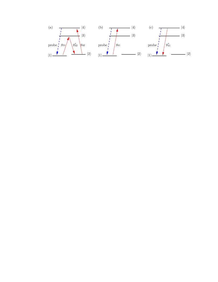
Figure 2: (Color online) Interpretation of the different contributions to the probe field susceptibility in terms of transition pathways. (a) represents the interaction loop leading to a scattering of the driving fields into the probe field mode. (b) is the direct scattering of the probe field off of the probe transition. (c) shows a counter-rotating term. The solid red arrows indicate coupling field transitions, the dashed blue line is a probe field interaction.

$$\tilde{\rho}_{41}= \frac{-i\,\gamma\,g_{32}^{\ast}\,g_{31}\,g_{42}}{2\,D}$$

$$+\frac{i\gamma^{3}\,(|g_{31}|^{2}+|g_{32}|^{2}+|g_{42}|^{2})\,|g_{32}|^{2}\,g_{41}e^{-i\phi_{0}}}{2\,D^{2}}$$

$$-\frac{i\gamma\,|g_{31}|^{2}\,|g_{32}|^{2}\,|g_{42}|^{2}\,g_{41}^{\ast}e^{i\phi_{0}}}{2\,D^{2}}\,,$$ (13)

where

$$D= |g_{31}|^{2}\cdot|g_{42}|^{2}+\gamma^{2}\left(|g_{31}|^{2}+|g_{32}|^{2}+|g_{42}|^{2}\right)\,.$$ (14)

Transferring to the frame rotating in phase with the probe field using Eqs. (6) and (7), we obtain

$$\hat{\rho}_{41}= \frac{-i\,\gamma\,g_{32}^{\ast}\,g_{31}\,g_{42}\,e^{i\phi_{0}}}{2\,D}$$

$$+\frac{i\gamma^{3}\,(|g_{31}|^{2}+|g_{32}|^{2}+|g_{42}|^{2})\,|g_{32}|^{2}\,g_{41}}{2\,D^{2}}$$

$$-\frac{i\gamma\,|g_{31}|^{2}\,|g_{32}|^{2}\,|g_{42}|^{2}\,g_{41}^{\ast}e^{2i\phi_{0}}}{2\,D^{2}}\,.$$ (15)

First, we note that the whole expression for $\hat{\rho}_{41}$ oscillates with same frequency as the probe field, as evidenced by the lack of an overall time-dependent factor in $\hat{\rho}_{41}$, and therefore contributes to the probe field susceptibility. The three contributions to Eq. (II.3) admit a simple interpretation in terms of the involved physical processes. The first component is proportional to $g_{32}^{\ast}\,g_{31}\,g_{42}$, and thus corresponds to a closed interaction loop involving a sequence of all four dipole-allowed transitions, or a scattering of the driving field modes into the probe field mode. This round-trip depends on the relative multiphoton phase $\phi_{0}$, which therefore occurs in this contribution. The second term in Eq. (II.3) proportional to $g_{14}$ represents a direct scattering of the probe field off of the probe transition, involving an excitation and a de-excitation of the probe transition. Since no closed interaction-contour via different laser fields is involved, this contribution does not depend on the relative phase $\phi_{0}$. The last contribution in Eq. (II.3) proportional to $g_{14}^{\ast}$ depends on twice the relative field phase $\phi_{0}$ can be interpreted as a counter-rotating contribution. This preliminary interpretation of the individual contributions will become more transparent in the time-dependent analysis without the assumption of multiphoton resonance in the following Sec. II.4.

II.4 Beyond the multi-photon resonance approximation

We now drop the multi-photon resonance condition and evaluate the equations of motion Eqs. (8) for the general case of time-dependent coefficients. The Eqs. (8) can be written in a compact form

$$\frac{\partial}{\partial t}\tilde{R}+\Sigma=M\tilde{R},$$ (16)

where

$$\tilde{R}= (\tilde{\rho}_{11},\tilde{\rho}_{12},\tilde{\rho}_{13},\tilde{\rho}_{14},\tilde{\rho}_{21},\tilde{\rho}_{22},\tilde{\rho}_{23},\tilde{\rho}_{24},$$

$$\tilde{\rho}_{31},\tilde{\rho}_{32},\tilde{\rho}_{33},\tilde{\rho}_{34},\tilde{\rho}_{41},\tilde{\rho}_{42},\tilde{\rho}_{43})^{T}$$ (17)

is a vector containing the density matrix elements, and

$$\Sigma= (-2\gamma_{14},0,0,-i\bar{g}^{\ast}_{41}e^{i\Delta t},0,-2\gamma_{24},$$

$$0,-ig^{\ast}_{42},0,0,0,0,i\bar{g}_{41}e^{-i\Delta t},ig_{42},0)^{T}$$ (18)

is a vector independent of the density matrix elements which arises from eliminating one of the state populations from the equations of motion via the trace condition $Tr(\tilde{\rho})=1$. Note that we have introduced the notation

$$\bar{g}_{41}=g_{41}\,e^{-i\vec{K}\vec{r}+i\phi_{0}}\,.$$ (19)

The matrix $M$ follows from Eqs. (8). Both the matrix $M$ and the $\Sigma$ can be separated into terms with different time dependence Hu ,

$$\Sigma =\Sigma_{0}+\bar{g}_{41}\Sigma_{1}e^{-i\Delta t}+\bar{g}^{\ast}_{41}\Sigma_{-1}e^{i\Delta t}\,,$$ (20a)

$$M =M_{0}+\bar{g}_{41}M_{1}e^{-i\Delta t}+\bar{g}^{\ast}_{41}M_{-1}e^{i\Delta t}\,,$$ (20b)

where $\Sigma_{0},\Sigma_{\pm 1},M_{0}$ and $M_{\pm 1}$ are time independent. Using these definitions in Eq. (16), we obtain

$$\frac{\partial}{\partial t}\tilde{R}+\Sigma_{0}+\bar{g}_{41}e^{-i\Delta t}\Sigma_{+1}+\bar{g}^{\ast}_{41}e^{i\Delta t}\Sigma_{-1}$$

$$=(M_{0}+\bar{g}_{41}e^{-i\Delta t}M_{1}+\bar{g}^{\ast}_{41}e^{i\Delta t}M_{-1})\tilde{R}\,.$$ (21)

It is important to note that the time dependence of Eqs. (8) only arises from the parameter $\Delta$, such that the coefficients are periodic in time. According to Floquet’s theorem floquet , the solution $\tilde{R}$ therefore has only contributions oscillating at harmonics of the detuning $\Delta$. The higher-order harmonics in this frequency expansion are suppressed by powers of the probe field Rabi frequency $g_{41}$ relative to the other frequencies involved in the system. Since we are interested in the case where the probe field is weak, we truncate the Floquet expansion after the leading first order and obtain as ansatz for the solution $\tilde{R}$:

$$\tilde{R}=\tilde{R}_{0}+\bar{g}_{41}e^{-i\Delta t}\tilde{R}_{1}+\bar{g}_{41}^{\ast}e^{i\Delta t}\tilde{R}_{-1}\,.$$ (22)

By using Eq. (22) in Eq. (II.4) and equating the coefficients oscillating at different harmonics of $\Delta$, we obtain the solutions for $\tilde{R}_{0}$ and $\tilde{R}_{\pm 1}$ as

$$\tilde{R}_{0} = M^{-1}_{0}\Sigma_{0}\,,$$ (23a)

$$\tilde{R}_{1} = (M_{0}+i\Delta)^{-1}(\Sigma_{1}-M_{1}\tilde{R}_{0})\,,$$ (23b)

$$\tilde{R}_{-1} = (M_{0}-i\Delta)^{-1}(\Sigma_{-1}-M_{-1}\tilde{R}_{0})\,.$$ (23c)

The medium response is determined by the 13th component $\tilde{\rho}_{41}$ of $\tilde{R}$. Transferring back $\tilde{\rho}_{41}$ to the operator $\hat{\rho}_{41}$ in the frame oscillating in phase with the probe field using Eqs. (6) and (7), we obtain

$$\hat{\rho}_{41}=[\tilde{R}_{0}]_{13}\,e^{i\Phi} +g_{41}[\tilde{R}_{1}]_{13}+g_{41}^{\ast}[\tilde{R}_{-1}]_{13}\,e^{2i\Phi}\,.$$ (24)

Here, $[x]_{13}$ denotes the 13th component of $x$. It can be seen that the contribution proportional to $[\tilde{R}_{1}]_{13}$ oscillates in phase with the probe beam, and thus contributes to the probe beam susceptibility independent of the frequency of the incident driving field. For $\Delta\neq 0$, the two other contributions proportional to $[\tilde{R}_{0}]_{13}$ and $[\tilde{R}_{-1}]_{13}$ oscillate at different frequencies due to the time dependence of $\Phi$ and thus do not contribute to the probe beam susceptibility. However, even in the case $\Delta\to 0$, the term $[\tilde{R}_{1}]_{13}$ is distinct in that the two other contributions in general propagate differently due to the wave vector mismatch $\vec{K}$.

Using the result Eq. (24), we are now also in the position to in detail understand the expression Eq. (II.3) we previously derived assuming $\Delta=0$ and $\vec{K}=0$. For this, we explicitly evaluate $[\tilde{R}_{0}]_{13}$, $[\tilde{R}_{1}]_{13}$ and $[\tilde{R}_{-1}]_{13}$ using the parameters Eq. (12) as well as $\Delta=0$ and obtain

$$[\tilde{R}_{0}]_{13}\,e^{i\Phi} =\frac{-i\gamma g_{32}^{\ast}\,g_{31}\,g_{42}}{2D}e^{-\vec{K}\vec{r}+\phi_{0}}\,,$$ (25a)

$$g_{41}\,[\tilde{R}_{1}]_{13} =\frac{i\gamma^{3}\,(|g_{31}|^{2}+|g_{32}|^{2}+|g_{42}|^{2})\,|g_{32}|^{2}\,g_{41}}{2D^{2}}\,,$$ (25b)

$$g_{41}^{\ast}\,[\tilde{R}_{-1}]_{13}\,e^{2i\Phi} =\frac{-i\gamma\,(|g_{31}|^{2}\,|g_{32}|^{2}\,|g_{42}|^{2})\,g_{41}^{\ast}}{2D^{2}}e^{-2\vec{K}\vec{r}+2\phi_{0}}\,.$$ (25c)

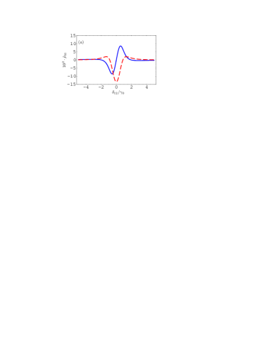
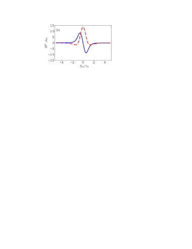
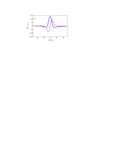
Figure 3: (Color online) Real (blue solid line) and imaginary (red dashed line) parts of the atomic density matrix element $\hat{\rho}_{41}$ in a reference frame oscillating in phase with the probe field as a function of the Raman detuning $\delta_{12}=\Delta_{31}-\Delta_{32}=\Delta_{41}-\Delta_{42}$. The real part corresponds to the probe field dispersion, whereas the imaginary part describes the absorptive properties. The relative initial phase difference between the four applied laser fields is $\phi_{0}=0$ in (a), $\phi_{0}=\pi$ in (b) and $\phi_{0}=\pi/2$ in (c). The common parameters are $2\gamma_{13}=2\gamma_{14}=2\gamma_{23}=2\gamma_{24}=\gamma_{0}$, and thus $\Gamma_{13}=\Gamma_{14}=\Gamma_{23}=\Gamma_{24}=\gamma_{0}$, $\Gamma_{12}=0.0$, and $\Gamma_{34}=2\gamma_{0}$. The detunings are $\Delta_{32}=\Delta_{42}=0$, and the Rabi frequencies are chosen as $g_{31}=g_{32}=g_{42}=0.6\gamma_{0}$ and $g_{41}=0.01\gamma_{0}$.

Note that $D$ is defined in Eq. (14). Thus the time-dependent Floquet decomposition in the limit $\Delta\to 0$, $\vec{K}\to 0$ yields exactly the result Eq. (II.3) of the time-independent analysis, as expected. The first part of Eq. (II.3) representing the scattering of the driving fields into the probe field mode arises from $[\tilde{R}_{0}]_{13}$, as shown in Fig. 2(a). This contribution in general does not oscillate at the probe field frequency, but rather at the combination frequency $\omega_{31}+\omega_{42}-\omega_{32}$ of the three driving fields. This frequency coincides with the probe field frequency only under multiphoton resonance. The contribution proportional to $[\tilde{R}_{1}]_{13}$ shown in Fig. 2(b) is in phase with the probe field for all values of $\Delta$, and is independent of the relative field phase. It represents the direct scattering of the probe field off of the probe field transition. The third contribution proportional to $[\tilde{R}_{-1}]_{13}$ can be interpreted as a counter-rotating term which in the Floquet expansion differs by $2\Delta$ from the probe field frequency, and is depicted in Fig. 2(c).

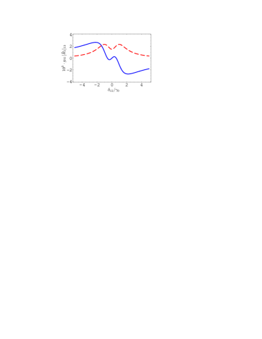
Figure 4: (Color online) Real (blue solid line) and imaginary (red dashed line) parts of the contribution to the Floquet decomposition representing the direct scattering of the probe field off of the probe transition, $g_{41}\,[\tilde{R}_{1}]_{13}$ [see Eq. (24)]. This figure depicts one of the processes contributing to the results in Fig. 3, and the parameters are the same as in this figure. Note that this particular contribution is independent of the phase $\phi_{0}$, such that only one subfigure is shown, consistent with the interpretation in Sec. II.4.

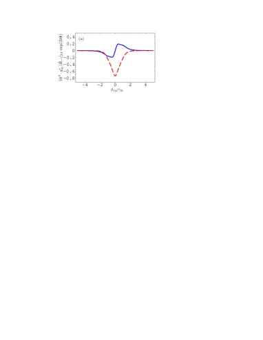
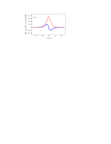
Figure 5: (Color online) Real (blue solid line) and imaginary (red dashed line) parts of the contribution to the Floquet decomposition representing a counter-rotating contribution, $g_{41}^{\ast}\,[\tilde{R}_{-1}]_{13}\,\exp(2i\Phi)$ [see Eq. (24)]. This figure depicts one of the processes contributing to the results in Fig. 3, and the parameters are the same as in this figure. This particular contribution depends on the phase $2\phi_{0}$, such subfigure (a) shows the result for $\phi_{0}=0,\pi$ and (b) for $\phi=\pi/2$, consistent with the interpretation in Sec. II.4.

As an important result, we thus conclude that the phase-dependence of the loop-configuration studied here is restricted to the multiphoton resonance condition $\Delta=0$, because it arises from the scattering of the coupling fields into the probe field mode. Furthermore, it can be seen that all contributions but the direct scattering acquire an additional dependence on the wave vector mismatch $\vec{K}$, which influences the spatial emission pattern of these contributions. In general, only the direct scattering contribution can be detected in propagation direction of the probe beam regardless of the separation of detector and the scattering atoms. Finally, we note that the first expression $[\tilde{R}_{0}]_{13}$ is independent of $\Delta$, whereas $[\tilde{R}_{1}]_{13}$ and $[\tilde{R}_{-1}]_{13}$ have complicated dependencies on $\Delta$.

III Results and discussion

We now turn to the numerical study of our results from the master equations (8). In a first step we assume that the multiphoton resonance condition $\Delta=0,\vec{K}=0$ is fulfilled. Then the steady state solution for Eqs. (8) exist and depends on the initial constant relative phase $\phi_{0}$ of the driving fields [see, e.g., Eq. (II.3) for the special case of parameters Eq. (12)]. In Fig. 3 we plot the absorption and dispersion spectrum versus the Raman detuning $\delta_{12}=\Delta_{31}-\Delta_{32}=\Delta_{41}-\Delta_{42}$, for different initial phases $\phi_{0}$. The common parameters are chosen as $2\gamma_{13}=2\gamma_{14}=2\gamma_{23}=2\gamma_{24}=\gamma_{0}$, where $\gamma_{0}$ is the total decay rate of one of the upper transitions to a lower transition. Then, $\Gamma_{13}=\Gamma_{14}=\Gamma_{23}=\Gamma_{24}=\gamma_{0}$, $\Gamma_{12}=0$, and $\Gamma_{34}=2\gamma_{0}$. Further, $\Delta_{32}=\Delta_{42}=0$, and the driving fields have Rabi frequencies $g_{13}=g_{23}=g_{24}=0.6\gamma_{0}$, $g_{14}=0.01\gamma_{0}$. The initial phase values in Fig. 3 are $\phi_{0}=0$ in (a), $\phi_{0}=\pi$ in (b) and $\phi_{0}=\pi/2$ in (c). The slope of the dispersion (real part) is positive for $\phi_{0}=0$, and accompanied by gain (negative imaginary part). For $\phi_{0}=\pi$, however, the slope of the dispersion becomes negative together with an absorption peak. For $\phi_{0}=\pi/2$, the curve shapes of real and imaginary part are interchanged. The results show the phase-dependence of the probe absorption for a closed-loop configuration in good agreement with previous results as in Ref. Korsunsky .

We now evaluate the individual contributions to the Floquet decomposition of the density matrix, Eqs. (24), using the same parameters as above in Fig. (3). From Eq. (24), it is obvious that the numerically dominant contribution arises from $[\tilde{R}_{0}]_{13}\,\exp(i\Phi)$, since the two other contributions are suppressed by one power of the weak driving field Rabi frequency $g_{41}$. Consistent with this interpretation, the results for $[\tilde{R}_{0}]_{13}\,\exp(i\Phi)$ are almost identical to the ones shown in Fig. 3, with the difference given by the two other terms in Eq. (24) and the neglected higher-order terms of order $\mathcal{O}(g_{41}^{2})$. Therefore, in the following, we only show the two difference contributions $g_{41}[\tilde{R}_{1}]_{13}$ and $g_{41}^{\ast}[\tilde{R}_{-1}]_{13}\,\exp(2i\Phi)$. Fig. 4 shows the contribution $g_{41}[\tilde{R}_{1}]_{13}$, which is the process contributing to the results in Fig. 3 depicted in Fig. 2(b). As discussed in Sec. II.4, this process is insensitive to the phase $\phi_{0}$, such that only one subfigure is shown for all values of $\phi_{0}$. Note that the results confirm our expectation that the numerical contribution of this process to the full results in Fig. 3 is small. The contribution $g_{41}^{\ast}[\tilde{R}_{-1}]_{13}\,\exp(2i\Phi)$ is shown in Fig. 5; the corresponding process is depicted in Fig. 2(c). This process depends on $2\phi_{0}$, such that subfigure (a) shows the identical results for $\phi_{0}=0$ and $\phi_{0}=\pi$, whereas subfigure (b) shows the result for $\phi_{0}=\pi/2$. Also the numerical contribution of this process to Fig. 3 is small as compared to $[\tilde{R}_{0}]_{13}\,\exp(i\Phi)$.

As discussed in Secs. I and II.2, the slope of the dispersion spectrum against the probe field detuning has a major role in the calculation of the group velocity. But to define the group velocity of a probe pulse in a given medium properly, one has to require that the medium itself including the coupling fields has properties independent of the probe pulse characteristics. Note that in this context the coupling fields prepare the medium, and in that sense belong to the medium in which the probe pulse propagates, and thus their detunings needs to be kept fixed. The probe pulse, however, has a finite duration and thus consists of different frequency components which interact with the atom with different detunings simultaneously. In particular, it is not possible to, e.g., adjust one of the coupling field detunings such that the multiphoton resonance condition is maintained throughout the pulse propagation. Therefore, the propagation of a pulse cannot be described assuming the multiphoton resonance condition, and our numerical results Fig. 3-5 presented so far are not sufficient to evaluate the group velocity.

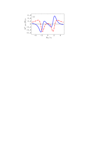
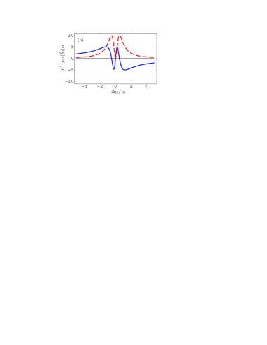
Figure 6: (Color online) Real (blue solid line) and imaginary (red dashed line) parts of the contribution to the Floquet decomposition representing the direct scattering of the probe field off of the probe transition, $g_{41}\,[\tilde{R}_{1}]_{13}$ [see Eq. (24)]. The susceptibility is plotted against the probe field detuning $\Delta_{41}$. This corresponds to a calculation relevant for the evaluation of the group velocity, but violates the multiphoton resonance condition and thus requires a Floquet analysis. The parameters in (a) are $\Delta_{31}=\Delta_{32}=\Delta_{42}=0$, $2\gamma_{13}=2\gamma_{14}=2\gamma_{23}=2\gamma_{24}=\gamma_{0}$, $g_{31}=1.8\gamma_{0}$, $g_{32}=0.2\gamma_{0}$, $g_{42}=0.5\gamma_{0}$, and $g_{41}=0.01\gamma_{0}$. Subfigure (b) shows the case $\Delta_{31}=10\gamma_{0}$, $\Delta_{32}=\Delta_{42}=0$, $2\gamma_{13}=2\gamma_{14}=2\gamma_{23}=2\gamma_{24}=\gamma_{0}$, $g_{31}=g_{32}=0.1\gamma_{0}$, $g_{42}=0.5\gamma_{0}$, and $g_{41}=0.01\gamma_{0}$.

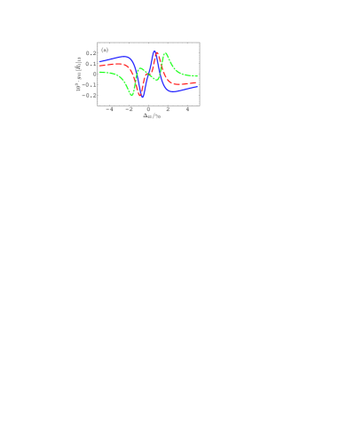
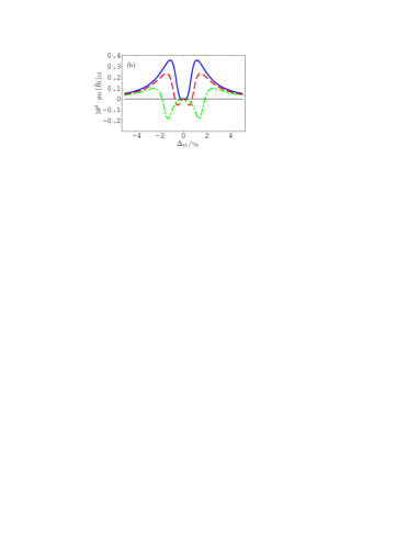
Figure 7: (Color online) Real (a) and imaginary (b) parts of the scaled contribution to the Floquet decomposition representing the direct scattering of the probe field off of the probe transition, $[\tilde{R}_{1}]_{13}$ [see Eq. (24)]. The susceptibility is plotted against the probe field detuning $\Delta_{41}$ with other detunings chosen as $\Delta_{31}=\Delta_{42}=0$. One of the Rabi frequencies is chosen as zero, $g_{32}=0$, such that the setup corresponds to the one shown in Fig 1(b). The solid blue line is for $g_{31}=0.7\gamma_{0}$, the red dashed line for $g_{31}=0.85\gamma_{0}$, and the green dash-dotted line for $g_{31}=1.5\gamma_{0}$. The other parameters are $2\gamma_{13}=2\gamma_{14}=2\gamma_{23}=2\gamma_{24}=\gamma_{0}$, $g_{42}=0.2\gamma_{0}$, and $g_{41}=0.01\gamma_{0}$.

Therefore, in Fig. 6(a), we show the probe field susceptibility against the probe field detuning $\Delta_{41}$, while the coupling field detunings are $\Delta_{31}=\Delta_{32}=\Delta_{42}=0$. This corresponds to a calculation relevant for the evaluation of the group velocity, but violates the multiphoton resonance condition $\Delta=0$ for most values of $\Delta_{41}$ shown in the figure and thus requires the use of the time-dependent Floquet analysis. Consequently, in Fig. 6, we only show the component $[\tilde{R}_{1}]_{13}$ since this part of the Floquet decomposition is the only one which oscillates in phase with the probe field under these conditions. It can be seen in Fig. 6(a) that around $\Delta_{41}=\pm 2\,\gamma_{0}$, the real part of the susceptibility has positive slope, while the imaginary part is strongly negative. This indicates subluminal light propagation with gain. At about $\Delta_{41}=0$, the real part of the susceptibility has negative slope over a wide frequency range, together with a small positive or even negative imaginary part. This corresponds to superluminal propagation with small absorption or gain.

If, however, the parameters and the laser field alignments are such that for a particular value of $\Delta_{41}$ within the resonance structure in the susceptibility the multiphoton resonance condition is fulfilled, then the coupling fields may be scattered into the probe field mode. This would give rise to a huge, very narrow contribution to the probe field susceptibility [see Fig. 3], which is likely to completely distort the probe pulse shape. In Fig. 6(a), this could occur at $\Delta_{41}=0$ if the laser field wavevectors are chosen suitably. Therefore for probe pulse propagation, parameters may be favorable which suppress the scattering of the coupling fields into the probe field mode. But under such conditions, the system is not phase-dependent.

In Fig. 6(b), we show a case where the multiphoton resonance condition $\Delta=0$ is violated for all shown values of $\Delta_{41}$. This avoids the scattering of the coupling fields into the probe field mode, and is accomplished by choosing the detunings as $\Delta_{31}=10\,\gamma_{0}$, and $\Delta_{32}=\Delta_{42}=0$. Around $\Delta_{41}=0$, subluminal light propagation with little absorption can be achieved. The fact that this and similar result can be obtained for a rather large detuning $\Delta_{31}=100\,g_{31}$ as compared to the corresponding Rabi frequency then suggest that a closed-loop configuration of the laser fields may not be necessary at all.

Therefore, in the final part, we discuss the dispersion and absorption spectrum for the system without a closed interaction loop shown in Fig. 1(b). Fig. 7 shows again the probe field susceptibility due to the direct scattering of the probe beam off of the probe transitions, with Rabi frequency $g_{32}=0$. Subfigure (a) shows the real part, (b) the imaginary part. The solid blue line is for $g_{31}=0.7\gamma_{0}$, the red dashed line for $g_{31}=0.85\gamma_{0}$, and the green dash-dotted for $g_{31}=1.5\gamma_{0}$. All coupling field detunings are zero, and the other parameters are $2\gamma_{13}=2\gamma_{14}=2\gamma_{23}=2\gamma_{24}=\gamma_{0}$, $g_{42}=0.2\gamma_{0}$, and $g_{41}=0.01\gamma_{0}$. If the Rabi frequency $g_{31}$ for transition $|1\rangle-|3\rangle$ is small, then the results are similar to the simple three-level electromagnetically induced transparency (EIT) case. The slope of the dispersion is positive, and subluminal light propagation appears with an EIT dip in the absorption spectrum, see the solid blue line in Fig. 7. With increasing Rabi frequency, the slope of the dispersion around zero detuning becomes negative and superluminal light propagation sets in. Together with superluminal light propagation, zero absorption or even gain is achieved. Thus the intensity of the pump fields can be used as a simple control parameter to switch the light propagation from subluminal to superluminal.

Fig. 8 shows another set of results for the system in Fig. 1(b), with parameters $\Delta_{42}=-5\gamma_{0}$, $\Delta_{31}=0$, $g_{32}=0$, $2\gamma_{13}=2\gamma_{14}=2\gamma_{23}=2\gamma_{24}=\gamma_{0}$, $g_{42}=0.6\gamma_{0}$, and $g_{41}=0.01\gamma_{0}$, and $g_{31}=0.7\gamma_{0}$ for the solid blue line, $g_{31}=0.85\gamma_{0}$ for the red dashed line, and $g_{31}=0.85\gamma_{0}$ for the green dash-dotted line. Due to the different coupling field detuning $\Delta_{42}$, the interesting probe susceptibility structure is shifted to $\Delta_{41}\approx-5\gamma_{0}$. In this region, for $g_{13}=0.8\gamma$, one finds subluminal light propagation accompanied by strong gain. Increasing the Rabi frequency $g_{13}$, again the light propagation switches to superluminal, still together with gain.

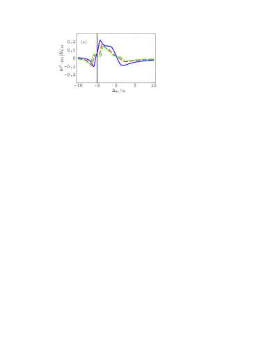
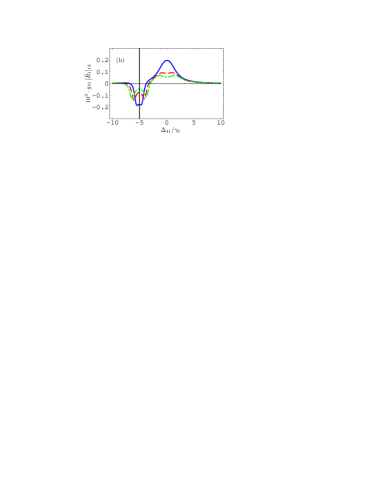
Figure 8: (Color online) As in Fig. 7, but with parameters $g_{31}=0.7\gamma_{0}$ for the solid blue line, $g_{31}=0.85\gamma_{0}$ for the red dashed line, and $g_{31}=0.85\gamma_{0}$ for the green dash-dotted line. The other parameters are $\Delta_{42}=-5\gamma_{0}$, $\Delta_{31}=0$, $g_{32}=0$, $2\gamma_{13}=2\gamma_{14}=2\gamma_{23}=2\gamma_{24}=\gamma_{0}$, $g_{42}=0.6\gamma_{0}$, and $g_{41}=0.01\gamma_{0}$. The solid vertical line indicates $\Delta_{41}=4\gamma_{0}$.

IV Discussion and summary

We have discussed the propagation of a probe pulse through a medium that is driven by coupling and probe laser fields that form a closed interaction loop. This gives rise to a dependence of the system on the relative phase of the various laser fields, but in general prohibits the existence of a time-independent steady state of the system. A stationary steady state only exists if the so-called multiphoton resonance condition $\Delta=0$ [see Eq. (5)] is fulfilled. A probe pulse, however, has a finite frequency width. Therefore, a time-independent analysis is insufficient to correctly describe the pulse propagation through the medium. To solve this problem, we have solved the time-dependent system without assuming the multiphoton resonance condition by means of a Floquet decomposition of the equations of motion. We found that the different Floquet components can be interpreted in terms of different scattering processes. The phase dependence arises from a scattering of the coupling fields into the probe field mode, and thus only occurs at a specific probe field frequency. If this frequency is within the frequency width of the probe pulse, a strong distortion of the pulse shape can be expected. In some cases, it may be possible to find probe pulses that are sufficiently narrow in the frequency domain such that they fit into the frequency range where the scattering of the coupling fields into the probe field mode dominates. Especially for shorter and thus broader pulses, however, we conclude that it may be advantageous to avoid the scattering of the coupling fields into the probe field mode. Then, however, the system is no longer phase dependent, and a closed interaction loop may not be necessary at all. We expect that similar results hold for other level schemes which involve a closed laser field interaction loop.

Apart from these general considerations, using our time-dependent Floquet analysis, we have shown that for realistic parameter sets both the closed-loop double-$\Lambda$ system and the corresponding system without a closed loop allow for sub- and superluminal light propagation with small absorption or even with gain. Further, we have identified the Rabi frequency of one of the coupling fields as a convenient control parameter to switch the light propagation between sub- and superluminal light propagation.

- (1) S. E. Harris, J. E. Field, and A. Kasapi, Phys. Rev. A 46, R29 (1992); A. Kasapi, M. Jain, G. Y. Yin, and S. E. Harris, Phys. Rev. Lett. 74,2447 (1995).
- (2) O. Schmidt, R. Wynands, Z. Hussein, and D. Meschede, Phys. Rev. A, 53, R27 (1996); G. Muller, A. Wicht, R. Rinkleff, and K. Danzmann, Opt. Commun. 127,37 (1996).
- (3) J. E. Field, K. H. Hahn, and S. E. Harris, Phys. Rev. Lett. 67,3062 (1991); S. E. Harris, J. E. Field, and A. Imamoglu, Phys. Rev. Lett. 64,1107 (1990); S. E. Harris, Phys. Today, 50, (7),36 (1997).
- (4) M. Xiao, Y. Q. Li , S. Z. Jin , and J. Gea-Banacloche, Phys. Rev. Lett. 74, 666(1995); D. Budker, D. F. Kimball, S. M. Rochester, and V. V. Yashchuk, Phys. Rev. Lett. 83, 1767 (1999).
- (5) L. V. Hau, S. E. Harris, Z. Dutton and C. H. Behroozi, Nature (London) 394, 594 (1999).
- (6) M. M. Kash, V. A. Sautenkov, A. S. Zibrov, L. Hollberg, G. R. Welch, M. D. Lukin, Y. Rostovtsev, E. S. Fry, and M. O. Scully, Phys. Rev. Lett. 82, 5229(1999); S. B. Ham, P. R. Hemmer, and M. S. Shahriar, Opt. Commun. 144, 227 (1997).
- (7) A. M. Steinberg and R. Y. Chiao, Phys. Rev A 49, 2071 (1994); E. L. Bolda, J. C. Garrison, R. Y. Chiao, Phys. Rev. A 49, 2938 (1994).
- (8) L. J. Wang, A. Kuzmich and A. Dogariu, Nature (London) 406, 277 (2000); A. Dogariu, A. Kuzmich and L. J. Wang, Phys. Rev. A 63, 053806 (2001); A. Kuzmich, A. Dogariu, L. J. Wang, P. W. Milonni and R. Y. Chiao, Phys. Rev. Lett. 86, 3925 (2001); A. Dogariu, A. Kuzmich, H. Cao, and L. J. Wang, Opt. Express. 8, 344 (2003).
- (9) R. Y. Chiao and A. M. Steinberg, in: Progress in Optics XXXVII, ed. E. Wolf (Elsevier, Amsterdam, 1997), p.345.
- (10) K. Kim, H. S. Moon, C. Lee, S. K. Kim, and J. B. Kim, Phys. Rev. A 68, 013810 (2003).
- (11) Md. A. I. Talukder, Y. Amagishi and M. Tomita, Phys. Rev. Lett. 86, 3546 (2001).
- (12) Y. Shimizu, N. Shiokawa, N. Yamamoto, M. Kozuma, T. Kuga, L. Deng, and E. W. Hagley, Phys. Rev. Lett. 89, 233001 (2002).
- (13) C. Goren, A. D. Wilson-Gordon, M. Rosenbluh, and H. Friedmann, Phys. Rev. A 68, 043818 (2003).
- (14) G. S. Agarwal, T. N. Dey and S. Menon, Phys. Rev. A 64, 053809 (2001).
- (15) D. Han, H. Guo, Y. Bai, and H. Sun, Phys. Lett. A 334, 243 (2005).
- (16) H. Tajalli and M. Sahrai, J. Opt. B: Quant. Semiclass. Opt. 7, 168 (2005).
- (17) D. Bortman-Arbiv, A. D. Wilson-Gordon, and H. Friedmann, Phys. Rev. A 63, 043818 (2001).
- (18) M. Sahrai, H. Tajalli, K.T. Kapale, and M. S. Zubairy, Phys. Rev. A 70, 023813 (2004).
- (19) M. Mahmoudi, M. Sahrai and H. Tajalli, J. Phys. B: At. Mol. Opt. Phys. 39, 1825 (2006).
- (20) M. Mahmoudi, M. Sahrai and H. Tajalli, Phys. Lett. A 357, 66 (2006).
- (21) M. Sahrai, M. Mahmoudi and H. Tajalli, Submitted.
- (22) E. A. Korsunsky, N. Leinfellner, A. Huss, S. Baluschev, and L. Windholz, Phys. Rev. A 59, 2302 (1999); A. F. Huss, E. A. Korsunsky, and L. Windholz, J. Mod. Opt. 49 , 141 (2002).
- (23) O. Kocharovskaya and P. Mandel, Phys. Rev. A 42, 523 (1990); C. H. Keitel, O. A. Kocharovskaya, L. M. Narducci, M. O. Scully, S.-Y. Zhu, and H. M. Doss, Phys. Rev. A 48, 3196 (1993).
- (24) D. Kosachiov, B. G. Matisev and Y. V. Rozhdestvensky, Europhys. Lett. 22, 11 (1993).
- (25) E. Cerboneschi and E. Arimondo, Phys. Rev. A 52, R1823 (1995).
- (26) M. D. Lukin, P. R. Hemmer, M. Löffler and M. O. Scully, Phys. Rev. Lett. 81, 2675 (1998).
- (27) Y. F. Li, J. F. Sun, X. Y. Zhang, and Y. C. Wang, Opt. Commun. 202, 97 (2002).
- (28) W. Maichen, F. Renzoni, I. Mazets, E. Korsunsky and L. Windholz, Phys. Rev. A 53, 3444 (1996).
- (29) G. Morigi, S. Franke-Arnold, and G.-L. Oppo, Phys. Rev. A 66, 053409 (2002).
- (30) E. A. Korsunsky and D. V. Kosachiov, Phys. Rev. A 60, 4996 (1999).
- (31) Z. Ficek and S. Swain, Quantum Interference and Coherence: Theory and Experiments (Springer, Berlin, 2005).
- (32) M. O. Scully and M. S. Zubairy, Quantum Optics (Cambridge University Press, Cambridge, 1997).
- (33) G. Floquet, Ann. École Norm. Sup. 12, 47 (1883); V. I. Ritus, Zh. Éksp. Teor. Fiz. 51, 1544 (1966); Y. B. Zeldovich, Zh. Éksp. Teor. Fiz. 51, 1006 (1966).
- (34) X.-m. Hu, D. Du, G.-l. Cheng, J.-h. Zou and X. Li, J. Phys. B: At. Mol. Opt. Phys. 38, 827(2005).