Keeping a Quantum Bit Alive by Optimized -Pulse Sequences
Abstract
A general strategy to maintain the coherence of a quantum bit is proposed. The analytical result is derived rigorously including all memory and back-action effects. It is based on an optimized -pulse sequence for dynamic decoupling extending the Carr-Purcell-Meiboom-Gill (CPMG) cycle. The optimized sequence is very efficient, in particular for strong couplings to the environment.
pacs:
03.67.Pp,03.67.Lx,03.65.Yz,03.65.VfQuantum information processing is a very promising and very challenging concept Zoller et al. (2005). The basic feature which makes quantum information conceptually more powerful than classical information is the quantum mechanical superposition principle. It allows for the parallel processing of many classical registers – the so-called quantum parallelism. The single quantum bit (qubit) is a two-level system which we may identify with a system with states and . Henceforth, we will use this spin language to characterize the qubit. In order for this idea to work the qubit has to maintain its quantum state not only with respect to the state or but also with respect to its relative phase. Unavoidable couplings between the qubit and the environment spoil the quantum state: the qubit loses its coherence. This decoherence is one of the most serious obstacles on the way towards applications. Hence finding strategies to suppress decoherence is a crucial field of research Zoller et al. (2005).
Dynamic decoupling Viola and Lloyd (1998); Ban (1998); Facchi et al. (2005); Cappellaro et al. (2006) is one means to fight decoherence. The idea comes from spin-echo pulses in NMR Haeberlen (1976) where a large ensemble of spins is considered. Static, but non-uniform couplings can be compensated perfectly by a single -pulse in the middle of the elapsing time interval. The detrimental effect of more complicated perturbations like dynamic interactions with the environment can be suppressed by periodic -pulses or by periodic Carr-Purcell cycles of two -pulses each Haeberlen (1976).
The aim of this Letter is to show that an optimized sequence of -pulses suppresses the decoherence even more efficiently than the so far known sequences of equidistant pulses Viola and Lloyd (1998); Ban (1998); Facchi et al. (2005); Cappellaro et al. (2006). The proposed scheme extends the known Carr-Purcell-Meiboom-Gill (CPMG) cycle Haeberlen (1976); Witzel and Sarma (2006). In particular for a strong coupling to the environment, the optimized sequence achieves a much better suppression for the same number of pulses. So the optimized sequences will help to come closer to the realization of quantum information devices.
We consider a fully quantum mechanical model
| (1) |
consisting of a single qubit interpreted as spin , whose operators are the Pauli matrices , and . The environment is represented by a bosonic bath with annihilation (creation) operators . The constant sets the energy offset. The relevant bath properties are given by the spectral density Leggett et al. (1987); Weiss (1999)
| (2a) | |||||
| (2b) | |||||
where we have chosen the standard ohmic bath with linearly rising density in (2b); is the dimensionless parameter controling the coupling between qubit and bath. But our scheme proposed below can be applied to any spectral density . The high-energy cutoff is chosen as in a Debye model for phonons, but other choices are equally possible. Note that the correlation time of the bath is set by .
The model (1) can be easily diagonalized by the unitary transformation where is antihermitean. The resulting effective Hamiltonian 111The operator is generally given by . is manifestly diagonal with . In spite of this simplicity (1) suffices to study decoherence of the -type in the NMR-language which corresponds to phase decoherence in the -plane of the impurity spin. In this sense, (1) constitutes a minimal, but fully quantum mechanical, model to investigate decoherence phenomena. Spin flips, however, do not occur so that is infinite. The minimal model renders the analytic examination of various pulse sequences possible. All thermal, quantum or memory effects in the bath as well as back-actions of the qubit on the bath are included. The pulses used in the following will always be considered to be ideal, i.e. instantaneous (cf. Refs. Viola and Lloyd, 1998) and without any error.
First, we look at a simple measurement assuming initially and the bath to be in its thermal equilibrium. Such a state is generated by applying a sufficiently strong magnetic field in -direction. Then a rotation about is applied which transforms the spin in -direction to
| (3) |
For a rotation by 90∘ is achieved; for the inversion . Measuring leads to the signal
| (4) | |||||
The brackets stand for the thermal expectation value of the bosonic bath. To obtain the line (4) we transform by to the effective variables and define . The spin content of the resulting expression can be calculated using
| (5a) | |||||
| (5b) | |||||
The bosonic expectation values of exponentials are computed for operators linear in the bosonic variables with the help of and with the help of . In this way, we arrive at
| (6a) | |||||
| (6b) | |||||
| (6c) | |||||
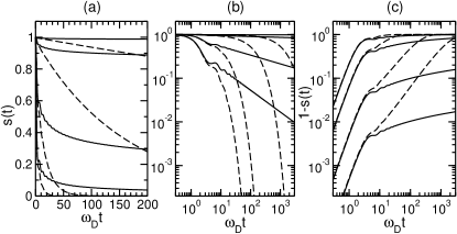
Fig. 1 illustrates the effect of the coupling strength and of finite temperature . Panels (a) and (b) display the usual long-time decay while (c) focusses on the deviation from unity. For quantum information processes Fig. 1c shows the relevant data since should be as low as possible. If error correction is to be applied thresholds between Aliferis et al. (2006); Reichardt (2006) and Knill (2004); Reichardt (2004) have to be met. Inspecting Fig. 1c we conclude that for values of of about the qubit can be stored only for tiny fractions of the correlation time . But even if is significantly smaller no storage is possible for , let alone for any time longer.
Another interesting conclusion is that low values of are favorable since they set a long time scale.222A numerical estimate yields for K a correlation time of 25 fs which is extremely fast; a low value of only K leads to 1ps which is more favorable. This means that an elastically soft environment, for instance in an organic compound with low , is better suited than a hard environment with high . This is counterintuitive, since one might have suspected that the influence of vibrations is lower when the spring constants are higher. The objection that the positive effect of a larger in a soft medium will be thwarted by a large value of the coupling will be invalidated below.
We pass now to a sequence of pulses where the total time interval is split into smaller intervals with . The -values are taken to be fixed. At each instance a -pulse is applied which effectively changes the sign of the interaction in Eq. (1). Hence the observable signal changes from in Eq. (4) to
| (7a) | |||||
| (7b) | |||||
The evaluation of is based on the same identities as the one of except that it is algebraically more involved. The result is cast in the form
| (8a) | |||||
| (8b) | |||||
| (8c) | |||||
where the factor in the integrand of the phase reads
| (9) |
and the factor in the integrand of reads
| (10) |
The phase is less harmful since its influence on the signal is only quadratic in . Hence we focus on . The procedure discussed so far is based on equidistant pulses Viola and Lloyd (1998); Ban (1998); Cappellaro et al. (2006) with yielding
| (11a) | |||||
| (11b) | |||||
For small values of these functions rise quadratically like omitting rapid oscillations. Even without performing the integrations in (8) one can read off two features: (i) a large number of pulses is advantageous. The time scale is prolonged like . (ii) no further suppression is achieved since the power law remains unchanged.
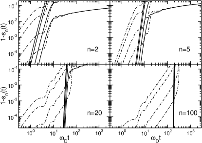
Results of the equidistant -pulse sequence are shown in Fig. 2 as dashed-dotted lines. Clearly, a shift to the right is discernible reflecting the growing factor . But no significant change of the slopes occurs. It is still important to have a weak coupling between qubit and bosonic bath to store the qubit for a significant time. For instance 100 pulses make it possible to store the qubit up to an error of for at while for it may be stored for .
Now we pose the question whether the sequence of pulses can be optimized, for instance by exploiting the freedom of choosing the instants of the pulses. The potential of non-equidistant pulse sequences was recently demonstrated by concatenated pulse sequences Khodjasteh and Lidar (2005). In our work, we aim at finding the optimum pulse sequence with respect to canonical requirements.
Inspecting (10) one realizes that always and that there are free parameters . So one may require that additional conditions are fulfilled. We use this freedom to make the first derivatives with vanish. Nicely, the resulting equations have a simple analytic solution for -pulses
| (12) |
This is the main result of this Letter. The resulting factor in the integrand yields
| (13a) | |||||
| (13b) | |||||
where the second line with the Bessel function represents a very good approximation valid for up to exponential corrections. Note that manifesting the effect of the vanishing leading derivatives. From (13) follows that the integrand stays extremely small up to a certain value of of the order of unity implying that decoherence hardly takes place up to a certain time given by . Beyond this time it sets in very abruptly.
How does our finding compare to known results? For we retrieve from Eq. 12 and . This means that our pulse sequence with the initial -pulse about and two -pulses about reproduces the CPMG-cycle Haeberlen (1976) which is widely considered for decoherence suppression Witzel and Sarma (2006); Yao et al. (2006). For all , Eq. 12 predicts so far unexplored pulse sequences with a better potential for decoherence suppression.
Fig. 2 depicts the features of the optimum sequence. Clearly, the lines are shifted to the right reflecting the factor in in parallel to the effect of equidistant pulses. In contrast to equidistant pulses the optimized pulses lead to steeper and steeper slopes on increasing implying that the behavior for different couplings becomes almost indistinguishable. This feature is extremely advantageous because it means practically that even a large coupling does not harm a long storage time. For instance for 100 pulses the qubit may be stored for independently of the value of . The possible storage time is by a factor of 40 better than for the equidistant scheme for . For the improvement is still about a factor of 4. Clearly, the improvement is most striking for large values of the coupling. Recurring to the estimate of ps endnote23 we see that 100 pulses allow us to extend the storage time to about 200ps.
Another way of looking at the optimized scheme Eq. 12 is to ask how many pulses are needed to achieve a certain storage time with an error below a certain threshold, say . For , 5 or 6 pulses already imply a storage time of . For the same storage the equidistant scheme requires about 100 pulses. Keeping in mind that in practice each pulse will be imperfect it is certainly advantageous to work with a minimum number of pulses.
Let us turn to temperature. In practice, no system will be at and in particular the favorable soft media will be operated at relative high compared to the cutoff temperature (setting ). In our model, enters in the Eqs. (6c,8c) by the factor reflecting the thermal occupation of the bosonic modes. It deviates from its value of unity only for small frequencies. Small frequencies mean small values of so that the suppression of in this range, see Eq. (13b), is particularly helpful. Finite temperature does not lead to any noticeable decoherence as long as the storage time is not too long, i.e. as long as it stays below . Indeed, curves at are indistinguishable from the solid ones in Fig. 2. This holds already for a rather small number of pulses so that it is a highly relevant feature for experimental realizations. For the equidistant scheme the thermal effects are larger, in particular for large temperatures . The extreme insensitivity to thermal effects represents another essential advantage of the optimized scheme.
The above derivations hold for arbitrary , i.e. even for the classical limit . Indeed, the same pulse sequences can be used for the classical Hamiltonian where is controlled by Gaussian fluctuations determined by and by . The Fourier transform of is the power spectrum and replaces in Eqs. (6c,8c) while the phases and are zero classically. The other equations remain the same, in particular Eqs. (12,13). This observation greatly increases the applicability of our findings since many systems, not only bosonic baths, can be described for high temperatures by classical Gaussian fluctuations.
The equidistant dynamic decoupling or iterated CPMG cycles have been realized experimentally, in particular in NMR experiments. The detrimental influence of very slow nuclear spins on a solid-state qubit Fraval et al. (2005) or on the electron spin in quantum dots Petta et al. (2005) has been reduced recently. A Rabi oscillation could be made vanish by realizing sequences of almost instantaneous -pulses exploiting the interplay between nuclear and electronic spins Morton et al. (2006). Krojanski and Suter demonstrated recently that even the decoherence of large quantum registers, realized by nuclear spins and their dipole-dipole interaction, can be significantly reduced by dynamic decoupling Krojanski and Suter (2006). To our knowledge, however, no optimized sequences obeying Eq. (12) have been examined.
An optimized sequence is by definition more efficient than a random one, cf. Ref. Viola and Knill (2005). But for large symmetry groups it may be easier to use a random scheme than to optimize the pulse sequence. If more specific information on the bath is available, cf. Ref. Yao et al. (2006), other, specifically adapted schemes might work more efficiently. Furthermore, we emphasize that hybrid techniques are attractive: Any other dynamic decoupling scheme may be improved by replacing the -pulse or the CPMG cycle of two -pulses by a suitable sequence obeying Eq. 12. The optimized design of real -pulses of finite duration in the presence of bosonic baths, cf. Ref. Möttönen et al. (2006) for classical baths, is left for future research.
In summary, we discussed strategies for suppressing the decoherence of physical quantum bits by dynamic decoupling. A promising way to optimize the sequence of -pulses beyond the well-known CPMG sequence was analytically established. The comparison to equidistant pulse sequences revealed that the optimized scheme enhances the possible storage time by up to almost two orders of magnitude. Alternatively, the number of pulses required to achieve a certain prolongation of the storage time can be much smaller (by a factor of 20 for strong coupling to the bosonic bath) than for the standard equidistant scheme. Additionally, the optimized scheme is extremely insensitive to detrimental thermal fluctuations. So experimental investigations of the optimized scheme are called for.
Acknowledgements.
I like to thank F.B. Anders, S. Pasini, C. Raas, J. Stolze, and D. Suter for helpful discussions.References
- Zoller et al. (2005) P. Zoller, T. Beth, D. Binosi, R. Blatt, H. Briegel, D. Bruss, T. Calarco, J. I. Cirac, D. Deutsch, J. Eisert, et al., Eur. Phys. J. D 36, 203 (2005).
- Viola and Lloyd (1998) L. Viola and S. Lloyd, Phys. Rev. A 58, 2733 (1998).
- Ban (1998) M. Ban, J. Mod. Opt. 45, 2315 (1998).
- Facchi et al. (2005) P. Facchi, S. Tasaki, S. Pascazio, H. Nakazato, A. Tokuse, and D. A. Lidar, Phys. Rev. A 71, 022302 (2005).
- Cappellaro et al. (2006) P. Cappellaro, J. S. Hodges, T. F. Havel, and D. G. Cory, J. Chem. Phys. 125, 044514 (2006).
- Haeberlen (1976) U. Haeberlen, High Resolution NMR in Solids: Selective Averaging (Academic Press, New York, 1976).
- Witzel and Sarma (2006) W. M. Witzel and S. D. Sarma, cond-mat/0604577 (2006).
- Leggett et al. (1987) A. J. Leggett, S. Chakravarty, A. T. Dorsey, M. P. A. Fisher, A. Garg, and W. Zwerger, Rev. Mod. Phys. 59, 1 (1987).
- Weiss (1999) U. Weiss, Quantum Dissipative Systems (World Scientific, Singapore, 1999), 2nd ed.
- Aliferis et al. (2006) P. Aliferis, D. Gottesman, and J. Preskill, Quant. Inf. Comput. 6, 97 (2006).
- Reichardt (2006) B. W. Reichardt, in Lecture Notes in Computer Science (Springer, Berlin/Heidelberg, 2006), vol. 4051, p. 50.
- Knill (2004) E. Knill, quant-ph/0404104 (2004).
- Reichardt (2004) B. W. Reichardt, quant-phys/0406025 (2004).
- Khodjasteh and Lidar (2005) K. Khodjasteh and D. A. Lidar, Phys. Rev. Lett. 95, 180501 (2005).
- Yao et al. (2006) W. Yao, R. Liu, and L. J. Sham, cond-mat/0604634 (2006).
- Fraval et al. (2005) E. Fraval, M. J. Sellars, and J. J. Longdell, Phys. Rev. Lett. 95, 030506 (2005).
- Petta et al. (2005) J. R. Petta, A. C. Johnson, J. M. Taylor, E. A. Laird, A. Yacoby, M. D. Lukin, C. M. Markus, M. P. Hanson, and A. C. Gossard, Science 309, 2180 (2005).
- Morton et al. (2006) J. J. L. Morton, A. M. Tyryshkin, A. Ardavan, S. C. Benjamin, K. Porfyrakis, S. A. Lyon, and G. A. D. Briggs, Nature Phys. 2, 40 (2006).
- Krojanski and Suter (2006) H. G. Krojanski and D. Suter, Phys. Rev. Lett. 97, 150503 (2006).
- Viola and Knill (2005) L. Viola and E. Knill, Phys. Rev. Lett. 94, 060502 (2005).
- Möttönen et al. (2006) M. Möttönen, R. de Sousa, J. Zhang, and K. B. Whaley, Phys. Rev. A 73, 022332 (2006).