Quantum limits in image processing

Abstract

We determine the bound to the maximum achievable sensitivity in the estimation of a scalar parameter from the information contained in an optical image in the presence of quantum noise. This limit, based on the Cramer-Rao bound, is valid for any image processing protocol. It is calculated both in the case of a shot noise limited image and of a non-classical illumination. We also give practical experimental implementations allowing us to reach this absolute limit.

Introduction. - Many of the most sensitive techniques for the measurement of a physical parameter - which we will call $p$ in the following and assume to be a scalar - are optical. In some cases, the total intensity or amplitude of the light beam varies with $p$ and conveys the information. It is then well known Kimble ; Fabre ; Gao ; SQL that there exists a standard quantum limit in the sensitivity of the measurement of $p$ when the light beam is in a coherent state, and that it is possible to go beyond this limit using sub-Poissonian or squeezed light. In other cases, the parameter $p$ of interest only modifies the distribution of light in the transverse plane and not its total intensity. The present paper deals with this latter situation. For example, the parameter $p$ modifies the position or direction of a light beam. This configuration has been studied at the quantum level, both theoretically and experimentally using split detectors displacement11 ; displacement12 ; displacement13 or homodyne detection Delaubert2006 ; displacement21 . But in many instances the parameter $p$ affects in a complicated way the field distribution in the detection plane (that we will call here the image). For example a fluorescent nano-object imbedded in a biological environment modifies the image recorded through a microscope in a complex way because of diffraction. Nevertheless its position can be determined from the information contained in the image with a sensitivity which can be much better than the wavelength nano . In order to extract the parameter value in such experiments, one needs to use detector arrays or CCD cameras and to combine in an appropriate way the information recorded on the different pixels.

When all the sources of technical noise have been removed in the apparatus, quantum fluctuations still affect the optical measurement and limit its sensitivity, in a way that can be readily calculated for each specific measurement protocol. The purpose of this paper is much broader. It is to answer the following question: what is the lowest limit imposed by quantum noise to the accuracy of the determination of $p$, independently of the information processing protocol used for the extraction of information? As we will see, this optimum limit depends only on the statistics of the fluctuations of the incoming light. We use an approach based on the Cramer-Rao Bound. This tool, widely used in the signal processing community Refregier2002 , has already been applied to different domains, such as gravitational wave detection Nicholson or diamagnetism Curilef .

Notations and assumptions. - The parameter $p$ is measured relative to an a priori value chosen for simplicity to be $0$. Because of the quantum fluctuations in the optical measurements, there will be an uncertainty on its estimation. An evaluation of this uncertainty thus provides the precision on the determination of the parameter $p$ around a zero value.

The mean value of the local complex electric field operator in the image plane, normalized to a number of photons, will be written for a given value of the parameter as

$$\bar{E}(\vec{r},p)=2\sqrt{N}u_{0}(\vec{r},p),$$ (1)

where $N$ refers to the total number of photons detected in the mean field during the integration time of the detector. $N$ is assumed to be independent of $p$, as stated previously. $u_{0}(\vec{r},p)$ is the $p$-dependent transverse distribution of the mean field, complex in the general case, and normalized to $1$ (its square modulus integrated over the transverse plane equals 1). The local mean photon number detected during the same time interval is

$$\bar{n}(\vec{r},p)=\frac{\bar{E}^{*}(\vec{r},p)\bar{E}(\vec{r},p)}{4}=N|u_{0}(\vec{r},p)|^{2}.$$ (2)

Intensity measurements. - We first assume that $p$ is determined by processing the information contained in the measurement of the local intensity, i.e. local number of photons. The best possible local intensity detection device would consist in a set of indexed pixels paving the entire transverse plane, in the limit when their spatial extension approaches $0$. Let $\textbf{n}=\left[n_{1},...,n_{k},...\right]$ be one measurement of the photon distribution with such a hypothetical detector, where $n_{k}$ corresponds to the number of photons detected on pixel $k$. Because of the noise present in the light, the sample n differs from its statistical mean value $\bar{\textbf{n}}(p)=\left[\bar{n}_{1}(p),...,\bar{n}_{k}(p),...\right]$. Let $L(\textbf{n}|p)$ be the likelihood of its observation. Note that n corresponds to a single measurement and hence does not explicitly depend on $p$, contrarily to the average on all the possible realizations.

The achievable precision on the estimation of $p$ is limited by the Cramer-Rao Bound (CRB). More precisely, the variance of any unbiased estimator of $p$ is necessarily greater than $\sigma_{min}^{2}=1/I_{F}$, where the Fisher information $I_{F}$ is given, when the actual value of $p$ is $0$, by Refregier2002 :

$$I_{F}=-\int\left.\frac{\partial^{2}}{\partial p^{2}}l(\textbf{n}|p)\right|_{p=0}L(\textbf{n}|0)d\textbf{n},$$ (3)

where we have introduced the log-likelihood $l(\textbf{n}|p)=\ln{L(\textbf{n}|p)}$. The integration spans continuously over all possible photon distributions that can be detected when the parameter value is $p=0$. This information is thus highly dependent on the noise statistics.

Let us first assume that the illumination is coherent, and therefore that the local intensity noise is Poissonian. The probability of measuring $n_{k}$ photons on pixel $k$, when the parameter equals $p$ is given by

$$P_{k,p}(n_{k})=\frac{\bar{n}_{k}(p)^{n_{k}}}{n_{k}!}e^{-\bar{n}_{k}(p)}.$$ (4)

Restricting our analysis to spatially uncorrelated beams, the likelihood $L(\textbf{n}|p)$ simply corresponds to the product of all local probabilities given in Eq. 4. Then, taking the limit of infinitely small pixels and using Eq. 3, one can show that the Fisher information equals

$$I_{F}^{Poisson}=\int\left[\frac{\bar{n}^{\prime}(\vec{r},0)^{2}}{\bar{n}(\vec{r},0)}-\bar{n}^{\prime\prime}(\vec{r},0)\right]d^{2}r,$$ (5)

where the ^′ denotes a derivative relative to $p$. Using Eq. 1, one finally finds that

$$I_{F}^{Poisson}=\frac{4N}{a^{2}},$$ (6)

where $a$ is a global positive parameter characterizing the variation of the image intensity with $p$, defined by

$$\frac{1}{a^{2}}=\int\left[\frac{\partial}{\partial p}|u_{0}(\vec{r},p)|\right]_{p=0}^{2}d^{2}r.$$ (7)

The smallest value of $p$ that can be distinguished from the shot noise - i.e. corresponding to a signal to noise ratio (SNR) equal to 1 -, whatever the algorithm used to determine it from the local intensity measurements, provided that it gives an unbiased estimation of $p$, is finally greater than $a/2\sqrt{N}$. This value sets the standard quantum noise limit for intensity measurements of $p$, imposed by the random time arrival of photons on the detector. It is inversely proportional to the square root of the number of photons, as expected, and is related, through the dependence with $a$, to the modification of the mean intensity profile with $p$.

We now consider a non-classical illumination, still with identical mean intensity, but with local sub-Poissonian quantum fluctuations described by a noise variance $\sigma_{P}^{2}~{}<~{}1$ (assumed to be the same over the entire transverse plane). One can show that the CRB leads to

$$p_{min}^{sub-Poisson}\geq\frac{a\sigma_{P}}{2\sqrt{N}}.$$ (8)

As we have already noticed, the limit given by Eq. 8 is valid for any measurement strategy. Nevertheless, a practical way enabling us to reach such an absolute limit remains to be found. This is what is presented in the next paragraph.

Let us assume that an image processor calculates a given linear combination of the local intensity values recorded by the pixels of an array detector, as represented in Fig. 1.

Figure 1: Array detector as an optimal intensity detection. $g$ refers to the pixel gain distribution. $S(p)$ is the p-dependent processed signal.

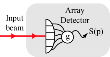
Assuming that the pixels are small compared to the characteristic variation length of the image, the mean value $\bar{S}(p)$ of the computed signal can be written as an integral over the transverse plane as follows

$$\bar{S}(p)=\int g(\vec{r})\bar{n}(\vec{r},p)d^{2}r,$$ (9)

where $g(\vec{r})$ is the local gain on the pixel localized at position $\vec{r}$, which can be positive or negative. Assuming that $p$ is small, $|u_{0}(\vec{r},p)|$ can be expanded at first order into

$$|u_{0}(\vec{r},p)|=|u_{0}(\vec{r},0)|+\frac{p}{a}u_{I}(\vec{r}),$$ (10)

where $a$ has been defined in Eq. 7, and $u_{I}$ is a transverse function normalized to $1$, already introduced in a particular case in reference Delaubert2006 . The gains are chosen such as $\bar{S}(p=0)=0$ (difference measurement), so that $\bar{S}(p)$ is given, at first order, by

$$\bar{S}(p)=\frac{2Np}{a}\int g(\vec{r})|u_{0}(\vec{r},0)|u_{I}(\vec{r})d^{2}r,$$ (11)

For a coherent illumination, because the local quantum fluctuations are uncorrelated, the noise variance $\Delta S^{2}$ on on $\bar{S}(p)$ is equal to the shot noise on each pixel weighted by $g^{2}(\vec{r})$ Treps2005 . Moreover, as $p$ is small, the noise is independent of $p$ at the first order, and we get

$$\Delta S^{2}=N\int g^{2}(\vec{r})|u_{0}(\vec{r},0)|^{2}d^{2}r.$$ (12)

It is then possible to optimize the gain factor $g(\vec{r})$ in order to get the highest possible SNR defined by SNR$=\bar{S}(p)^{2}/\Delta S^{2}$. Using Cauchy-Schwartz inequality, one can show that the highest SNR value for the present measurement strategy is given by SNR$=4Np^{2}/a^{2}$, and is obtained for an optimal value of the gain distribution given by

$$g_{opt}(\vec{r})=\beta\frac{u_{I}(\vec{r})}{|u_{0}(\vec{r},0)|},$$ (13)

where $\beta$ is an arbitrary constant. The minimum measurable value of $p$ - corresponding to comparable signal and noise, i.e. SNR$=1$ - is given by $p_{min}=a/2\sqrt{N}$, which is precisely equal to the CRB for classical illumination. The present measurement strategy is therefore optimal as it allows to reach the CRB for small values of the parameter $p$, with the certainty that no other measurement strategy can do better. Note that we have not proven that it is the unique way to reach the CRB.

We can even extend this result to the use of non classical light. Indeed, using a bimodal field composed of a bright mode $u_{0}$ in a coherent state carrying the mean field, and a squeezed vacuum mode in the mode $u_{I}$, the detected noise power is modified into

$$\Delta S^{2}=N\sigma_{P}^{2},$$ (14)

when the noise variance on the amplitude quadrature of the mode $u_{I}$ is given by $\sigma_{P}^{2}$ Treps2005 . Note that the use of a locally squeezed beam would not provide any improvement as $u_{I}$ is the only mode contributing to the measurement noise, referred to as the noise-mode of detection Delaubert2006 ; Treps2005 . The minimum measurable $p$ value is in this case

$$p_{min}=\frac{a\sigma_{P}}{2\sqrt{N}}.$$ (15)

We have thus found a way to reach the bound, i.e. the minimum accessible $p$-value given in Eq.8. Moreover, our scheme requires minimum quantum resources, namely a bimodal field with squeezing in only one mode.

Field measurements. - We now assume that the information about $p$ is extracted from the knowledge of the local complex field, i.e. local amplitude and phase, that can be obtained by interferometric techniques. Similarly to the previous section, the best possible detection would here access the local complex field on k-indexed areas paving the entire transverse plane, in the limit when their spatial extension approaches $0$. Let $\textbf{E}=\left[E_{1},...,E_{k},...\right]$ be a single measurement of the field distribution, hence independent of $p$, where $E_{k}$ corresponds to the complex field detected on area $k$. Again, because of the noise present in the light, the sample E differs from its statistical mean value $\bar{\textbf{E}}(p)=\left[\bar{E}_{1}(p),...,\bar{E}_{k}(p),...\right]$. Let $L(\textbf{E}|p)$ be the likelihood of its observation.

A bound to the maximal precision on $p$ can again be calculated from the CRB, which, for a field measurement, is the inverse of the following Fisher information

$$I_{F}=-\int\left[\frac{\partial^{2}}{\partial p^{2}}l(\textbf{E}|p)\right]_{p=0}L(\textbf{E}|0)d\textbf{E},$$ (16)

We assume that the local field fluctuations in the transverse plane can be described by a Gaussian probability density function independent of the mean field. Moreover, we consider a classical or non classical illumination whose amplitude and phase quadrature fluctuations are described by the noise variances $\sigma_{P}^{2}$ and $\sigma_{Q}^{2}$, respectively. These factors neither depend on $\vec{r}$ nor on $p$, as we assume the fluctuations to be homogeneous and independent of the parameter $p$.

The probability to measure a field given by $E_{k}=P_{k}+iQ_{k}$ on area $k$, where $P_{k}$ and $Q_{k}$ correspond to the local field quadratures, is, for a parameter value $p$

$$\mathcal{P}_{k,p}(E_{k})=\frac{1}{2\pi\sigma_{P}\sigma_{Q}}e^{-\left[\frac{\left(P_{k}-\bar{P}_{k}(p)\right)^{2}}{2\sigma_{P}^{2}}+\frac{\left(Q_{k}-\bar{Q}_{k}(p)\right)^{2}}{2\sigma_{Q}^{2}}\right]},$$ (17)

where $\bar{P}_{k}(p)$ and $\bar{Q}_{k}(p)$ are the local quadratures statistical averages, satisfying: $\bar{E}_{k}(p)=\bar{P}_{k}(p)+i\bar{Q}_{k}(p)$. Without loss of generality, we define the orientation of the Fresnel diagram relative to the phase of the mean field, i.e. $\bar{P}(\vec{r},p)=2\sqrt{N}u_{0}(\vec{r},p)$ and $\bar{Q}(\vec{r},p)=0$, taking the limit of infinitely small detection areas. Assuming no spatial correlations in the field fluctuations, one can show that the Fisher information is given by

$$I_{F}^{Gauss} = \int\frac{1}{\sigma_{P}^{2}}\left[\frac{\partial\bar{P}(\vec{r},p)}{\partial p}\right]^{2}_{p=0}d^{2}r.$$ (18)

We now introduce $b$, a second global positive parameter, characterizing the variation of the image field with $p$

$$\frac{1}{b^{2}}=\int\left[\frac{\partial}{\partial p}u_{0}(\vec{r},p)\right]_{p=0}^{2}d^{2}r.$$ (19)

Using Eq.1 and 19, the Fisher information simplifies into

$$I_{F}^{Gauss}=\frac{4N}{b^{2}\sigma_{P}^{2}}.$$ (20)

The smallest value of $p$ that can be distinguished from the quantum noise using a field detection of the optical beam is finally greater than the CRB:

$$p_{min}^{Gauss}\geq\frac{b\sigma_{P}}{2\sqrt{N}}.$$ (21)

Again, we can propose an experimental scheme enabling to reach this limit in the case of a small parameter $p$, and for which the mean value of the complex electric field can be written at first order

$$\bar{E}(\vec{r},p)=2\sqrt{N}\left[u_{0}(\vec{r},0)+\frac{p}{b}u_{E}(\vec{r})\right],$$ (22)

where $b$ has been introduced in Eq.19, and where $u_{E}(\vec{r})$ is a transverse function normalized to $1$.

Let us consider a balanced homodyne detection, as represented in Fig. 2, with a local oscillator (LO) chosen to be defined by the following complex field operator

$$\bar{E}_{LO}(\vec{r})=2\sqrt{N_{LO}}u_{E}(\vec{r})e^{i\theta_{LO}},$$ (23)

where $N_{LO}$ corresponds to the number of photons detected in the entire LO beam during the integration time.

Figure 2: Balanced homodyne detection as an optimal field detection. $n_{-}(p)$ is the p-dependent signal. $\phi_{LO}$ is the local oscillator phase. BS : $50/50$ beamsplitter.

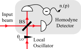
The LO is much more intense than the image, i.e. $N_{LO}\gg N$. $\theta_{LO}$ is the LO phase. The mean intensity difference $n_{-}$ between the photocurrents of the two detectors is given in terms of number of photons by

$$\bar{n}_{-}(p)=\frac{1}{4}\int\left[\bar{E}^{*}_{LO}(\vec{r})\bar{E}(\vec{r},p)+\bar{E}^{*}(\vec{r},p)\bar{E}_{LO}(\vec{r})\right]d^{2}r.$$ (24)

Note the similarity with Eq.9, as incident field amplitude and LO field play here identical roles of incident intensity and electronic gain, respectively. Though detectors do not resolve the spatial distribution of the beams and no processing of the spatial information is made, the balanced homodyne technique directly provides an ”analog” computation of the quantity of interest.

When the LO phase is tuned to the maximum of the $p$-dependent term, the homodyne signal becomes

$$\bar{n}_{-}=2\sqrt{NN_{LO}}\frac{p}{b}.$$ (25)

For coherent illumination, the noise power on the homodyne signal corresponds to $N_{LO}$, i.e. to the shot noise of the LO. The SNR of the homodyne measurement is thus given by SNR$=4Np^{2}/b^{2}$. The minimum measurable value of $p$ - corresponding to a SNR of $1$ - with homodyne detection is given by

$$p_{min}=\frac{b}{2\sqrt{N}}.$$ (26)

Moreover, when the component of the image selected by the LO is in a non classical state , i.e. allowing a squeezed vacuum $u_{E}$ mode with a noise variance $\sigma_{P}^{2}$ on the amplitude quadrature within the incoming beam, we get

$$p_{min}=\frac{b\sigma_{P}}{2\sqrt{N}}.$$ (27)

This result corresponds exactly to the CRB calculated for amplitude measurements of $p$. The homodyne detection scheme with the appropriate LO shape and phase is therefore an optimal field detection of $p$. Again, it uses minimal resources as only one source of squeezed light is needed to reach the non classical CRB.

Comparison and conclusion. - We have presented two efficient - i.e. reaching the associated CRB - signal processing techniques for the extraction of information contained in an image. We can show that the CRB for field measurements, in which all quadratures can be accessed, is smaller than the one for intensity measurements, i.e. $a\geq b$. Yet, both schemes are useful: the intensity scheme is interesting since it is not restricted to monochromatic light, whereas the amplitude scheme is useful since it does not require pixellized detectors.

Let us finally note that this work provides limits which are valid for a shot noise limited light of any shape. However it is not valid so far for any kind of non-classical light, as we have restricted our analysis to homogeneous squeezed states. In a forthcoming publication, we will study the situation of quantum fields with quantum spatial correlations in the transverse plane and will investigate for the corresponding modifications of the CRB.

Acknowledgements. We would like to acknowledge the support of the Australian Research Council scheme for Centre of Excellence. Laboratoire Kastler Brossel, of the Ecole Normale Supérieure and Université Pierre et Marie Curie, is associated with the CNRS.

References

- (1) M. Xiao et al., Phys. Rev. Lett. 59, 278 (1987).
- (2) P. H. Souto Ribeiro et al., Opt. Lett. 22, 1893 (1997).
- (3) J. Gao et al., Opt. Lett. 23, 870 (1998).
- (4) H.A. Bachor et al., A guide to experiments in quantum optics, Wiley-VCH (2003).
- (5) C. Fabre et al., Opt. Lett.25, 76 (2000).
- (6) N. Treps et al., Phys. Rev. Lett. 88 203601 (2002)
- (7) N. Treps et al., Science, 301, 940 (2003).
- (8) V. Delaubert et al., Opt. Let. 31, 1537 (2006)
- (9) V. Delaubert et al., preprint quant-ph/0607142.
- (10) A. Rohrbach et al., Rev. Sci. Instrum. 75, 2197 (2004)
- (11) P. Réfrégier, Noise Theory and Application to Physics, Springer, New-York, (2004).
- (12) D. Nicholson et al., Phys. Rev. D 57, 4588 (1998).
- (13) S. Curilef et al., Phys. Rev. B, 71, 024420 (2005).
- (14) N. Treps et al., Phys. Rev. A 71, 013820 (2005).