Generalized Limits for Single-Parameter Quantum Estimation

Abstract

We develop generalized bounds for quantum single-parameter estimation problems for which the coupling to the parameter is described by intrinsic multi-system interactions. For a Hamiltonian with $k$-system parameter-sensitive terms, the quantum limit scales as $1/N^{k}$ where $N$ is the number of systems. These quantum limits remain valid when the Hamiltonian is augmented by any parameter-independent interaction among the systems and when adaptive measurements via parameter-independent coupling to ancillas are allowed.

Many problems that lie at the interface between physics and information science can be addressed using techniques from parameter estimation theory. Precision metrology, timekeeping, and communication offer prominent examples; the parameter of interest might be the strength of an external field, the evolved phase of a clock, or a communication symbol. Fundamentally, single-parameter estimation is a quantum-mechanical problem: one must infer the value of a coupling constant $\gamma$ in the Hamiltonian $H_{\gamma}=\hbar\gamma h_{0}$ of a probe system by observing the evolution of the probe due to $H_{\gamma}$ Helstrom (1976); Holevo (1982); Braunstein and Caves (1994); Braunstein et al. (1996); Giovannetti et al. (2006). We take $\gamma$ to have units of frequency, thus making $h_{0}$ a dimensionless coupling Hamiltonian.

Quantum mechanics places limits on the precision with which $\gamma$ can be determined. It is now well established, via the quantum Cramér-Rao bound Helstrom (1976); Holevo (1982); Braunstein and Caves (1994); Braunstein et al. (1996), that the optimal uncertainty in any single-parameter quantum estimation procedure is $\delta\gamma\sim 1/\sqrt{\nu}\,t\,\Delta h_{0}$, where $\nu$ is the number of independent probes used, $t$ is the evolution time of each probe, and $\Delta h_{0}$ is the standard deviation (uncertainty) of $h_{0}$ Braunstein and Caves (1994); Braunstein et al. (1996). The $1/\sqrt{\nu}$ dependence is the standard statistical improvement with number of trials; generally, for nonGaussian statistics, the sensitivity $1/\sqrt{\nu}\,t\,\Delta h_{0}$ can only be attained asymptotically for a large number of trials. Besides increasing the number of trials, there are two other obvious ways to improve the sensitivity: (i) the probe can be allowed to evolve under $H_{\gamma}$ for a longer time $t$; (ii) the quantum state of the probe can be chosen to maximize the deviation $\Delta h_{0}$. In all practical settings, decoherence or other processes limit the useful interaction time; in addition, temporal fluctuations in $\gamma$ often prevent the evolution time from being arbitrarily extended. For a given parameter estimation problem, $h_{0}$ is fixed, as is its maximum deviation.

Quantum mechanics does, however, provide another opportunity: gathering $N$ probe systems into a single probe, which is prepared in an appropriate entangled state; if $\Delta h_{0}$ for the entangled state increases faster than $\sqrt{N}$, the sensitivity improves, provided there is still a sufficient number of probes to reach the asymptotic regime in number of trials. This Letter focuses on how $\delta\gamma$ scales with $N$, the number of systems in a probe. Thus we work throughout with bounds on the sensitivity of a single probe, remembering that the bounds can only be achieved by averaging over many probes, but preferring not to muddy the discussion by carrying along the $1/\sqrt{\nu}$ dependence on the number of probes.

For the $N$ systems in a probe, it has been traditional to consider Hamiltonians of the form

$$H_{\gamma}=\hbar\gamma h_{0}\;,\qquad h_{0}=\sum_{j=1}^{N}h_{j}\;,$$ (1)

where the $h_{j}$’s are single-system dimensionless coupling Hamiltonians, assumed to be identical. Restriction to Hamiltonians that are separable and invariant under particle exchange, as in Eq. (1), is physically motivated: in metrology it is generally desirable to make the coupling to the parameter homogeneous, and multi-body effects are typically undesirable because they are less well characterized. In atomic clocks, for instance, much experimental effort is directed toward achieving a Hamiltonian of the form (1). In many cases, even the measurements performed on the probe are unable to distinguish between individual constituents.

To determine how the optimal parameter uncertainty scales with $N$, one maximizes the deviation $\Delta h_{0}$ over joint states of the probe systems. If entanglement is not allowed, the probe systems can be regarded themselves as independent probes; in this case, $\Delta h_{0}$ scales as $\sqrt{N}$, producing the so-called shot-noise limit found in precision magnetometry, gravimetry, and timekeeping Wineland et al. (1994). When entanglement is allowed, however, one can choose the initial probe state to be the “cat state,”

$${1\over\sqrt{2}}\Bigl{(}|\lambda_{M},\ldots,\lambda_{M}\rangle+|\lambda_{m},\ldots,\lambda_{m}\rangle\Bigl{)}\;,$$ (2)

where for system $j$, $|\lambda_{M}\rangle$ ($|\lambda_{m}\rangle$) is the eigenstate of $h_{j}$ with maximum (minimum) eigenvalue $\lambda_{M}$ ($\lambda_{m}$). This yields a deviation $\Delta h_{0}=N(\lambda_{M}-\lambda_{m})/2$ that scales linearly in $N$ Braunstein and Caves (1994); Giovannetti et al. (2006), a scaling known as the Heisenberg limit. Evolution under $H_{\gamma}$ for time $t$ introduces a relative phase $e^{i\phi(t)}$ into the cat state, with $\phi(t)=\gamma tN(\lambda_{M}-\lambda_{m})$, and leaves $\Delta h_{0}$ unchanged; the Heisenberg limit can be attained (asymptotically for many trials) by measuring on each probe system an observable two of whose eigenvectors are $|\pm\rangle=(|\lambda_{M}\rangle\pm|\lambda_{m}\rangle)/\sqrt{2}$.

The Heisenberg limit is not general since there are physical systems of interest for parameter estimation where a coupling Hamiltonian of the form (1) is overly restrictive. In particular, some condensed and even quantum-optical systems exhibit nonlinear collective effects due to multi-body or tensor-field interactions Botet et al. (1982); Cirac et al. (1998); You et al. (2006). In such systems, multi-body terms in the Hamiltonian can couple to metrologically relevant parameters. In this Letter we generalize single-parameter quantum estimation to intrinsic many-body interactions, which surpass the conventional Heisenberg limit. Our work is largely inspired by a recent paper of Roy and Braunstein Roy and Braunstein (2006), which claimed an exponential scaling for a collection of $N$ qubits with a particular Hamiltonian. We argue below that the exponential scaling is unphysical.

We turn now to showing that Hamiltonians with intrinsic $k$-body terms generate a family of parameter estimation problems, characterized by $k$, where the quantum limit scales as $1/N^{k}$. For this purpose, we consider Hamiltonians of the form

$$H_{\gamma}(t)=\hbar\gamma h_{0}+\tilde{H}(t)\;,\quad h_{0}=\sum_{\{j_{1},\ldots,j_{k}\}}h_{j_{1},\ldots,j_{k}}^{(k)}\;,$$ (3)

where $h_{0}$ is the dimensionless Hamiltonian that describes coupling to the parameter. The auxiliary Hamiltonian $\tilde{H}(t)$ is discussed below. In $h_{0}$, $k$ denotes the degree of multi-body coupling, with the sum running over all subsets of $k$ systems. We could also include couplings of different degrees up to a maximum degree, but since the maximum degree dominates the sensitivity scaling, we stick with a single degree $k$ in the following. We assume that the $k$-body coupling $h^{(k)}$ is symmetric under exchange of probe systems. Moreover, we assume that $k$ and $h^{(k)}$ are independent of the number of probe systems. We make this latter assumption, that $h_{0}$ is an intensive property of the probe, because we want to consider a particular kind of coupling to the parameter which remains unchanged as $N$ changes. For real physical systems, the symmetry and intensive assumptions will hold only approximately and only over some range of values of $N$.

The auxiliary Hamiltonian $\tilde{H}(t)$ includes all parameter-independent contributions to $H_{\gamma}$. For example, it includes the free Hamiltonians of the probe systems and any parameter-independent interactions among them. In addition, we can introduce an undetermined number of ancillas and let $\tilde{H}$ include the couplings of the ancillas to the probe systems and any couplings among the ancillas. Measurements on the ancillas can be included as part of an overall final measurement on the probe-ancilla system; since the Cramér-Rao bound that underlies our analysis holds for all possible measurements and ways of estimating $\gamma$ from the measurement results, the bounds we derive hold for arbitrary measurements on the ancillas. This conclusion applies even to measurements on the ancillas that are carried out during the evolution time and whose results are used to condition measurements on other ancillas or to control the coupling of other ancillas to the probe. By the principle of deferred measurement Nielsen and Chuang (2000), which is illustrated in Fig. 1, all such measurements can be shuffled to the end of the evolution time by making appropriate adjustments to $\tilde{H}$.

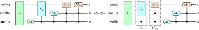
Figure 1: Quantum-circuit diagrams illustrating the principle of deferred measurement. In the circuit on the left, a measurement $M$ on the lower ancilla yields result $a$; this result controls a subsequent unitary $U_{a}$, applied to the probe and the upper ancilla, and determines a conditional measurement $M_{a}$ on the upper ancilla, which has result $b$. The two measurement results then control a unitary $U_{a,b}$ applied to the probe and a conditional measurement $M_{a,b}$ on the probe. The left-hand circuit is equivalent to the circuit on the right, in which the controls are applied coherently (boxed gates $U_{A}$ and $U_{A,B}$) and the measurements, deferred to the end of the circuit, tell one which unitary was applied. Without loss of generality, we can assume the measurements are described by orthogonal projectors $P_{a}$, $P_{b|a}$, and $P_{c|a,b}$, because any generalized measurement can be modeled by a projection-valued measurement on an extended system. The unitary transformations in the left-hand circuit, $U_{a}$ and $U_{a,b}$, are evolution operators generated by the Hamiltonians $\hbar\gamma h_{0}+\tilde{H}_{a}(t)$ and $\hbar\gamma h_{0}+\tilde{H}_{a,b}(t)$, whereas the corresponding coherent controlled unitaries in the circuit on the right, $U_{A}$ and $U_{A,B}$, are generated by the Hamiltonians $\hbar\gamma h_{0}+\sum_{a}\tilde{H}_{a}(t)\otimes P_{a}$ and $\hbar\gamma h_{0}+\sum_{a,b}\tilde{H}_{a,b}(t)\otimes P_{b|a}P_{a}$. It is easy to verify from the evolution equations that the controlled unitaries in the right-hand circuit are given by $U_{A}=\sum_{a}U_{a}\otimes P_{a}$ and $U_{A,B}=\sum_{a,b}U_{a,b}\otimes P_{b|a}P_{a}$. Thus the principle of deferred measurement can be rendered algebraically in the following way: if we use the left-hand circuit, the probability for obtaining results $a$, $b$, and $c$ takes the form $\mbox{tr}(C_{a,b,c}\rho_{0}C^{\dagger}_{a,b,c})$, where $\rho_{0}$ is the initial state of the probe and ancillas and $C_{a,b,c}=P_{c|a,b}U_{a,b}P_{b|a}U_{a}P_{a}U$; pulling the measurement projectors to the left in $C_{a,b,c}$ changes the unitaries to the corresponding coherent controlled operations, i.e., $C_{a,b,c}=P_{c|a,b}P_{b|a}P_{a}U_{A,B}U_{A}U$, which gives the form of the probability obtained from the right-hand circuit.

Now let $\rho_{0}$ be the initial state of the probe and any ancillas. After a time $t$, the state evolves to $\rho_{\gamma}(t)=U_{\gamma}(t)\rho_{0}U^{\dagger}_{\gamma}(t)$, where the evolution operator is generated by the Hamiltonian (3):

$$i\hbar{\partial U_{\gamma}(t)\over\partial t}=H_{\gamma}(t)U_{\gamma}(t)\;.$$ (4)

At time $t$, measurements are made on the probe and ancillas, the results of which are used to make an estimate $\gamma_{\rm est}$ of the parameter. The appropriate statistical measure of the estimate’s precision is the units-corrected mean-square deviation of $\gamma_{\rm est}$ from $\gamma$ Braunstein and Caves (1994); Braunstein et al. (1996):

$$\delta^{2}\gamma=\biggl{\langle}\biggl{(}{\gamma_{\rm est}\over|d\langle\gamma_{\rm est}\rangle/d\gamma|}-\gamma\biggr{)}^{\!2}\biggr{\rangle}\;.$$ (5)

Here and below expectation values are evaluated with respect to $\rho_{\gamma}(t)$.

The quantum Cramér-Rao bound states that Helstrom (1976); Holevo (1982); Braunstein and Caves (1994); Braunstein et al. (1996)

$$\delta^{2}\gamma\geq{1\over\mathcal{I}_{\gamma}(t)}\;,\quad\mathcal{I}_{\gamma}(t)=\mbox{tr}{\bigl{(}\rho_{\gamma}(t)\mathfrak{L}_{\gamma}^{2}(t)\bigr{)}}=\langle\mathfrak{L}^{2}_{\gamma}(t)\rangle\;,$$ (6)

where $\mathcal{I}_{\gamma}(t)$ is the quantum Fisher information. The Hermitian operator $\mathfrak{L}_{\gamma}(t)$, called the symmetric logarithmic derivative, is defined (implicitly) by

$$\frac{1}{2}(\mathfrak{L}_{\gamma}\rho_{\gamma}+\rho_{\gamma}\mathfrak{L}_{\gamma})=\frac{\partial\rho_{\gamma}}{\partial\gamma}=-i[K_{\gamma},\rho_{\gamma}]\;.$$ (7)

Here

$$K_{\gamma}(t)=i\frac{\partial U_{\gamma}(t)}{\partial\gamma}U^{\dagger}_{\gamma}(t)$$ (8)

is the Hermitian generator of displacements in $\gamma$. If there is no auxiliary Hamiltonian, $K_{\gamma}(t)=th_{0}$.

For pure states, differentiating $\rho_{\gamma}=\rho_{\gamma}^{2}$ shows that

$$\mathfrak{L}_{\gamma}(t)=2\frac{\partial\rho_{\gamma}(t)}{\partial\gamma}=-2i[K_{\gamma}(t),\rho_{\gamma}(t)]\;.$$ (9)

Then the Fisher information reduces to a multiple of the variance of $K_{\gamma}(t)$:

$$\mathcal{I}_{\gamma}(t)=4\bigl{(}\langle K_{\gamma}^{2}(t)\rangle-\langle K_{\gamma}(t)\rangle^{2}\bigr{)}=4\Delta^{2}K_{\gamma}(t)\;.$$ (10)

For mixed states, the variance provides an upper bound on the Fisher information, instead of equality Braunstein et al. (1996).

We define the operator semi-norm $\|H\|$ of a Hermitian operator $H$ as $\|H\|=M_{H}-m_{H}$, where $M_{H}$ ($m_{H}$) is the maximum (minimum) eigenvalue of $H$. This semi-norm is invariant under unitary transformations and obeys the triangle inequality, i.e., $\|H+K\|\leq\|H\|+\|K\|$ not (a). The importance of the semi-norm is that its square provides an upper bound on the variance, i.e., $\Delta^{2}H\leq\|H\|^{2}/4$ not (b). The maximum variance is achieved by pure states $(|M_{H}\rangle+e^{i\phi}|m_{H}\rangle)/\sqrt{2}$.

We can now summarize the chain of inequalities satisfied by the estimation precision,

$${1\over\delta\gamma}\leq\sqrt{\mathcal{I}_{\gamma}(t)}\leq 2\Delta K_{\gamma}(t)\leq\|K_{\gamma}(t)\|\;,$$ (11)

leaving us with the final task of bounding the semi-norm of $K_{\gamma}(t)$ for the dynamics of Eqs. (3) and (4). To do so, we define a new Hermitian operator,

$$F_{\gamma}(t)=U^{\dagger}_{\gamma}(t)K_{\gamma}(t)U_{\gamma}(t)=iU^{\dagger}_{\gamma}(t)\frac{\partial U_{\gamma}(t)}{\partial\gamma}\;,$$ (12)

which satisfies the evolution equation, $\partial F_{\gamma}(t)/\partial t=U^{\dagger}_{\gamma}(t)h_{0}U_{\gamma}(t)$, with initial condition $F_{\gamma}(0)=iU^{\dagger}_{\gamma}(0)(\partial U_{\gamma}(0)/\partial\gamma)=0$, since $U_{\gamma}(0)=I$. Straightforward integration provides $F_{\gamma}(t)$, and conversion back to $K_{\gamma}(t)$ gives

$$K_{\gamma}(t)=\int_{0}^{t}ds\,U_{\gamma}(t)U^{\dagger}_{\gamma}(s)h_{0}U_{\gamma}(s)U^{\dagger}_{\gamma}(t)\;.$$ (13)

The triangle inequality and the unitary invariance of the semi-norm imply that

$$\|K_{\gamma}(t)\| \leq \int_{0}^{t}ds\,\|U_{\gamma}(t)U^{\dagger}_{\gamma}(s)h_{0}U_{\gamma}(s)U^{\dagger}_{\gamma}(t)\|$$ (14)

$$\leq t\|h_{0}\|\;,$$

which gives us the desired bound on the sensitivity,

$$\delta\gamma\geq\frac{1}{t\|h_{0}\|}\;.$$ (15)

This bound on the estimation precision applies for any coupling Hamiltonian $h_{0}$. It shows that the optimal sensitivity is determined by $h_{0}$—indeed, it is determined by the range of energies in $h_{0}$—and cannot be improved by use of a parameter-independent auxiliary Hamiltonian $\tilde{H}$ or of ancillas not coupled directly to the parameter, although both of these might be used in physical settings to make the required optimal measurement accessible Geremia et al. (2003).

The result underlying the bound (15) was obtained by Giovannetti et al. Giovannetti et al. (2006) for the case of discrete operations, as opposed to continuous time evolution, and was used there to show that multi-round protocols with single-system probes (and allowing for ancillas and adaptive measurements) have the same optimal sensitivity as single-round protocols with multi-system entangled probes. We use the bound in a different way, and our derivation shows directly that the ultimate sensitivity cannot be improved when the auxiliary Hamiltonian $\tilde{H}$ acts simultaneously with the coupling Hamiltonian $h_{0}$.

We now apply the bound (15) to draw physical conclusions about the sensitivity scaling for the various forms of $h_{0}$. For the separable, symmetrically coupled Hamiltonian of Eq. (1), we recover the $1/N$ scaling of the Heisenberg limit. For the symmetric $k$-body coupling of Eq. (3), the triangle inequality applied to the semi-norm,

$$\|h_{0}\|\leq\sum_{\{j_{1},\ldots,j_{k}\}}\|h^{(k)}_{j_{1},\ldots,j_{k}}\|={N\choose k}\|h^{(k)}\|\sim{N^{k}\over k!}\|h^{(k)}\|\;,$$ (16)

gives a sensitivity limit that scales as $1/N^{k}$.

An important special case occurs when $\tilde{H}(t)=0$, so that $K_{\gamma}(t)=th_{0}$, the $k$-body coupling terms in $h_{0}$ are products of single-system operators, i.e., $h^{(k)}_{j_{1},\ldots,j_{k}}=h_{j_{1}}\cdots h_{j_{k}}$, and the single-system operators have nonnegative eigenvalues. Then the inequalities in Eqs. (14) and (16) become equalities, and an initial cat state (2) attains the maximum deviation, i.e.,

$$\Delta K_{\gamma}(t)={1\over 2}\|K_{\gamma}(t)\|={t\over 2}\|h_{0}\|={t\over 2}{N\choose k}(\lambda_{M}^{k}-\lambda_{m}^{k})\;.$$ (17)

The brief discussion of attaining the Heisenberg limit ($k=1$), just after Eq. (2), can be applied directly to achieving the sensitivity limit for arbitrary $k$, except that the relative phase generalizes to $\phi(t)=\gamma t{N\choose k}(\lambda_{M}^{k}-\lambda_{m}^{k})$.

Our result can be used to analyze the recent paper by Roy and Braunstein (RB) Roy and Braunstein (2006), which inspired the work we report here. In our notation, RB consider a system of $N$ qubits with dimensionless coupling Hamiltonian

$$h_{0}={1\over 2}(\Sigma_{+}+\Sigma_{-})\;,\qquad\Sigma_{\pm}=\prod_{j=1}^{N}(X_{j}\pm iY_{j})\;,$$ (18)

where $X_{j}$ and $Y_{j}$ are Pauli operators for the $j$th qubit. When the products are multiplied out, $h_{0}$ becomes a sum of $2^{N-1}$ commuting Pauli products; it has maximum deviation $\Delta h_{0}=\|h_{0}\|/2=2^{N-1}$, which gives a quantum limit that scales exponentially in $N$. RB suggest that their Hamiltonian describes the atomic transitions of $N$ atoms associated in a molecule, but the fundamental coupling in this case is a separable sum, as in Eq. (1), describing separate transitions for each atom. The RB coupling could arise as an effective $N$th-order process, but it would not be justified to neglect processes of other orders. To achieve the RB Hamiltonian as a fundamental interaction would require coupling the atoms to a rank-$N$ tensor field, but in this case, every value of $N$ would involve a different fundamental coupling. One could scarcely claim to be estimating the same coupling constant as $N$ changes if the fundamental interaction is changing.

The most realistic possibility for taking advantage of multi-body couplings in parameter estimation will be for pairwise couplings ($k=2$). Hamiltonians with symmetrically parameterized two-body terms arise naturally in field-theoretic systems, such as quantum degenerate gasses, superconductors, and atomic ensembles coupled to a common electromagnetic field mode. Atom-atom interactions in a Bose-Einstein condensate (BEC) Cornish et al. (2000) might offer a physically realistic approach to surpassing the conventional Heisenberg limit, possibly even achieving $1/N^{2}$ scaling. We envisage situations where an external field modulates the strength of the two-body scattering term in the second-quantized condensate Hamiltonian. Such a modulation occurs both for a magnetically tuned Feschbach resonance and for density variations due to gravitational gradients.

While exponential sensitivity improvements appear unphysical, more modest quadratic or other polynomial improvements beyond the Heisenberg limit could be essential for achieving the sensitivities required in the most demanding precision measurements. This work was supported in part by ONR Grant No. N00014-03-1-0426 and AFOSR Grant No. FA9550-06-01-0178. The authors thank H. Barnum, A. Datta, S. Merkel, R. Raussendorf, and A. Shaji for helpful discussions.

References

- Helstrom (1976) C. W. Helstrom, Quantum detection and estimation theory, vol. 123 of Mathematics in science and engineering (Academic Press, New York, 1976), 1st ed.
- Holevo (1982) A. S. Holevo, Probabilistic and statistical aspects of quantum theory, vol. 1 of North-Holland series in statistics and Probability theory (North-Holland, Amsterdam, 1982), 1st ed.
- Braunstein and Caves (1994) S. L. Braunstein and C. M. Caves, Phys. Rev. Lett. 72, 3439 (1994).
- Braunstein et al. (1996) S. L. Braunstein, C. M. Caves, and G. J. Milburn, Ann. Phys. (N.Y.) 247, 135 (1996).
- Giovannetti et al. (2006) V. Giovannetti, S. Lloyd, and L. Maccone, Physical Review Letters 96, 010401 (2006).
- Wineland et al. (1994) D. J. Wineland, J. J. Bollinger, W. M. Itano, and D. J. Heinzen, Phys. Rev. A 50, 67 (1994).
- Botet et al. (1982) R. Botet, R. Jullien, and P. Pfeuty, Phys. Rev. Lett. 49, 478 (1982).
- Cirac et al. (1998) J. I. Cirac, M. Lewenstein, K. Mølmer, and P. Zoller, Phys. Rev.A 57, 1208 (1998).
- You et al. (2006) J. Q. You, X. Wang, T. Tanamoto, and F. Nori, Efficient one-step generation of large cluster states with solid-state circuits (2006), URL quant-ph/0609123.
- Roy and Braunstein (2006) S. M. Roy and S. L. Braunstein, Exponentially enhanced quantum metrology (2006), URL quant-ph/0607152.
- Nielsen and Chuang (2000) M. A. Nielsen and I. L. Chuang, Quantum Computation and Quantum Information (Cambridge University Press, Cambridge, 2000).
- not (a) Letting be the eigenvector of with maximum eigenvalue , we have , and similarly for . The triangle inequality follows.
- not (b) Maximization of can be carried out in two steps. First maximize for fixed to give , corresponding to probabilities and for the maximum and minimum eigenvalues. Maximization over then gives the maximum variance at .
- Geremia et al. (2003) J. Geremia, J. K. Stockton, A. C. Doherty, and H. Mabuchi, Phys. Rev. Lett. 91, 250801 (2003).
- Cornish et al. (2000) S. L. Cornish, N. R. Claussen, J. L. Roberts, E. A. Cornell, and C. E.Wieman, Phys. Rev. Lett. 85, 1795 (2000).