Are Bohmian trajectories real?
On the dynamical mismatch between de Broglie-Bohm and classical dynamics in semiclassical systems

Abstract

The de Broglie-Bohm interpretation of quantum mechanics aims to give a realist description of quantum phenomena in terms of the motion of point-like particles following well-defined trajectories. This work is concerned by the de Broglie-Bohm account of the properties of semiclassical systems. Semiclassical systems are quantum systems that display the manifestation of classical trajectories: the wavefunction and the observable properties of such systems depend on the trajectories of the classical counterpart of the quantum system. For example the quantum properties have a regular or disordered aspect depending on whether the underlying classical system has regular or chaotic dynamics. In contrast, Bohmian trajectories in semiclassical systems have little in common with the trajectories of the classical counterpart, creating a dynamical mismatch relative to the quantum-classical correspondence visible in these systems. Our aim is to describe this mismatch (explicit illustrations are given), explain its origin, and examine some of the consequences on the status of Bohmian trajectories in semiclassical systems. We argue in particular that semiclassical systems put stronger constraints on the empirical acceptability and plausibility of Bohmian trajectories because the usual arguments given to dismiss the mismatch between the classical and the de Broglie-Bohm motions are weakened by the occurrence of classical trajectories in the quantum wavefunction of such systems.

1. INTRODUCTION

The de Broglie-Bohm (BB) causal theory of motion is an alternative formulation of standard quantum mechanics (QM). Based on the seminal ideas put forward by de Broglie (1927) and Bohm (1952), it is probably the alternative interpretation that has been developed to the largest extent, allowing to recover many predictions of QM while delivering an interpretative framework in terms of point-like particles guided by objectively existing waves along deterministic individual trajectories. As put by Holland the aim is to develop a theory of individual material systems which describes ”an objective process engaged in by a material system possessing its own properties through which the appearances (the results of successive measurements) are continuously and causally connected” (Holland (1993) p. 17). Bohm and Hiley (1985) state that embracing their interpretation shows ”there is no need for a break or ’cut’ in the way we regard reality between quantum and classical levels”. Indeed one of the main advantages of adopting the BB interpretative framework concerns the ontological continuity between the quantum and the classical world: the trajectories followed by the particles are to be regarded as real, in the same sense that macroscopic objects move along classical trajectories: ”there is no mismatch between Bohm’s ontology and the classical one regarding the existence of trajectories and the objective existence of actual particles” (Cushing 1994, p. 52). From a philosophical stand this ontological continuity allows the de Broglie-Bohm interpretation to stand as a realist construal of quantum phenomena, whereas from a physical viewpoint the existence of trajectories leads to a possible unification of the classical and quantum worlds (allowing for example to define chaos in quantum mechanics). As is very well-known, both points are deemed unattainable within standard quantum mechanics: QM stands as the authoritative paradigm put forward to promote anti-realism (not only in physics but also in science and beyond (Norris 1999)), whereas the emergence of the classical world from quantum mechanics is still an unsolved intricate problem.

Concurrently, intensive investigations have been done in the last twenty years on quantum systems displaying the fingerprints of classical trajectories. Indeed in certain dynamical circumstances, known as the semiclassical regime, the properties of excited quantum systems are seen to depend on certain properties of the corresponding classical system. The recent surge of semiclassical physics (Brack and Bhaduri 2003) has been aimed at studying nonseparable systems in solid-state, nuclear or atomic physics that are hard to solve or impossible to interpret within standard quantum mechanics based on the Schrödinger equation. One consequence of these investigations was to increase the content of the quantum-classical correspondence by highlighting new links between a quantum system and its classical counterpart, such as the distribution of the energy levels, related to the global phase-space properties of the classical system. In particular classical chaos was seen to possess specific signatures in quantum systems (Haake 2001). Moreover due to their high degree of excitation, some semiclassical systems may extend over spatial regions of almost macroscopic size.

In this work, we will be concerned by the de Broglie-Bohm account of the properties of semiclassical systems. Contrarily to elementary expectations, BB trajectories in semiclassical systems have nothing in common with the trajectories of the corresponding classical problem. This creates a mismatch between the BB account of semiclassical systems and the one that is rooted in the quantum-classical correspondence afforded by the semiclassical interpretation. Our aim is to describe this mismatch, explain its origin, and examine some of the consequences on the status of Bohmian trajectories in semiclassical systems. Our starting point will consist in a brief review of the salient features of BB theory, insisting on the advantages of the interpretation relative to standard QM (Sec. 2). We will then give a pedagogical introduction to semiclassical physics and discuss the meaning of the semiclassical interpretation (Sec. 3), insisting on how the waves of the quantum system depend on the trajectories of the corresponding classical system. In particular if the classical motion is regular, the quantum wavefunction and properties will be seen to reflect this regularity, whereas chaotic classical motion translates quantum mechanically into disordered wavefunctions and properties. These features will be illustrated on a definite semiclassical system, the hydrogen atom in a magnetic field. Sec. 4 will be devoted to the exposition and discussion of BB trajectories for semiclassical systems. We will explain why Bohmian trajectories are necessarily highly nonclassical in this regime and examine the consequences on the quantum-classical correspondence arising for semiclassical systems in the context of quantum chaos. We will complete our enquiry by assessing the specific problems that arise from the dynamical mismatch between BB and classical trajectories if the de Broglie-Bohm approach is intended to depict a real construal of quantum phenomena in semiclassical systems. In particular we will try to argue that semiclassical systems put stronger constraints on the empirical acceptability and plausibility of Bohmian trajectories because the usual arguments given to justify the nonclassical behaviour of the trajectories are weakened by the occurrence of classical properties in the wavefunction of such systems.

Let us bring here two precisions. The first concerns the terminology: throughout the paper we will indistinctively employ de Broglie Bohm (BB) theory or Bohmian mechanics (BM) and related expressions (such as Bohmian particle etc.) as strictly synonymous terms referring to the theory summarized in Sec. 2, which presents the mainstream version of the interpretation. We will therefore disregard particular variations of the interpretation giving a different ontological status to the the wavefunction, configuration space, etc. The second precision concerns the validity of Bohmian mechanics: let us state once and for all that we will only deal in this work with the nonrelativistic theory, which as far as the predictions are concerned is strictly equivalent to standard quantum mechanics. Therefore our subsequent discussion will only deal with the status and physical properties of the theoretical entities put forward by BM, and does not touch upon the validity of the predictions made by the theory.

2. WAVES AND PARTICLES IN BOHMIAN MECHANICS

2.1 Basic formalism

We briefly summarize the main features of the nonrelativistic de Broglie-Bohm formalism, in its most commonly given form. The formalism starts from the same theoretical terms that are encountered in standard QM, but makes the following specific assumptions: the state $\psi$, solution of the Schrödinger equation, is given a privileged representation in configuration space. In addition the $N$ particles that comprise the system are assumed to have at every point of space (our usual space-time) a definite position and velocity. The law of motion follows from the action of the ”pilot-wave” $\psi.$ The wave $\psi(x_{1}...x_{N}),$ where the $x_{i}$ are the positions of the particles, is seen as a complex-valued field, a real physical field in a space of dimension $3N$. The guiding law arises by employing the polar decomposition

$$\psi(x,t)=\rho(x,t)\exp(i\sigma(x,t)/\hbar)$$ (1)

where $\rho$ and $\sigma$ are real functions that may depend on time. We now restrict the discussion to a single particle of mass $m$ moving in a potential $V(x,t)$ . The Schrödinger equation becomes equivalent to the coupled equations

$$\frac{\partial\sigma}{\partial t}+\frac{(\triangledown\sigma)^{2}}{2m}-\frac{\hbar^{2}}{2m}\frac{\triangledown^{2}\rho}{\rho}+V =0$$ (2)

$$\frac{\partial\rho^{2}}{\partial t}+\triangledown(\frac{\rho^{2}\triangledown\sigma}{m})=0$$ . (3)

The first equation determines the Bohmian trajectory of the particle via the relation

$$p(x,t)=mv(x,t)\equiv\triangledown\sigma(x,t)$$ (4)

where $v$ is the velocity of the particle and $p(x,t)$ the associated momentum field. It is apparent from Eq. (2) that the motion is not only determined by the potential $V$ but also by the term

$$Q(x,t)\equiv-\frac{\hbar^{2}}{2m}\frac{\triangledown^{2}\rho}{\rho},$$ (5)

which for this reason is named the quantum potential. Indeed, in Newtonian form, the law of motion takes the form

$$m\frac{dv}{dt}=-\triangledown(V\left[x(t),t\right]+Q\left[x(t),t\right]).$$ (6)

In order to obtain a single trajectory Eq. (4) must be complemented with the initial position $x(t=0)=x_{0}$ of the particle.

The main characteristics of the Bohmian trajectories follow from the properties of the quantum potential. First $Q$ depends on the wave $\psi$ (and more specifically on its form, not on its intensity). This implies that the local motion of a given particle depends on the quantum state of the entire system (e.g. the properties – mass, charge,… of all the particles comprising the system, including their interactions), thereby introducing nonlocal effects. Second the presence of $Q$ in Eq. (6) radically modifies the trajectory that would be obtained with the sole potential $V$. For example a particle can be accelerated though no classical force is present (as in free motion $V=0$). Conversely the quantum potential may cancel $V$, yielding no acceleration where acceleration of the particle would be expected on classical grounds. This is the case when the wavefunction is real (e.g. for many stationary states), since the polar decomposition of $\psi$ commands in this case that $\sigma$ vanishes. These points will be illustrated and further discussed in Sec. 4.

Contact with standard quantum mechanics implies that $\rho$, which is the amplitude of the physically real field $\psi$, gives the probability amplitude, and hence $\rho^{2}$ gives the particle distribution in the sense of statistical ensembles: Eq. (3) is a statement of the conservation of the probability flow. Therefore the initial position $x_{0}$ lies somewhere within the initial particle distribution $\rho_{0}^{2},$ but the precise position of an individual particle is not known: indeed, the predictions made by Bohmian mechanics do not go beyond those of standard quantum mechanics. But the statistical predictions of QM are restated in terms of the deterministic motion of a particle whose initial position is statistically distributed, this ensemble distribution being in turn determined by $\psi$. The mean values of quantum mechanical observables are in this way identified with the average values of a statistical ensemble of particles.

2.2 Advantages of the interpretation

Postulating the existence of specific trajectories followed by point-like particles has no practical consequences as far as physical predictions are concerned. The additional assumptions introduced by the de Broglie-Bohm interpretation aim rather at bridging the classical and the quantum worlds. This bridge, underpinned by the coherent ontological package furnished by BM, supports two interrelated levels: the first level concerns the extension of scientific realism to the quantum world; the second level addresses the unification of the classical and quantum phenomena, thereby allowing to solve (in a conceptual sense) a long-standing physical problem.

The difficulties of conceiving a scientific realist interpretation of quantum phenomena are well-established (see for example the celebrated paper by Putnam (1965)), and standard QM in the Copenhagen framework openly advocates instrumentalist and operationalist approaches of the theory. According to Bohm and Hiley (1985), the main motivation in introducing their interpretation is precisely that ”it avoids making the distinction between realism in the classical level and some kind of nonrealism in the quantum level”. This is afforded by the ontological continuity that follows from positing the existence of particles moving along deterministic trajectories to account for quantum phenomena. In turn, this move allows epistemological categories that are assumed to be necessary for understanding ’what is really going on’ (such as causality and continuity) to operate in the realm of quantum mechanics.

The emergence of classical physics from quantum mechanics is still today one of the main unsolved problems in physics. The ontological package furnished by BM may give the key to the conceptual unification of quantum and classical phenomena: the particles are the objects that are recorded in the experiments and their existence is necessary ”so that the classical ontology of the macroworld emerges smoothly without abrupt conceptual discontinuity” (Home 1997, p. 165). In a conceptual sense this allows to solve some of the deepest quantum mysteries, such as the measurement problem (Maudlin 1995) or the appearance of chaos in classical mechanics from a quantum chaos substrate defined in terms of Bohmian trajectories (Cushing 2000).

Thus beyond the empirical equivalence between standard QM and the de Broglie-Bohm approach, the latter’s advantage is its declared ability to offer a ”conceptually different view of physical phenomena in which there is an objective reality whose existence does not depend upon the observer” (Cushing 1996 p. 6). The trajectories followed by a Bohmian particle must then be taken as a realist construal of the properties of quantum phenomena; Bohmian dynamics in semiclassical systems will be investigated in this perspective.

3. QUANTUM SYSTEMS DISPLAYING THE FINGERPRINTS OF CLASSICAL TRAJECTORIES: THE SEMICLASSICAL REGIME

3.1 Reinforcing the quantum-classical correspondence

The manifestation of classical orbits in quantum systems can take many forms. Some examples (see Brack and Bhaduri (2003) for reference to the original papers) include: the recurrence spectra of excited atoms in external fields that display peaks at times correlating with closed classical trajectories; electron transport in nanostructures such as quantum dots that show fluctuations correlating with the periodic orbits that exist in a classical billiard having the same geometry as the nanostructure; shell effects in nuclear fission ruled by the fission paths computed in the phase-space of the corresponding classical system. From a theoretical viewpoint the origin of such manifestations lies on the validity of the semiclassical approximation. As will be reviewed below the semiclassical approximation is a framework that allows the computation of quantum mechanical quantities from the properties of the classical trajectories of the corresponding classical system.

As a computational scheme, the semiclassical approximation is neutral regarding the meaning of the computed quantum quantities. However the semiclassical interpretation, firmly grounded on the semiclassical approximation goes further by explicitly linking the dynamical behaviour of a quantum system to the behaviour and properties of the corresponding classical system. The surge of semiclassical physics in the last 20 years (see Gutzwiller (1990) or Brack and Bhaduri (2003)) has at least as much to do with the explanatory success afforded by the semiclassical interpretation than with improvements made in numerical aspects of the semiclassical approximation (which have been very important however). Indeed the semiclassical interpretation relates universal properties of quantum systems to the global phase-space typology of the underlying classical systems: hence quantum systems whose classical counterpart is classically chaotic universally possess certain signatures (such as the statistical properties of the spectrum) very different from quantum systems having a classically integrable counterpart. We give an overview of the semiclassical approximation and then discuss the dynamical explanation of the quantum-classical correspondence allowed by the semiclassical interpretation. We will take as an example a real system, the hydrogen atom in a magnetic field, for which the Bohmian trajectories will be discussed in Sec. 4.

3.2 The semiclassical approximation

The semiclassical approximation expresses the main dynamical quantities of quantum mechanics in terms of classical theoretical entities. This approximation is valid when the Planck constant $\hbar$ is small relative to the classical action of the system. The size of the action is roughly given by the product of the momentum and the distance of a typical motion of the system (the action of course grows as the system becomes bigger). The rest of this paragraph gives explicitly the basic formulae of the semiclassical approximation and its technical content is not essential to the arguments developed in the rest of the paper.

The most transparent route to the derivation of the semiclassical approximation starts from the path integral representation of the exact quantum mechanical time-evolution operator, which for a single particle can take the well-known form (Grosche and Steiner 1998)

$$K(x_{2},x_{1};t_{2}-t_{1})=\int_{x_{1}}^{x_{2}}\mathcal{D}x(t)\exp\frac{i}{\hbar}\left[\int_{t_{1}}^{t_{2}}\left(\frac{m}{2}\dot{x}^{2}-V(x)\right)dt\right].$$ (7)

This expression propagates the probability amplitude from $x_{1}$ to $x_{2}$ by considering all the paths that can be possibly taken between these two points in configuration space, where $D$ is the dimension. The term between square brackets is the classical action $R(x_{2},x_{1};t_{2}-t_{1})$. When $R$ is much larger than $\hbar$ the integral in Eq. (7) can be approximately evaluated by the method of stationary phase. The stationary points of $R$ are simply the classical paths connecting $x_{1}$ to $x_{2}$ in the time $t_{2}-t_{1}$ and the propagator $K$ becomes approximated (Chap. 5 of Grosche and Steiner (1998)) by the semiclassical propagator $K^{sc}$

$$K^{sc}(x_{2},x_{1};t_{2}-t_{1})=\left(2i\pi\hbar\right)^{-D/2}\sum_{k}\left|\det\frac{-\partial^{2}R_{k}}{\partial x_{2}\partial x_{1}}\right|^{1/2}\exp\frac{i}{\hbar}\left[R_{k}(x_{2},x_{1};t_{2}-t_{1})-\phi_{k}\right].$$ (8)

The sum runs only on the classical paths $k$ connecting $x_{1}$ and $x_{2}$, and although all the quantities appearing in this equation are classical except for $\hbar$, this expression has a standard quantum mechanical meaning: in the semiclassical approximation, the wave propagates only along the classical paths, taking all of them simultaneously with a certain probability amplitude. The weight of this probability amplitude depends on the determinant in Eq. (8), which gives the classicaldensity of paths (it is the inverse of the Jacobi field familiar in the classical calculus of variations). $R_{k}$ is the classical action along the trajectory $k;$ it satisfies the Hamilton-Jacobi equation of classical mechanics (Goldstein 1980)

$$\frac{\partial R(x,t)}{\partial t}+\frac{(\triangledown R(x,t))^{2}}{2m}+V(x)=0.$$ (9)

$\phi_{k}$ is an additional phase that keeps track of the points where the Jacobi field vanishes.

Since usually most of the properties of quantum mechanical systems are obtained through the eigenstates and eigenvalues of the Hamiltonian, it is convenient to obtain a relevant semiclassical approximation in the energy domain. The Green’s function (i.e., the resolvent of the Hamiltonian) is defined through the Fourier transform of the propagator $K$. The semiclassical approximation is found by Fourier transforming $K^{sc},$ yielding

$$G^{sc}(x_{2},x_{1};E)=2\pi\left(2i\pi\hbar\right)^{-(D+1)/2}\sum_{k}\left|\frac{1}{\dot{x}_{1}^{\|}\dot{x}_{2}^{\|}}\det\frac{\partial^{2}S_{k}}{\partial x_{2}^{\bot}\partial x_{1}^{\bot}}\right|^{1/2}\exp i\left[S_{k}(x_{2},x_{1};E)/\hbar-\phi_{k}\right].$$ (10)

$S_{k}(x_{2},x_{1};E)$ is the reduced action, also known as Hamilton’s characteristic function of classical mechanics (Goldstein 1980), obtained by integrating the classical momentum $p(x;E)$ along the classical trajectory $k$ linking $x_{1}$ to $x_{2}$ at constant energy $E$. $\phi_{k}$ is a phase slightly different than the one appearing in $K^{sc}$. The Green’s function is obtained by superposing all the classical paths $k$ at a fixed energy $E$, each of them contributing according to the weight which is related to the classical probability density of trajectories (measuring how a pencil of nearby trajectories deviate from one another). The classical probability density is obtained by squaring the term $\left|{\hskip 22.76228pt}\right|^{1/2}$, here written in terms of coordinates parallel $(\|)$ and perpendicular $(\bot)$ to the motion along the periodic orbit.

The most useful quantity that is obtained from the resolvent $G$ is the level density $d(E)=\sum_{n}\delta(E-E_{n})$ which quantum mechanically gives the energy spectrum by peaking at the eigenvalues $E_{n}$. $d(E)$ is obtained by taking the trace of $G$. Taking the trace of $G^{sc}$ yields the semiclassical approximation to the level density

$$d^{sc}(E)=\bar{d}(E)+\sum_{j\in\mathrm{po}}A_{j}(E)\cos\left(\frac{S_{j}(E)}{\hbar}-\phi_{j}\right),$$ (11)

known as Gutzwiller’s trace formula (Gutzwiller 1990). The sum over $j$ now runs only on the closed classical periodic orbits that exist at energy $E$ irrespective of their starting point. $S_{j}$ is the reduced action accumulated along the $j$th periodic orbit,

$$S_{j}(E)=\oint_{\mathcal{C}_{j}}p(x;E)dx$$ (12)

and $A_{j}(E)$ is the amplitude depending on the classical period $T_{j}$ of the orbit and on its monodromy matrix (giving the divergence properties of the neighboring trajectories, such as the Lyapunov exponents). Finally $\bar{d}(E)$ is the mean level density, proportional to the volume of the classical energy shell in phase-space i.e. the points enclosed in the surface $H(p,x)=E$, $H$ being the classical Hamiltonian. $\bar{d}$ varies smoothly with $E$ and cannot contribute to the peaks in the level density, which are solely due to the contribution of the periodic orbits. Other spectral quantities, such as the cumulative level density that are employed when studying the distribution of the energy levels are also obtained in terms of the classical periodic orbits from $d^{sc}(E)$.

Eqs. (9), (10) and (11) unambiguously relate the evolution and spectral properties of the quantum system to the classical trajectories of the corresponding classical system. These approximations are expected to be valid for quantum systems in the semiclassical regime.

3.3 Semiclassical systems in quantum mechanics

3.3.1 Quantum dynamics depending on classical phase-space properties

Risking a tautology, we will say a quantum mechanical system to be semiclassical if the semiclassical approximation holds. The main requirement is thus that the exact quantum-mechanical propagator can take the approximate form given by Eq. (8). This happens when the classical action $R$ is large relative to $\hbar$. The number of systems amenable to a semiclassical treatment is huge and we refer to the field textbooks (Gutzwiller 1990, Brack and Bhaduri 2003) where many examples can be found. Semiclassical systems are generally very excited (implying high energies and large average motions, of almost macroscopic sizes), rendering quantum computations delicate to undertake. The semiclassical approximation is sometimes the only available quantitative tool. Even when exact quantum computations are feasible, the solutions of the Schrödinger equation do not give any clue whatsoever on the dynamics of the system. The rôle of the semiclassical interpretation is then to explain the dynamics of the system, relying on the association between the properties of the quantum system and the structure of classical phase-space. This increased content of the quantum-classical correspondence, sometimes known as ”quantum chaos”, involves both average and individual properties of the corresponding classical system.

In classical mechanics, it is well known (Arnold 1989) that trajectories in integrable systems are confined in phase-space to a torus; projected in configuration space these trajectories have a regular motion, behaving in an orderly manner. On the other hand typical trajectories in a chaotic system explore all of available phase-space and have an unpredictable behaviour (in the sense that two nearby trajectories diverge exponentially in time). In semiclassical systems, the individual energy eigenfunctions are either organized around the torii when the corresponding classical system is integrable, or scattered throughout configuration space when the classical system is chaotic. In the former case the existence of classical torii translate quantum mechanically into the dependence of the energy on integer (sometimes called ’good’) quantum numbers, which count the number of periodic windings around the torus of the periodic orbits (this is why the quantum numbers increase by one at each winding). When the corresponding classical system is chaotic there are no more ’good’ quantum numbers. There still are periodic orbits, and their classical properties (amplitude and action) determine (from Eq. (11)) the position of the quantized energies.

Individual classical periodic orbits play a rôle in explaining quantum phenomena such as recurrences or scars. Recurrences in time are the product of the periodic partial reformation of the time evolving wavefunction in configuration space (’revival’) and are related to the large scale fluctuations of the energy spectrum. The recurrence times happen at the period of the periodic orbits of the corresponding classical system [Eq. (8)]. Scars concern an increase of the probability density of the wavefunctions along the periodic orbits of the corresponding classical system. Other properties of a semiclassical quantum system depend on the average properties of classical trajectories, such as the typical region of phase-space explored by a trajectory. These average properties are reflected in the statistical distribution of the energy eigenstates of the quantum system (average sum rules involving the mean behaviour of the periodic orbits yield different statistical distributions according to whether the corresponding classical dynamics is integrable or chaotic; see e.g. Berry 1991) .

3.3.2 Illustrative example: the hydrogen atom in a magnetic field

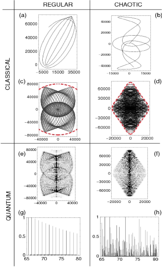
Figure 1: Illustration of the quantum-classical correspondence for the hydrogen atom in a magnetic field. The left column shows features when the dynamics of the classical system is regular, the right column when the dynamics is chaotic. (a)-(d) shows classical trajectories for the electron. (e)-(f) displays wavefunctions obtained from quantum computations for identical dynamical regimes [(e) as in (c), (f) as in (d)]. (g)-(h) gives an experimentally observable quantity (here obtained from quantum computations) by keeping again the dynamical regimes identical as above. See text (Sec. 3.3.2) for more details.

We will illustrate how the semiclassical interpretation works in practice by resorting to a specific example, the hydrogen atom in a magnetic field. This system has been thoroughly investigated both theoretically and experimentally and the semiclassical approximation is known to hold. Moreover from a de Broglie-Bohm standpoint, Bohmian trajectories for this system have been recently obtained (Matzkin 2006). Since an illustration involving the relation between spectral eigenvalue statistics and average classical properties would necessarily be very technical, we shall limit our examples to some global qualitative aspects and the rôle of the shortest classical periodic orbits, illustrated in Figs. 1 to 3.

The hydrogen atom in a uniform magnetic field $B$ is an effective nonseparable problem in two dimensions (due to cylindrical symmetry; for details the interested reader is referred to the review paper by Friedrich and Wintgen (1989)). The electron is subjected to the competing attractive Coulomb and magnetic fields. The dynamics of the classical system does not depend separately on the electron’s energy $E$ and the field strength $B,$ but on the scaled energy defined by the ratio $\epsilon=EB^{-2/3}$ (this property is due to a scaling invariance). When $\epsilon\rightarrow-\infty$ (in practice for $\epsilon\lesssim-0.7$) the Coulomb field dominates and the dynamics is regular (near-integrable regime). As the relative strength of the magnetic field increases, the classical dynamics turns progressively chaotic: a mixed phase-space situation holds for $-0.7\lesssim\epsilon\lesssim-0.2$ and for $\epsilon\gtrsim-0.15$ the phase space is fully chaotic (Poincaré surfaces of section are given in Friedrich and Wintgen (1989)). The scaling property also holds for the quantum problem, and one can therefore compute wavefunctions corresponding to a fixed value of $\epsilon.$

Fig. 1 encapsulates the nature of the quantum-classical correspondence for semiclassical systems. (a)-(d) show trajectories of the electron for the classical hydrogen in a magnetic field problem. $\varrho$ is the horizontal axis, $z$ the vertical axis (the magnetic field is in the $+z$ direction). The nucleus is fixed at $\varrho=0$, $z=0$. The scale is given in atomic units ($5.3\times 10^{-11}$ m), so that the trajectory spans a rather large distance for a microsystem (the electron goes as far as 0.01 mm from the nucleus). In (a)-(b), the electron is launched from the nucleus and evolves for a short time along the trajectory. The initial conditions are the same in (a) and (b), but the dynamical regime differs: (a) shows the trajectory when the dynamics of the classical system is regular ($\epsilon=-1$), and (b) when the dynamics is chaotic ($\epsilon=-0.15$). In (c) [resp. (d)] the trajectory shown in (a) [resp. (b)] evolves for a long time; in each case we have also plotted the symmetric trajectory (e.g. (c) shows (a) and the trajectory symmetric to (a) starting downward). The dashed line indicates the bounds of the region accessible to the electron at the given energy. When the dynamics is regular the trajectory evolves in a regular manner and occupies only a part of the accessible region in configuration space (this is due to the fact that in phase-space the trajectory is confined to a torus). When the dynamics is chaotic [(d)] the trajectory evolves disorderly and occupies ergodically all of the available region. (e)-(h) display features for the quantum hydrogen in a magnetic field problem. In (e) we have shown the density-plot of a wavefunction for the same dynamical regime (identical value of $\epsilon$) as the trajectory shown in (c) (the wavefunction was obtained by solving numerically the Schrödinger equation). The resemblance with (c) is explained semiclassically from the quantization of the torus explored by the classical trajectory. The wavefunction has a regular aspect (for example in the organization of the nodes). (d) gives the plot of the wavefunction when the corresponding classical system is in the chaotic regime as in (d). The wavefunction has a disordered aspect when compared to (e), and has an overall shape quite similar to the shape formed by letting a classical trajectory evolve as in (d). Finally, (g) and (h) show an experimentally observable quantity, the photoabsorption spectrum, that gives a rough idea of how the energy levels are distributed (the horizontal axis gives the energy of the level in terms of a number $\nu$ with $E=-1/2\nu^{2}$). Regular dynamics gives a photoabsorption spectrum with a regular aspect, characterized by evenly spaced lines (again a consequence of torus quantization which guarantees the existence of ’good’ quantum numbers). When the corresponding classical dynamics is chaotic, the spectrum [shown in (h)] has a complex aspect, reflecting the disappearance of an ordered structure in the underlying classical phase-space.

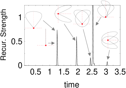
Figure 2: Recurrence spectrum of the hydrogen atom in a magnetic field obtained from quantum computations (the time is given in scaled units). The diagrams show the shape of the orbits closed at the nucleus of the corresponding (scaled) classical problem in the $(\varrho,z)$ plane ($B$ is along the vertical $z$ axis). The arrows indicate the orbit whose period matches the time of a given peak in the recurrence spectrum. Adapted from Matzkin (2006).

Fig. 2 shows a recurrence spectrum, giving the part of the initial wavefunction that returns to the nucleus as a function of time, the electron, initially near the nucleus, being excited at $t=0$. This spectrum results from a quantum computation but the same type of spectra has been observed experimentally (Main et al 1994). The peaks appear at times matching the period of the classical periodic orbits shown on the figure next to the peaks. The interpretative picture is the following: once the electron gets excited (e.g. by a laser), the wavefunction propagates in configuration space along the classical trajectories. Therefore the peaks in the recurrence spectrum indicate that the part of the wavefunction that returns to the nucleus does so by following the classical periodic orbits closed at the nucleus. Several orbits that have the same or nearly the same period can contribute to a given peak. In that case the phases $\phi_{k}$ of Eq. (8) which rule the interference between those orbits are crucial so that the semiclassical computations reproduce the exact height of the peak.

As a final illustration, Fig. 3 shows the localization of an energy eigenfunction on a periodic orbit of the classical problem. The left panel shows the wavefunction of an energy eigenstate when the corresponding classical dynamics is mixed (part of phase space is chaotic, part regular); the wavefunction was obtained by numerically solving the Schrödinger equation. The probability density is seen to occupy all of the available diamond-shaped region (as in Fig. 1(d)), but the striking feature is the very strong density concentrated on an spring-like shape. This shape is a periodic orbit of the classical system existing at the same energy. The periodic orbit, obtained by solving the classical equations of motion, is drawn on the right panel.

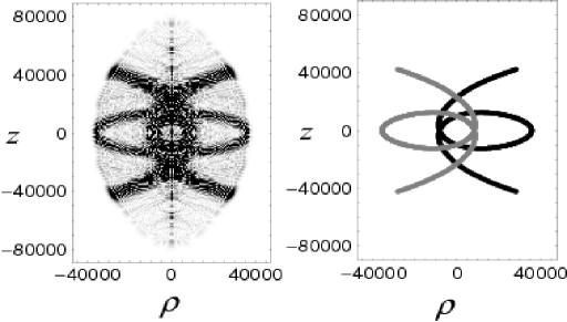
Figure 3: Left: Wavefunction of an excited energy eigenstate of the hydrogen atom in a magnetic field. Right: Periodic orbit of the corresponding classical system at the same energy (actually the periodic orbit [in black] is plotted along with its partner, symmetric by reflection on the $z$ axis [in gray]).

3.4 Status of the semiclassical interpretation

As we have introduced it, the semiclassical interpretation is an asymptotic approximation to the Feynman path integral. Whereas the exact path integral involves all the paths connecting two points in spacetime, the semiclassical approximation only takes into account the classical paths. It seems unwarranted to require more from the approximation than what is found in the exact expression, namely the propagation of a wave in configuration space by taking simultaneously all the available paths. No point particle can be attached to the path integral trajectories – it is actually an instance of a simultaneous sum over paths regarding the propagation of the wave. By itself the semiclassical interpretation cannnot and does not aim at explaining the emergence of classical mechanics from a quantum substrate. What does emerge are the structural properties (shape, stability) of the classical trajectories. In this sense, the small $\hbar$ condition (in relative terms) that defines the semiclassical regime appears as a necessary (but definitely not sufficient) ingredient in accounting for the classical domain. The semiclassical interpretation tells us that there are classical orbits in the wavefunction, but does not aim at unraveling what the wavefunction becomes in the classical world. Note that the same can be said regarding classical mechanics in the Hamilton-Jacobi formalism: this formalism contains the same classical theoretical entities that are employed in the semiclassical approximation. Obviously classical mechanics does not contain any traces of periodic wave propagation, but the wavefront of the classical action does propagate like a shock wave in configuration space (see Sec. 10-8 of Goldstein (1980)). As a theoretical entity the action is by itself a non referring epistemic term and it is only by making additional assumptions that the motion of an ensemble of trajectories can be extracted from the propagating wavefront of the action, recovering the ontology of classical mechanics in Newton’s form.

We point out notwithstanding that the semiclassical interpretation has also been considered as a theory in its own right, distinct from classical but also from quantum mechanics (Batterman 1993, 2002). Such an assessment has been made on the basis of the different nature of the explanations afforded by the semiclassical interpretation relative to the standard quantum theory: Batterman argues that emergent properties are characteristic of asymptotic theories, as these cannot be reduced to the fundamental theories that lack the conceptual resources necessary to the interpretation of asymptotic phenomena. Without necessarily endorsing this viewpoint, the semiclassical interpretation nevertheless attributes to the classical concepts it employs similar virtues. The fact that one ignores what the quantum-mechanical theoretical entities refer to explains why the putatively fundamental theory (quantum mechanics) is unable to account for the emergence of classical mechanics, and why in semiclassical physics the interpretative framework relies essentially on classical conceptual resources. Hence in semiclassical physics one speaks of the quantum properties as being ”determined” by the properties of the underlying classical system, or on the wavefunction ”depending” on the classical trajectories. It must be remembered however that stricto-sensu, the semiclassical interpretation only establishes an enlarged, precise and universal correspondence between the properties of quantum systems in the semiclassical approximation and those of their classical equivalents.

4. BOHMIAN TRAJECTORIES IN THE SEMICLASSICAL REGIME

4.1 From quantum to classical trajectories

As mentioned in Sec. 2, one of the main advantages of the de Broglie-Bohm interpretation is that BM allows to bridge the quantum and classical worlds, by way of a quantum point-like particle following a precise trajectory. Of course, trajectories in the quantum domain are generically nonclassical, due to the presence of the quantum potential. This quantum state dependent potential enters the equations for the Bohmian trajectories in Eq. (2); without this term Eq. (2) would become the classical Hamilton-Jacobi equation (9). The presence of the quantum potential term in Eq. (2) leads to highly nonclassical solutions even for intuitively simple systems. The best-known example is probably the particle in a box problem, which raised Einstein’s well-know criticism of the de Broglie-Bohm interpretation (a thorough discussion can be found in Sec. 6.5 of Holland 1993): classically a particle in a box would follow a to and fro motion, its constant velocity being reversed when the particle hits the boundary of the box. According to BM however there is no particle motion, because the quantum potential cancels the classical kinetic energy. The same behaviour arises for stationary wavefunctions like the energy eigenstates: for example the electron in a hydrogen atom is either at rest (if the azimuthal quantum number is 0) or it displays an asymmetric motion around the quantization axis. On the other hand the classical trajectories for that system (the familiar ellipses of planetary motion) need to fulfil the symmetry of the classical potential (just as the wavefunction does), which is broken by the quantum potential term.

Now having Bohmian trajectories in the quantum domain different from the trajectories in the classical domain is not necessarily a problem. The problem is that as the classical world is approached, there are no physical criteria that will unambiguously make the quantum potential vanish and lead to classical trajectories, irrespective of how the classical limit is defined. Different opinions to circumvent this important difficulty from a physical standpoint have been given (these arguments will be developed and discussed in Sec. 5). One possibility is that some quantum systems, or specific states thereof (such as the energy eigenstates) simply do not have a classical limit (Holland 1993); conversely some classical systems may not be obtained as limiting cases of an underlying quantum problem, entailing that BM and classical mechanics would have exclusive (albeit partially overlapping) domains of validity (Holland 1996, Cushing 2000). Another argument asserts that since closed quantum systems cannot be observed in principle (since they always interact with a measurement apparatus, an environment etc.), ’apparent’ trajectories (resulting from the measurement interaction) are bound to be different from the ’real’ ones (Bohm and Hiley 1993, Ch. 8). But if trajectories could be inferred without perturbing a quantum system, the ones predicted by BM would be found, not the classical ones (Bohm and Hiley 1985). More recently tentative proposals of recovering classical trajectories from Bohmian mechanics in simple systems by combining specific types of wavepackets and environmental decoherence arising from interactions with the environnement have been put forward (Appleby 1999b, Bowman 2005), although these treatments lack sufficient generality. In this context, the specificity of semiclassical systems follows from the fact that they are closed quantum systems that nevertheless display the manifestations of classical trajectories. It is thus instructive to examine the behaviour of Bohmian trajectories in semiclassical systems.

4.2 Bohmian trajectories and semiclassical wave-propagation

It is straightforward to make the case that in semiclassical systems Bohmian trajectories are highly nonclassical, as in any quantum system. Indeed in the de Broglie-Bohm interpretation, the velocity field given by Eq. (4) is proportional to the quantum mechanical probability density current $j(x,t)=\hbar\psi^{\ast}(x,t)\overleftrightarrow{\nabla}\psi(x,t)/2mi$ through $j=\rho^{2}v$ (recall $v(x,t)$ is the velocity of the Bohmian particle). Since frome Eq. (8) an evolving wavefunction takes the form

$$\psi(x,t)=\sum_{k}A_{k}(x,x_{0},t)\exp i(R_{k}(x,x_{0},t)/\hbar-\phi_{k}),$$ (13)

where $A_{k}$ includes the determinant of the propagator and quantities relative to the initial wavefunction, the probability current $j(x,t)$ at some point $x$ will be given by a double sum containing interference terms: the net probability density current arises from the interference of several classical trajectories taken simultaneously by the wave, as required by the path integral formulation. Therefore except in the exceptional case in which there is a single classical trajectory (that the probability current must therefore follow), the net probability density guiding the Bohmian particle will not flow along one of the classical trajectories that act as backbones of the wavefunction in the semiclassical regime. The particle in a box case gives a particularly simple illustration. At a fixed energy, there are only 2 classical trajectories passing through a given point, one in each direction, so that the net probability flow is 0, translating in BM as no motion for the particle.

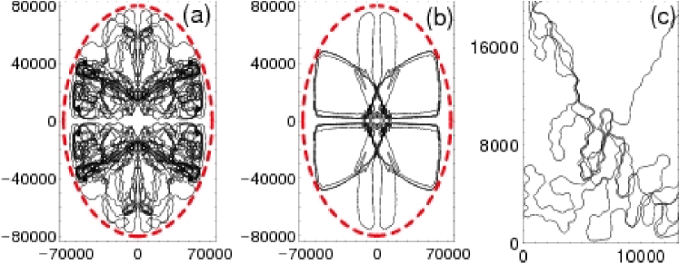
Figure 4: Bohmian trajectories for the hydrogen in a magnetic field problem in the regular regime of Fig. 1 (classical regular trajectories, ordered quantum properties). (a) and (b) each contain a single trajectory in the $\varrho>0$, $z>0$ quadrant and 3 symmetric replicates of this trajectory in the other quadrants (see text). The initial position of the Bohmian electron is the same in (a) and (b), but the initial quantum state is different. (c) shows a zoom of (b) in the region near the nucleus (for the positive quadrant only). The dashed lines indicate the bounds of the classically accessible region, as in Fig. 1.

For the hydrogen atom in a magnetic field problem examined in Sec. 3, de Broglie-Bohm trajectories can be computed and compared to the classical ones (Matzkin 2006). Typical Bohmian trajectories for the electron are shown in Figs. 4 and 5, for the dynamics in the regimes shown in Fig. 1. Fig. 4 shows trajectories corresponding to the regular column in Fig. 1 ($\epsilon=-1$ corresponding to classical regular trajectories and quantum properties having a regular aspect). The sole difference between Fig. 4(a) and (b) concerns the choice of the initial wavefunction (which contains more eigenstates in case (a)). It is important to stress that a Bohmian trajectory cannot cross either the $\varrho$ or $z$ axis. Figs. 4(a) and (b) contain each a Bohmian trajectory in the $\varrho>0$, $z>0$ quadrant and three symmetric copies of this trajectory in the remaining quadrants (in agreement with the symmetry of the statistical distribution). The trajectory in Fig. 4(a) has a chaotic aspect and occupies most of configuration space, whereas the trajectory in Fig. 4(b) has a more regular aspect, as the Bohmian particle retraces several times a similar figure. However when this trajectory is zoomed in the region near the nucleus (Fig 4(c); we only show the ’original’ trajectory in the positive quadrant), the regular aspect is not evident. We therefore see that the correspondence between the classical dynamical regime and quantum properties encapsulated in Fig. 1 is not obeyed by BB trajectories. The converse is also true: Fig. 5 shows a Bohmian trajectory (and its 3 symmetric replicates) in the chaotic dynamical regime of the right column of Fig. 1 (classically chaotic trajectories and disordered quantum properties). The Bohmian trajectory is visibly regular, in the sense that the particle retraces the same regions of space in a similar fashion as can be seen in the zoom, Fig. 5(b), and occupies only a small part of the region of configuration space available to the particle.

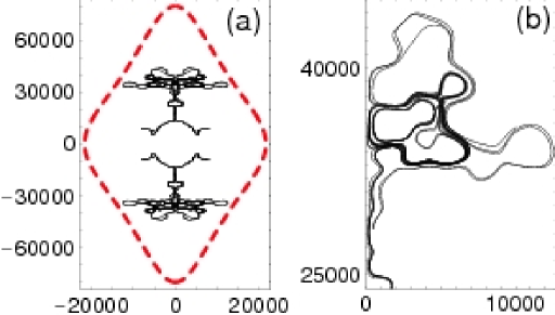
Figure 5: Same as Fig. 4 but in the chaotic regime of Fig. 1 (classical chaotic trajectories, disordered quantum properties). (a) shows a Bohmian trajectory in the positive quadrant and its 3 replicates, (b) zooms in a specific region.

Another difference in the behaviour of de Broglie-Bohm trajectories with regard to the quantum-classical correspondence for semiclassical systems can be seen in the energy eigenstates. The eigenstates are organized and sometimes localized along the periodic orbits of  the classical hydrogen in a magnetic field problem as seen in Fig. 3, but a Bohmian particle in an energy eigenstate has no motion in the $(\varrho,z)$ plane (it has no motion at all if $m=0,$ or orbits around the $z$ axis so that the trajectory remains still in the $(\varrho,z)$ plane if $m\neq 0$). We also note as another consequence of the nonclassical nature of the BB trajectories that the periodic recurrences of the type shown in Fig. 2, which appear at times matching the periods of return of classical closed orbits (and their repetitions), cannot be produced by a an individual Bohmian trajectory. Indeed Bohmian trajectories do not possess the classical periodicities visible in the peaks, and an ensemble of different Bohmian trajectories compatible with a given statistical distribution is necessary to account for the recurrences (Matzkin 2006). This is a straightforward consequence stemming from the fact that a Bohmian particle moves along the streamlines of the probability flow. Then the evolution of the wavefunction between the initial and the recurrence times can only be obtained if the complete ensemble of streamlines is taken into account (Holland 2005).

4.3 Quantum chaos and the quantum-classical correspondence

We have given examples of de Broglie-Bohm trajectories for the hydrogen atom in a magnetic field problem and seen that their features are unrelated to the properties of the underlying classical system and therefore do not fit in the quantum-classical correspondence scheme arising from the semiclassical interpretation. This is of course a general statement: analogue results were obtained for square and circular billiards, which are classically integrable systems, but where Bohmian trajectories were found to be either regular or chaotic, depending on the choice of the initial wavefunction (the initial state that also gives the initial statistical distribution) (Alcantara-Bonfim et al 1998). In right triangular billiards chaotic or regular Bohmian trajectories were found for the same initial distribution but different initial position of the particle (de Sales and Florencio 2003). In one of the earliest studies of the Bohmian approach to quantum chaos (Parmenter and Valentine 1995), a two dimensional uncoupled anisotropic harmonic oscillator (a separable system having a deceptively simple regular classical dynamics) was shown to display chaotic Bohmian trajectories (see also Efthymiopoulos and Contopoulos 2006).

The chaotic nature of Bohmian trajectories is due to the state-dependent quantum potential, given by Eq. (5). In particular when $\rho(x,t)$ vanishes, the quantum potential becomes singular. This happens at the nodes of the wavefunction. Employing the hydrodynamic analogy (the probability density flow carries the BB trajectories), the nodes correspond to vortices of the probability fluid. It has recently been confirmed (Wisniacki and Pujals 2005) that the vortices are at the origin of the generic chaotic behavior of Bohmian trajectories; these authors obtained chaotic trajectories even in an isotropic harmonic oscillator, the ’most regular’ classical integrable system. Conversely since as we have just mentioned a Bohmian particle has no motion in an eigenstate, it is always possible to obtain a regular Bohmian trajectory (even for a disordered quantum system corresponding to classically chaotic dynamics) by taking an initial distribution composed of a 2 or 3 eigenstates with a very strong weight for one of these states.

Thus, from the perspective developed in this paper, it is clear that Bohmian mechanics spoils the quantum-classical correspondence that arises in the semiclassical regime, in the sense that de Broglie-Bohm trajectories can be chaotic or regular irrespective of the dynamical characteristics of the corresponding classical system which are in correspondence with observable quantum properties. As we have emphasized above, the energy eigenstates in quantum semiclassical systems are organized around the phase-space structures of the corresponding classical system (Fig. 2). The distribution of the energy levels is also directly dependent on the underlying classical dynamics in two ways: a universal relation valid for any system, depending on the mean properties of the periodic orbits, and a system specific behaviour, depending on individual periodic orbits. In the de Broglie Bohm approach, the trajectories are entirely determined by the precise form of the quantum-mechanical wavefunction: there is no manner in which the topology of the trajectories can account for the structural aspects of the wavefunction. This is why quantum chaos in Bohmian terms and quantum chaos understood in the semiclassical sense are radically divergent. The former strives to define chaos exactly as in classical mechanics, by examining the properties of quantum trajectories; but Bohmian trajectories will necessarily remain unrelated to the properties of the corresponding classical system, and will be unable to explain the manifestations of chaotic classical trajectories in quantum systems. On the contrary, quantum chaos in the semiclassical sense accounts for purely quantum mechanical features by linking them to the dynamical properties of the corresponding classical system, in particular to its chaoticity; but as we have mentioned above, the semiclassical interpretation has no more ontological ambition than what is found in the path integral formulation of quantum mechanics.

5. CONSTRAINTS ON THE EMPIRICAL ACCEPTABILITY AND REALITY OF BOHMIAN TRAJECTORIES IN SEMICLASSICAL SYSTEMS

From within a purely internal quantum approach governed by the Schrödinger equation, semiclassical systems have a peculiar property: the dynamics of these quantum systems depends on the trajectories of the corresponding classical system. This ’peculiar property’ arises naturally in the path integral formulation. On the other hand, we have seen above that the de Broglie-Bohm interpretation appears to contradict the enlarged version of the quantum-classical correspondence stemming from the semiclassical interpretation. From the standpoint of the benefits that should emerge from adopting Bohmian mechanics (see Sec. 2), this may appear as unexpected. Indeed, if BM is unable to account for the presence of classical trajectories in semiclassical quantum systems, how will the interpretation explain the emergence of macroscopic classical trajectories? Taking the de Broglie-Bohm interpretation as a realist construal of quantum phenomena, what is implied when asserting with BM that the trajectories of the particles are highly nonclassical in reality although the shape of the classical trajectories is directly visible in the wavefunction? These questions touch upon issues that have been examined in more general contexts by supporters and critics of the interpretation, but these issues take in semiclassical systems a particularly acute form. We review the type of answers that have been given and examine their implications regarding a de Broglie-Bohm account of semiclassical systems.

A first argument involves a reassessment of the relation between quantum and classical mechanics considered as fundamental physical theories. We have seen above that a strong motivation for embracing the de Broglie Bohm interpretation is that BM allows to fill the gap between the quantum and the classical domains. BM would thus provide ”an attractive understanding of the classical limit” (Callender and Weingard 1997). Given that as far as the dynamics is concerned Bohmian trajectories in closed systems are not classical, this motivation is reassessed by putting the stress on the ontological continuity while questioning the necessity that classical mechanics needs to emerge from the quantum substrate. This is why Holland (1996) suggests that quantum and classical mechanics should be regarded as two different theories having a partial overlap: the latter should not be expected to emerge from the former. This move allows Holland to conclude that the fact that ”classical dynamics is not generally a special case [of the de Broglie Bohm approach] has then no implications for the validity of the interpretation” (p. 109). Hence the dynamical mismatch between BB and classical trajectories cannot constitute an objection, each theory having its own domain of validity. Applying this argument to semiclassical systems is however not straightforward: these systems are characterized by the manifestations of classical trajectories, implying for the least a minimal partial overlap that is not reflected in the dynamics of the Bohmian particle. To stand by Holland’s conclusion, one would need to assume that semiclassical systems constitute an instance of non-overlap for the dynamics of the particle (since the Bohmian trajectories are nonclassical) despite having the quantum wavefunction organized according to the underlying classical phase-space, and thus in correspondence with the motion of the particle in the corresponding classical system, thereby displaying a type of overlap on a different level.

Arguments of the same kind have been made on quantum chaos, where the non-overlap is now made between the aspect of the wavefunction and the dynamics of the Bohmian particle. As concisely put by Cushing (2000) ”BM has certain conceptual and technical resources (not available in standard QM) that allow it to address, and arguably to resolve, two long-standing and difficult issues in quantum theory (i.e., the classical limit and quantum chaos)”. In the de Broglie-Bohm theory, these specific conceptual resources – and therefore the issues of quantum chaos and the classical limit – involve the particle dynamics, not the wave. Commenting their findings on the chaotic Bohmian trajectories obtained in a classically integrable system, Parmenter and Valentine (1995) can thus state that ”there is no contradiction between the fact that the wave-function associated with a quantum mechanical state is not chaotic, while at the same time a causal trajectory associated with the state is chaotic”. A contradiction can indeed be avoided but at the expense of an account containing at least three levels of explanation: the Bohmian dynamics level, determined by the wavefunction, which in turn is determined, for semiclassical systems, by the underlying classical phase-space. Hence regular classical dynamics is reflected in a regular quantum wavefunction but not in the chaotic Bohmian trajectories that are the ones followed by the particle ’in reality’. Therefore the necessary non-overlap between the wave aspect and the dynamics of the Bohmian particle yields in semiclassical systems another instance of the dynamical mismatch between BB and classical trajectories, only the latter being reflected in the aspect of the wavefunction. The same type of explanation must be considered to explain the localization of the energy eigenstates on the classical periodic orbits as in Fig. 3: the wavefunction is organized around the classical periodic orbits, the probability density of the wave reflecting precisely the classical density distribution (i.e., the classical amplitude of a pencil of classical trajectories). In the BB approach, this means that the statistical distribution of Bohmian particles depends on the properties of the classical periodic orbits present in the wavefunction; but the motion of the Bohmian particles will be unrelated to the classical motion. Again, it is consistent in BB terms to dismiss any requirement of overlap between the dynamics of the particle and the aspect of the wavefunction, but in semiclassical systems this move implies a non-overlap with the classical trajectories of the particle that actually determine the shape of the wavefunction.

Although the non-overlap type of explanations may have an overdone flavour when applied to semiclassical systems, it seems impossible to avoid them if the de Broglie-Bohm interpretation is taken as a realist account of the quantum mechanics of semiclassical systems. The reason is the incompatibility between the hydrodynamic picture underlying the motion of the BB particle along a single path connecting two spacetime points on the one hand, and the wave picture where the wave takes simultaneously all the multiple interfering paths between the two points on the other. In the hydrodynamic picture the motion of the particle depends entirely on the local properties of the probability density flow. In the wave picture the paths actually construct the wavefunction. Hence if semiclassical wavefunctions are built from classical paths, a Bohmian trajectory will only be sensitive to the necessarily nonclassical flow. It is noteworthy that proponents of the de Broglie Bohm interpretation tend to dismiss the path integral approach as a mathematical tool without any substantial physical implication (e.g. Sec. 6.9 of Holland (1993)). The semiclassical systems discussed in this work contradict this assertion since the classical dynamics is directly reflected in the wavefunction, and observable quantities such as recurrence spectra display in an unequivocal way the interfering paths (see the example given in Fig. 2). 

A different argument of epistemological nature has often been put forward to explain the irrelevance of the non-classical behaviour of Bohmian trajectories to the quantum-classical transition problem. Since BB trajectories in closed system are unobservable in principle (they are hidden), no observable consequences can arise from their non-classicality. When observed, the quantum system will be interacting with an environment (such as a measurement apparatus). The apparent Bohmian trajectory of the open interacting system is the one that should be compared to the classical trajectory, not the real trajectory of the isolated system. Hence the motion along an individual BB trajectory of a closed system has no bearing on the empirical acceptability of the theory, provided the statistical predictions of quantum mechanics are recovered (Appleby 1999a). In a general context, Fine (1996) remarked that this type of argument employs the same positivist lines of defense that are generally found in vindication of the Copenhagen interpretation, namely that what matters is the predictive agreement with experiments and that it is impossible in principle to observe isolated, noninteracting systems or trajectories. But departing from standard quantum mechanics, which states that describing an isolated system has no meaning, BM proposes a full description, in terms of waves and particles trajectories, of the reality of an individual isolated system. The specific difficulty arising for semiclassical systems is that classical trajectories are present in the wavefunction of the closed system. Since Bohmian mechanics regards the wavefunction as a real field, the retreat behind the shield of the sole empirical acceptability may appear as insufficient: in view of the epistemological advantages associated with the de Broglie-Bohm approach recalled in Sec. 2.2 (Cushing 1994), one would expect a dynamical explanation for the presence of the classical trajectories in the wavefunction (the statistical distribution) while individual trajectories followed by the Bohmian particle are all nonclassical. Furthermore, even if one accepts that classical trajectories arise dynamically from environmental interactions, the fact is that the noninteracting semiclassical systems display several observable manifestations of the classical trajectories.

The question then becomes under which conditions it is plausible to assume that the real (nonclassical) Bohmian trajectory of the closed semiclassical system can be markedly different from the (classical) apparent trajectory of the measured interacting system even though the pilot-wave of the closed system is itself built on these classical trajectories, whose manifestations are experimentally observed. The dynamical mismatch induces a tension between the supposedly real dynamics of the particles (following de Broglie-Bohm trajectories), the statistical distribution of the particles (determined by the underlying classical properties) and the classical trajectories (observed by means of a physical interaction). In this respect, it may be noted that the justification of the ”special assumption” (Holland 1993, p. 99) by which the guiding field $\psi$ gives at the same time the statistical distribution of the particles $\rho^{2}$ has always been a delicate point in the de Broglie-Bohm approach. We are not questioning the possibility that specific auxiliary assumptions can be added to the ’special assumption’, so that in semiclassical systems the statistical distribution $\rho^{2}$ is made to depend on the classical dynamics, but not the motion of the Bohmian particle, except when interacting with a specific environment, inducing the oberved classical trajectories. We should however consider such auxiliaries relative to the motivational advantages associated with the interpretation, viz. the extension of realism to the domain of quantum phenomena and the unification of classical and quantum mechanics. On both of these points, semiclassical systems bring specific constraints that must be met by Bohmian mechanics to ensure a credible account of the dynamical properties of these systems. Regarding the first point we will only mention here the realist demand for epistemic constraints on the auxiliary assumptions so as to avoid ad-hoc explanations and the ensuing underdetermination dilemmas, given that the real dynamical behaviour of a quantum system cannot be at the same time chaotic and regular. As for the second point our account of the physics of semiclassical systems suggests that classical mechanics appears in the quantum world by structuring the wavefunctions, rather than by orchestrating the streamlines of the probability flow. This statement must actually hold to explain the correspondence between quantum and classical systems illustrated in Fig. 1. Since semiclassical systems constitute a bridge between the quantum and the classical worlds, the status of Bohmian trajectories in such systems hinges on a better understanding of the relations between the hydrodynamic picture and the path integral formulation of quantum phenomena, and of a possibly elusive unification of both formulations.

6. CONCLUDING REMARKS

Pauli was among the first to criticize both de Broglie’s first proposal of the pilot-wave (at the 1927 Solvay conference) as well as Bohm’s rediscovery of it some 25 years later. In his contribution to de Broglie’s 60th birthday volume, Pauli (1952) dismissed the de Broglie-Bohm approach as ”artificial metaphysics” because the BB approach breaks the correspondence between classical mechanics and standard quantum mechanics regarding the symmetric treatment of canonically conjugate variables. Indeed, in quantum mechanics a Fourier transform links the representation of the wavefunction in terms of one variable (e.g. the position) to the representation in terms of its canonical conjugate (the momentum). In the BB approach the position representation is the only meaningful one; the momentum of the Bohmian particle is given by the guidance equation, not by a Fourier transform. Pauli’s criticism is certainly not accidental: although less well-known Pauli was the first to obtain the correct form of the semiclassical propagator from the Feynman path integral (Choquard and Steiner 1996). In the semiclassical approximation the Fourier transform gives the purely classical relation between the two action functions, one expressed in terms of one variable (the position), the other in terms of its canonical conjugate (the classical momentum of the particle).

It would appear that a formal objection favouring a correspondence relation between theoretical entities in two different physical theories (quantum and classical mechanics) challenges the ontological continuity postulated by Bohmian mechanics, which is grounded on a particle guided by the current density of the wave. However, one of the conclusions of this work is that this objection is not purely formal, because semiclassical systems do exist in nature. We have seen that the consequences of this quantum-classical correspondence are visible in semiclassical systems through the manifestations of classical trajectories on the quantum observables. The dynamics predicted in the de Broglie-Bohm approach, assumed to represent the real motion of a quantum particle, conflicts with this correspondence. Interestingly, the ontological continuity posited in the de Broglie-Bohm interpretation as well as the quantum-classical correspondence that transpires in semiclassical systems both go one way, from the classical down to the quantum world (in terms of classical-like particles pursuing nonclassical trajectories in the first case, in terms of nonclassical waves moving on classical trajectories in the latter). Yet in both cases, the missing piece of the puzzle can only be put into place by finding the proper upward way.

References

- (1) Alcantara-Bonfim, O. F. de, Florencio, J. and Sa Barreto, F. C. (1998). Chaotic dynamics in billiards using Bohm’s quantum dynamics. Physical Review E, 58, R2693-R2696.
- (2) Appleby, D. M. (1999a). Generic Bohmian trajectories of an isolated particle. Foundations of Physics, 29, 1863-1883.
- (3) Appleby, D. M. (1999b). Bohmian Trajectories Post-Decoherence. Foundations of Physics, 29, 1885-1916.
- (4) Arnold, V. I. (1989). Mathematical Methods of Classical Mechanics, New York: Springer.
- (5) Batterman, R.W., (1993). Quantum chaos and semiclassical mechanics, in PSA: Proceedings of the Biennial Meeting of the Philosophy of Science Association 1992, volume 2, pages 50-65.
- (6) Batterman, R.W., (2002). The Devil in the Details – Asymptotic Reasoning in Explanation, Reduction, and Emergence, Oxford:Oxford University Press.
- (7) Berry, M. V. (1991). Some quantum-to-classical asymptotics, in Les Houches Lecture Series LII, eds. Giannoni M., Voros A. and Zinn-Justin J, Amsterdam:North-Holland, 251-304.
- (8) Bohm, D. (1952). A suggested interpretation of the quantum theory in terms of ”hidden” variables. Physical Review, 85, 166-193
- (9) Bohm, D. and Hiley, B. J. (1985). Unbroken quantum realism from microscopic to macroscopic levels. Physical Review Letters, 55, 2511-2514.
- (10) Bowman G. (2005). On the Classical Limit in Bohm’s Theory. Foundations of Physics 35 (2005), 605-625
- (11) Bohm, D. and Hiley, B. J. (1993). The Undivided Universe: an ontological interpretation of quantum theory, London: Routledge.
- (12) Brack M. and Bhaduri R. K. (2003), Semiclassical Physics, Reading(USA):Addison-Wesley.
- (13) Broglie, L. de (1927). La mécanique ondulatoire et la structure atomique de la matière et du rayonnement. Journal de Physique VI, 8, 225-241.
- (14) Callender, C. and Weingard, R. (1997). Trouble in paradise? Problems for Bohm’s theory. The Monist, 80, 24-43.
- (15) Choquard P. and Steiner, F. (1996). The Story of Van Vleck s and Morette-Van Hove s Determinants. Helvetica Physica Acta 69, 636-654.
- (16) Cushing, J. T. (1994). Quantum mechanics: historical contingency and the Copenhagen hegemony, Chicago: Chicago University Press.
- (17) Cushing, J. T. (1996). The causal quantum theory program, in cushing et al. (1996), p. 1-19.
- (18) Cushing, J. T. (2000). Bohmian insights into quantum chaos. Philosophy of Science, 67, S430-S445.
- (19) Cushing, J. T., Fine, A.. and Goldstein, S., eds. (1996) Bohmian mechanics and quantum theory: an appraisal. Boston Studies in the Philosophy of Science vol. 184, Kluwer: Dordrecht.
- (20) Devitt M.(2002). Underdetermination and Realism. Nous, Supp. Philosophical Issues 12, 26-50.
- (21) Dürr D, Goldstein S and Zanghi N. (1996). Bohmian mechanics as the foundation of quantum mechanics, in Cushing et al. (1996), p 21-44
- (22) Efthymiopoulos C. and Contopoulos G. (2006). Chaos in Bohmian quantum mechanics. Journal of Physics A: Mathematical and General, 39, 8563-8563.
- (23) Fine, A. (1996). On the interpretation of Bohmian mechanics. In Cushing et al. (1996), p. 231-250
- (24) Friedrich H. and Wintgen D. (1989). The hydrogen atom in a uniform magnetic field An example of chaos. Physics Reports 183, 37-79.
- (25) Goldstein, H. (1980), Classical Mechanics, Addison-Wesley, Reading (USA).
- (26) Grosche C. and Steiner F. (1998), Handbook of Feynman Path Integrals, Springer Tracts in Modern Physics 145.
- (27) Gutzwiller, M. C. (1990). Chaos in classical and quantum mechanics, Berlin: Springer.
- (28) Haake, F. (2001). Quantum signatures of chaos, Berlin: Springer.
- (29) Holland P.R. (1993), The Quantum Theory of Motion, Cambridge Univ. Press, Cambridge.
- (30) Holland P.R. (1996). Is quantum mechanics universal, in Cushing et al. (96), p 99-110.
- (31) Holland, P. R. (2005). Computing the wavefunction from trajectories: particle and wave pictures in quantum mechanics and their relation. Annals of Physics 315, 505-531.
- (32) Home, D. (1997). Conceptual foundations of quantum physics: an overview from modern perspectives, London: Plenum.
- (33) Main J., Wiebusch G., Welge K. H., Shaw J. and Delos J. B. (1994). Recurrence spectroscopy: Observation and interpretation of large-scale structure in the absorption spectra of atoms in magnetic fields. Physical Review A 49, 847-868.
- (34) Matzkin, A. (2006). Can Bohmian trajectories account for quantum recurrences having classical periodicities?. Physics Letters A 361, 294-300, 2007 [ArXiv.org Eprint quant-ph/0607095].
- (35) Matzkin, A. and Monteiro, T. S. (2004). Spectral rigidity in scatterer-perturbed systems: the case of nonhydrogenic atoms in fields. Journal of Physics A: Mathematical and General, 37, L225.
- (36) Maudlin, T. (1995). Why Bohm’s theory solves the measurement problem. Philosophy of Science, 62, 479-483.
- (37) Norris, C. (1999). Quantum theory and the flight from realism: philosophical responses to quantum mechanics, London: Routledge.
- (38) Parmenter, R. H. and Valentine, R. W. (1995). Deterministic chaos and the causal interpretation of quantum mechanics. Physics Letters A 201, 1-8.
- (39) Pauli, W. (1952). Remarques sur le problème des paramètres cachés dans la mécanique quantique et sur le théorie de l’onde pilote, in André George (Ed.), Louis de Broglie Physicien et Penseur, Paris: Albin Michel, p. 33-42.
- (40) Putnam, H. (1965). A Philosopher looks at quantum mechanics. Reprinted in Putnam, H. (1975), Philosophical papers, Vol. 1, Cambridge: Camnbridge University Press, p. 130-158.
- (41) Putnam, H. (2005). A Philosopher looks at quantum mechanics (again). British Journal for the Philosophy of Science 56, 615-634.
- (42) Sales J. A. de, and Florencio, J. (2003). Quantum chaotic trajectories in integrable right triangular billiards. Physical Review E 67 016216.
- (43) Wisniacki, D. A. and Pujals, E. R. (2005). Motion of vortices implies chaos in Bohmian mechanics. Europhysics Letters 71, 159.
- (44) Zeh, H. D. (1999). Why Bohm’s quantum theory. Foundations of Physics Letters, 12, 197-200.