Single-bit Feedback and Quantum Dynamical Decoupling

Abstract

Synthesizing an effective identity evolution in a target system subjected to unwanted unitary or non-unitary dynamics is a fundamental task for both quantum control and quantum information processing applications. Here, we investigate how single-bit, discrete-time feedback capabilities may be exploited to enact or to enhance quantum procedures for effectively suppressing unwanted dynamics in a finite-dimensional open quantum system. An explicit characterization of the joint unitary propagators correctable by a single-bit feedback strategy for arbitrary evolution time is obtained. For a two-dimensional target system, we show how by appropriately combining quantum feedback with dynamical decoupling methods, concatenated feedback-decoupling schemes may be built, which can operate under relaxed control assumptions and can outperform purely closed-loop and open-loop protocols.

I Introduction

The role of real-time measurement and information feedback in designing control strategies is well recognized for a wide range of applications in classical control theory Doyle et al. (1992). Feedback in the quantum domain, however, unavoidably involves additional challenges due to the intrinsically probabilistic Sakurai (1994); Holevo (2001) and, typically, destructive character of the quantum measurement process von Neumann (1955) – leading to a host of delicate issues and added difficulties for many tasks of interest to the emerging field of quantum control. As a result, real-time quantum feedback is nowadays actively investigated at both the theoretical and experimental level. In particular, continuous-time feedback strategies, based on indirect weak measurements, have been originally proposed for cavity QED systems Wiseman and Milburn (1993); Wiseman (1994), and have recently begun to be experimentally accessible Geremia et al. (2004); Smith and Orozco (2004). From a control-theoretic standpoint, a general analysis of strategies based on average measurements on quantum ensembles and feedback has been considered in Altafini (2005). Suggestive applications of continuous measurements and feedback in the context of quantum error correction have also been investigated Ahn et al. (2003).

Our focus in this work is to begin exploring possible uses and advantages of discrete-time quantum feedback, based on strong projective measurements, in connection with a fundamental quantum control task: engineering a desired unitary operation on a target system, which may be generally interacting with an uncontrollable quantum environment. Thus, given a set of available control operations, the goal is to design a protocol capable to enforce a desired net evolution on the system at a given final time, irrespective of the system’s initial state. This problem, unlike the simpler case of state preparation, forces in general the introduction of indirect measurements on a suitable ancillary system. The first step in this direction is to employ the minimum physical amount of information we can gather, a single bit. In particular, in what follows, we aim to construct and test protocols for engineering the simplest unitary operation (the identity or no-op gate Nielsen and Chuang (2002)) by using, along or in conjunction with additional control schemes, a feedback loop built from basic, arbitrarily fast and accurate control operations.

The analysis and techniques presented here exploit and extend ideas close to those introduced in a number of earlier works. In particular, our ancillary qubit system may be seen as a concrete instance of a quantum controller Lloyd (2000) or, more generally, a universal quantum interface Lloyd and Viola (2001); Lloyd et al. (2004). Control schemes exploiting auxiliary quantum probe systems and measurement capabilities have also been recently discussed in Mandilara and Clark (2005); Romano and D’Alessandro (2005). However, while the main emphasis of the above-mentioned literature is on establishing general existential results on quantum accessibility and controllability, our interest here is on providing constructive, synthesis results instead.

Two main families of protocols emerge: on one hand, feedback-enacted decoupling protocols – which, in the infinitesimal time limit, directly relate to feedback implementations of quantum dynamical symmetrization procedures Viola et al. (1999); Zanardi (1999) and, when appropriate conditions are met, allow to relax the fast control limit of open-loop schemes; on the other hand, feedback-concatenated decoupling protocols – whereby the output of a primary open-loop dynamical decoupling (DD) protocol serves as input to an outer feedback block, or viceversa. Interestingly, the analysis of the feedback-enacted procedures may be also regarded as stemming from the communication-oriented approach of Gregoratti and Werner (2003, 2004), or as a particular instance of a quantum error-correction procedure Nielsen et al. (1998). In a similar spirit, an interesting discussion on the ensuing trade-off between information gain and disturbance for different measurement strategies in a single-qubit setting can be found in Brańczyk et al. (2006). From a technical point of view, our main results further demonstrate the usefulness of linear algebraic methods for finite-dimensional quantum control settings, along the lines introduced in Ticozzi and Ferrante (2004).

The content of the paper is organized as follows. Following a presentation of the general control-theoretic setting in Section II, we develop our main theoretical analysis and results for a generic finite-dimensional target system in Section III. By restricting to the simple yet paradigmatic case of arbitrary state stabilization for a single qubit, in Section IV we describe various concatenated feedback-decoupling protocols built, in particular, from both maximal and selective DD schemes Viola et al. (1999); Haeberlen (1976). The performance of different schemes in the non-ideal limit of finite control time scales is numerically investigated and compared in Section V. A discussion and concluding remarks follow.

II System and control settings

We will consider a finite-dimensional quantum system $\mathcal{S}$, coupled in general to an uncontrollable, possibly unknown quantum environment $\mathcal{E}$. Let $\mathcal{H}_{\mathcal{S}}$ and $\mathcal{H}_{\mathcal{E}}$ denote the system and the environment Hilbert spaces, with dim($\mathcal{H}_{\mathcal{A}}$)= $d_{\mathcal{S}}$, dim($\mathcal{H}_{\mathcal{E}}$)= $d_{\mathcal{E}}$, respectively. Assume that the joint system plus environment dynamics is driven by a time-independent Hamiltonian of the form:

$$H_{tot}=H_{\mathcal{S}}\otimes I_{\mathcal{E}}+I_{\mathcal{S}}\otimes H_{\mathcal{E}}+H_{\mathcal{S}\mathcal{E}}\sum_{i=0}^{k}S_{i}\otimes B_{i}\,,$$ (1)

where $k$ is a finite integer, $H_{\mathcal{S}},H_{\mathcal{E}},H_{\mathcal{S}\mathcal{E}}$ are the system, environment, and interaction Hamiltonians, and $S_{i}$, $B_{i}$ are arbitrary Hermitian operators on $\mathcal{H}_{\mathcal{S}}$ and $\mathcal{H}_{\mathcal{E}}$, respectively. Without loss of generality, we may identify $S_{0}=I_{\cal S}$ and take the $S_{i}$ to be traceless for $i=1,\ldots,k$.

We will assume access to the following control resources and capabilities:

• An additional two-level system $\mathcal{A}$ with Hilbert space $\mathcal{H}_{\mathcal{A}}$ (an ancilla system, or a “quantum information channel” henceforth), able to be prepared in a given pure state $|\phi\rangle$. We will assume $\mathcal{A}$ to have a decoherence time much longer than the relevant control time scale, so that it can be treated as a closed system, evolving under the trivial Hamiltonian $H_{\cal A}=0$ under ideal conditions.

• Arbitrarily fast and strong unitary transformations on the system and the ancilla;

• Fast conditional gates, i.e. unitary operations of the form $C_{U_{\mathcal{S}}}^{\mathcal{A}}=|0\rangle\langle 0|_{\mathcal{A}}\otimes I_{\mathcal{S}}+|1\rangle\langle 1|_{\mathcal{A}}\otimes U_{\mathcal{S}}$ on $\mathcal{H}_{\mathcal{A}}\otimes\mathcal{H}_{\mathcal{S}}$ – $\{|0\rangle,|1\rangle\}$ denoting an orthonormal basis in $\mathcal{H}_{\mathcal{A}}$.

• Projective “Yes-No” measurements on the ancilla, corresponding to the projections on the reference basis subspaces. Suppose, moreover, that we can read, record, and use the classical information we obtain to influence the subsequent control strategy.

In the reminder of this section, we recall some basic results related to DD and symmetrization, referring the reader to Viola et al. (1999); Zanardi (1999); Lloyd and Viola (2001); Viola (2002) for more detailed discussions.

DD strategies for open quantum systems are based on the idea of coherently modify the target dynamics by interspersing the natural evolution with (ideally) instantaneous control manipulations acting on the system alone. Let $H_{c}(t)\otimes I_{\mathcal{E}}$ denote the applied, semiclassical control Hamiltonian. DD is most conveniently described by effecting the time-dependent change of basis in $\mathcal{H}_{\mathcal{S}}$ induced by the control propagator $U_{c}(t)={\cal T}\exp\{-i\int^{t}_{0}H_{c}(s)ds\}$ (transforming to the so-called “logical frame”, and setting $\hbar=1$ henceforth). For deterministic DD, control sequences are additionally assumed to be periodic, meaning that $U_{c}(t+T_{c})=U_{c}(t)$ for a cycle time $T_{c}>0$. Then, the total transformed Hamiltonian reads:

$$\tilde{H}(t)=\sum_{i=0}^{k}U^{\dagger}_{c}(t)S_{i}U_{c}(t)\otimes B_{i}\,.$$ (2)

The associated logical propagator $\tilde{U}(t)$, which coincides with the full Schrödinger propagator at every instant $T_{N}=NT_{c}$, $N\in{\mathbb{N}}$, may be conveniently expanded in the Magnus series Magnus (1954),

$$\tilde{U}(T_{N})=\left[e^{-i{\bar{H}}T_{c}}\right]^{N}\,,\;\bar{H}=\bar{H}^{(0)}+\bar{H}^{(1)}+\bar{H}^{(2)}+...\,,$$ (3)

where ${\bar{H}}$ denotes the average Hamiltonian Haeberlen (1976). Explicitly, the lowest-order terms are given by

$$\bar{H}^{(0)}=\frac{1}{T_{c}}\int_{0}^{T_{c}}ds\tilde{H}(s)\,,$$ (4)

$$\bar{H}^{(1)}=-\frac{i}{2T_{c}}\int_{0}^{T_{c}}ds_{1}\int_{0}^{s_{1}}ds_{2}\,[\tilde{H}(s_{2}),\tilde{H}(s_{1})]\,,$$ (5)

with higher-order terms expressible as a power series in the control parameter $T_{c}$. Given a finite evolution time $T>0$, DD is implemented by considering a time-slicing into $N$ control cycles over $[0,T]$, with $T\equiv T_{N}=NT_{c}$. In the ideal limit of arbitrarily fast control, $N\rightarrow\infty$, $T_{c}\rightarrow 0$, it can be shown the higher order terms in (3) are negligible in a suitable norm, and the dominant contribution to the logical propagator takes the simple form

$$\tilde{U}(T_{N})\approx e^{-i\bar{H}^{(0)}T_{N}}\,.$$

In practice, higher-order terms turn out to be critical in affecting the control performance when the ideal condition $N\rightarrow\infty$ is relaxed. The ideal limit still proves, however, a useful starting point. Suppose we choose a piecewise-constant control propagator,

$$U_{c}(t)\equiv G_{j}\,,\;\;j\Delta t\leq t\leq(j+1)\Delta t\,,$$

with $j=0,\ldots,n_{g}-1,$ $1<n_{g}\in{\mathbb{N}}$, and $\Delta t=T_{c}/n_{g}$. From Eq. (4), this control prescription gives the following overall average Hamiltonian:

$$\bar{H}^{(0)} = \sum_{i}\bigg{(}\frac{1}{n_{g}}\sum_{j=1}^{n_{g}}G_{j}^{\dagger}S_{i}G_{j}\bigg{)}\otimes B_{i}$$

$$= I_{\cal S}\otimes H_{\cal E}+\sum_{i>0}\bigg{(}\frac{1}{n_{g}}\sum_{j=1}^{n_{g}}G_{j}^{\dagger}S_{i}G_{j}\bigg{)}\otimes B_{i}\,.$$

By ensuring that the cyclicity requirement is fulfilled (implying that $\prod_{j}G_{j}$ $=I_{\cal S}$), the above Hamiltonian specifies the lowest-order stroboscopic evolution in the physical frame also. In practice, for a large class of DD schemes the control operations $G_{j}$ form a discrete group ${\cal G}$, with $n_{g}=|{\cal G}|$. In this case, it is possible to show that the quantum operation in parenthesis in Eq. (II) effectively projects onto system Hamiltonians which are invariant under ${\cal G}$ – hence commute with the $G_{j}$ themselves.

In what follows, we will exploit DD to synthesize a vanishing average Hamiltonian, i.e. to “freeze” the dynamics to first- (or higher) order in time. Let us recall two relevant DD schemes for a single two-level system, which will be useful in Section IV.

$(i)$ First, suppose the control objective is to suppress evolution due to a known drift and/or a known coupling Hamiltonian which, without loss of generality, may be assumed to be along $z$. Thus, the non-trivial $S_{i}$ in (1) are proportional to the Pauli matrix $\sigma_{z}$. Then, DD over $[0,T_{c}]$ is achieved by letting ${\cal S}$ evolve till $T_{c}/2$, then applying an instantaneous transformation $\sigma$ such that $\sigma\sigma_{z}\sigma^{\dagger}=-\sigma_{z}$ (e.g., $\sigma=\sigma_{x}$), and applying a second identical transformation after another $T_{c}/2$ to complete the cycle. The desired averaging is ensured by the property $\sigma_{z}+\sigma\sigma_{z}\sigma^{\dagger}=0$. To improve performance for finite $T_{c}$, a symmetrized version of the above sequence (so-called Carr-Purcell DD) ensures that odd corrections in the Magnus series are automatically eliminated. This is attained with a slight re-arrangement of the control time intervals: Let ${\cal S}$ evolve freely till $t=T_{c}/4,$ set the control propagator to $\sigma$ and let it constant until $t=3T_{c}/4$; then reset the control propagator to $I_{\cal S}$ and let ${\cal S}$ evolve for the remainder of the cycle.

$(ii)$ If no information is available about the drift and/or coupling Hamiltonian to be suppressed, a maximal DD strategy need to be employed. As shown in Viola et al. (1999), cycling the control propagator through the elements of an orthonormal basis for $\mathfrak{su}(2)$, i.e. $I,\sigma_{x},\sigma_{y},\sigma_{z}$, ensures that the resulting average Hamiltonian is always zero, reflecting the fact that the action of the Pauli group is irreducible. Interestingly, while the order in which the control propagators are switched along the cycle is irrelevant to lowest-order averaging, different “control paths” over the same set may lead to different control performance for finite $T_{c}$, due to their different influence on higher-order corrections.

III Feedback-Enacted Dynamical Decoupling

Our first goal is to analyze the possible advantages of using a classical, single-bit feedback strategy to engineer the identity evolution on $\mathcal{S}$. It is apparent that projective measurements on ${\cal S}$ itself cannot be of any use toward realizing a unitary operation, as in general the pre-measurement state is irreversibly lost after the information is gathered. Thus, as anticipated, we will consider a combination of idealized, instantaneous unitary control actions on the pair ${\cal S}$ plus ${\cal A}$, and projective measurements on ${\cal A}$, to dynamically eliminate unwanted components.

Assume that ${\cal A}$ is prepared in an initial state $|\phi\rangle=a|0\rangle+b|1\rangle$, with coefficients $a,b$ to be determined. Without loss of generality, we may also assume that the ${\cal E}$ is initially in a pure, though unknown in general, state – denoted by $|\xi\rangle$. Finally, let $|\psi\rangle$ denote an arbitrary pure state of ${\cal S}$. The basic steps of a Feedback-Enacted DD protocol (FDD) may be described as follows:

(I) Rapidly entangle ${\cal S}$ and ${\cal A}$, by performing a conditional gate $U_{\mathcal{S}}$:

$$C_{U_{\mathcal{S}}}^{\mathcal{A}}|\phi\rangle|\psi\rangle=a|0\rangle|\psi\rangle+b|1\rangle U_{\mathcal{S}}|\psi\rangle.$$ (7)

(II) Evolve freely, in the presence of ${\cal E}$, up to a finite time $T$. The combined final state may be described as follows:

$$I_{\mathcal{A}}\otimes U_{\mathcal{S}\mathcal{E}}\left(a|0\rangle|\psi\rangle|\xi\rangle+b|1\rangle U_{\mathcal{S}}|\psi\rangle|\xi\rangle\right)=$$

$$=a|0\rangle U_{\mathcal{S}\mathcal{E}}|\psi\rangle|\xi\rangle+b|1\rangle U_{\mathcal{S}\mathcal{E}}\left(U_{\mathcal{S}}|\psi\rangle\right)|\xi\rangle\,.$$ (8)

(III) Proceed by undoing the preparation step, that is, effect the following conditional transformation:

$$C_{U^{\dagger}_{\mathcal{S}}}^{\mathcal{A}}\otimes I_{\mathcal{E}}(a|0\rangle U_{\mathcal{S}\mathcal{E}}|\psi\rangle|\xi\rangle+b|1\rangle U_{\mathcal{S}\mathcal{E}}(U_{\mathcal{S}}|\psi\rangle)|\xi\rangle)=$$

$$a|0\rangle U_{\mathcal{S}\mathcal{E}}|\psi\rangle|\xi\rangle+b|1\rangle(U^{\dagger}_{\mathcal{S}}\otimes I_{\mathcal{E}})U_{\mathcal{S}\mathcal{E}}(U_{\mathcal{S}}\otimes I_{\mathcal{E}})|\psi\rangle|\xi\rangle.$$ (9)

The above equation makes it clear that, in order to obtain a balanced averaging of the two unitary components, equal weights on the two ancilla states are needed. We thus set $a=b=1/\sqrt{2}$ henceforth.

(IV) Apply a Hadamard transformation $U_{H}^{\mathcal{A}}$ Nielsen and Chuang (2002) on ${\cal A}$, obtaining the combined state

$$\frac{1}{\sqrt{2}}U_{H}^{\mathcal{A}}\otimes I_{\mathcal{S}\mathcal{E}}\left[|0\rangle U_{\mathcal{S}\mathcal{E}}|\psi\rangle|\xi\rangle+|1\rangle(U^{\dagger}_{\mathcal{S}}\otimes I_{\mathcal{E}})U_{\mathcal{S}\mathcal{E}}(U_{\mathcal{S}}\otimes I_{\mathcal{E}})|\psi\rangle|\xi\rangle\right]=$$

$$=\frac{1}{{2}}|0\rangle\left(U_{\mathcal{S}\mathcal{E}}+(U^{\dagger}_{\mathcal{S}}\otimes I_{\mathcal{E}})U_{\mathcal{S}\mathcal{E}}(U_{\mathcal{S}}\otimes I_{\mathcal{E}})\right)|\psi\rangle|\xi\rangle+\frac{1}{{2}}|1\rangle\left(U_{\mathcal{S}\mathcal{E}}-(U^{\dagger}_{\mathcal{S}}\otimes I_{\mathcal{E}})U_{\mathcal{S}\mathcal{E}}(U_{\mathcal{S}}\otimes I_{\mathcal{E}})\right)|\psi\rangle|\xi\rangle.$$ (10)

(V) Measure the ancilla, thereby selecting the effective evolution on the joint ${\cal H}_{\mathcal{S}}\otimes{\cal H}_{\mathcal{E}}$ space. Such a conditional evolution will not be unitary in general. In particular, if the outcome is $0$, then the conditional joint state may be seen as the result of the following generalized measurement operation:

$$\rho_{\mathcal{S}\mathcal{E}}(T)\Big{|}_{0}=\frac{1}{p_{0}(T)}\left(A_{\mathcal{S}\mathcal{E}}^{(+)}(T)\rho_{\mathcal{S}\mathcal{E}}(0)A^{(+)\dagger}_{\mathcal{S}\mathcal{E}}(T)\right)\,,$$

where $\rho_{\mathcal{S}\mathcal{E}}(0)=|\psi\rangle\langle\psi|\otimes|\xi\rangle\langle\xi|,$ and

$$A^{(\pm)}_{\mathcal{S}\mathcal{E}}=\frac{1}{2}\left(U_{\mathcal{S}\mathcal{E}}\pm(U^{\dagger}_{\mathcal{S}}\otimes I_{\mathcal{E}})U_{\mathcal{S}\mathcal{E}}(U_{\mathcal{S}}\otimes I_{\mathcal{E}})\right)\,,$$ (11)

$$p_{0}(T)\equiv p(T)\Big{|}_{0}=\mathrm{{Tr}}\left(A^{(+)\dagger}_{\mathcal{S}\mathcal{E}}(T)A^{(+)}_{\mathcal{S}\mathcal{E}}(T)\rho_{\mathcal{S}\mathcal{E}}(0)\right),$$ (12)

is the corresponding conditional evolution probability at time $T$. From Eq. (III), we notice that the net effect of the above (I)–(V) protocol is similar to a two-steps DD strategy Viola et al. (1999); Ticozzi and Ferrante (2004), where, however, the role of the unwanted coupling Hamiltonian is taken by the joint ${\cal SE}$ propagator.

From a control standpoint, one is naturally led to the following design issue: Given a joint propagator $U_{\mathcal{S}\mathcal{E}}(T)$ for arbitrary $T>0$, find unitary matrices $U_{\mathcal{S}}$ and $U_{\tt fb}$ on the system, such that the conditional decoupling conditions are satisfied,

$$A^{(+)}_{\cal SE}(T)=I_{\cal S}\otimes B_{\cal E}^{(+)}(T)\,,$$ (13)

$$A^{(-)}_{\cal SE}(T)=U^{\dagger}_{\tt fb}\otimes B_{\cal E}^{(-)}(T)\,,$$ (14)

where $B_{\cal E}^{(\pm)}(T)$ account for the effect of the dynamics on ${\cal E}$, and $U_{\tt fb}$ conditional to the outcome $|1\rangle_{\cal A}$ corrects the unintended component. Notice that if condition (13) can be satisfied with $B_{\cal E}^{(+)}$ unitary, the probability of obtaining $|0\rangle_{\cal A}$ is automatically one. In practice, although no constraint on the evolution time exists, ensuring perfect knowledge of the joint propagator $U_{\mathcal{S}\mathcal{E}}(T)$ may be hard to achieve. We are thus brought to determine conditions on $U_{\mathcal{S}\mathcal{E}}(T)$ that may still allow a solution of the above DD problem.

III.1 Short time scale: Necessary and sufficient conditions

Assume first that the relevant evolution time is sufficiently short (formally infinitesimal), so that a first-order Taylor expansion accurately represents the joint propagator $U_{\mathcal{S}\mathcal{E}}$,

$$U_{\mathcal{S}\mathcal{E}}\approx I_{\cal SE}-iH_{\mathcal{S}\mathcal{E}}\delta t+{\cal O}(\delta t^{2})\,.$$ (15)

The “decoupling-like” conditions we are seeking may be derived by substituting (15) in (13). Due to the tracelessness assumption on $S_{i},i>0$, the latter equation is equivalent to

$$\sum_{i>0}\left(S_{i}+U^{\dagger}_{\cal S}S_{i}U_{\cal S}\right)\otimes B_{i}=0\,.$$

The following results, which extends Ticozzi and Ferrante (2004), is relevant.

Theorem 1

. Let $X$ be an $n$-dimensional, traceless normal matrix and $\textrm{sp}(X)=\{x_{i}\}_{i=1}^{n}$ its spectrum. Then, the equation

$$X+U^{\dagger}XU=0\,,$$ (16)

admits a unitary solution $U$ if and only if there exists a permutation of the elements of $\textrm{sp}(X)$ such that the following mixing condition is satisfied:

$$x_{i}=-x_{n-i+1},\quad i=1,\ldots,n.$$ (17)

If, in addition, $X$ is Hermitian, and the spectrum elements are taken with descent ordering, then condition (17) implies a solution of the form

$$U=VJV^{\dagger}\,,$$ (18)

where $V$ is a unitary matrix satisfying $V^{\dagger}XV=\tilde{X}\equiv{\rm diag}(x_{1},\ldots,x_{n})$, and

$$J=\left[\begin{array}[]{cccc}0&0&\dots&1\\ 0&\dots&1&0\\ 0&\begin{array}[]{ccc}&&\!\!\!\!\!\!.\\[-8.53581pt] &\!\!\!\!.&\\[-8.53581pt] .&&\end{array}&\begin{array}[]{ccc}&&\!\!\!\!\!\!.\\[-8.53581pt] &\!\!\!\!.&\\[-8.53581pt] .&&\end{array}&\vdots\\ 1&\ 0&\dots&0\end{array}\right].$$

Proof. First, notice that Eq. (16) has a unitary solution $U$ if and only if

$$\tilde{X}+\tilde{U}^{\dagger}\tilde{X}\tilde{U}=0$$ (19)

has a unitary solution $\tilde{U}$ (in which case, $\tilde{U}=V^{\dagger}UV$). For the if implication, assume that (17) is satisfied for a permutation of the first $m$ integers $(i_{1},\ldots,i_{m})$. Then the unitary matrix $\tilde{U}$ which reorders the basis vectors indexes according to that permutation, i.e.,

$$\tilde{U}|\psi_{j}\rangle=|\psi_{i_{j}}\rangle,\quad j=1,\ldots,m,$$

satisfies (19). For proving the opposite implication, assume that $\tilde{U}$ is a solution of (19). Then $\tilde{U}^{\dagger}\tilde{X}\tilde{U}$ must be diagonal. Moreover, since a unitary change of basis does not change the spectrum, $\tilde{U}^{\dagger}\tilde{X}\tilde{U}={\rm diag}(x_{i_{1}},\ldots,x_{i_{m}})$, where $(i_{1},\ldots,i_{m})$ is a permutation of the first $m$ integers. Employing again (19), we get $\tilde{X}=-{\rm diag}(x_{i_{1}},\ldots,x_{i_{n}}),$ hence condition (17) holds. The specialization to the Hermitian case is straightforward. $\Box$

The above theorem fully characterizes the interactions able to be suppressed via a two-steps DD scheme: In fact, all the operators $S_{i},i>0$ need to satisfy the condition of the theorem, in the same basis, that is, employing the same unitary change of basis $V$. Moreover, the form of the control actions to be employed is constructively provided in the proof.

Assume that the relevant conditions are satisfied. Then we can choose $U_{\mathcal{S}}$ such that

$$A^{(+)}_{\cal SE}(\delta t)=I_{\cal S}\otimes(I_{\cal E}-iH_{\cal E}\delta t)\,,$$

$$A^{(-)}_{\cal SE}(\delta t)=i\Big{(}\sum_{i>0}S_{i}\otimes B_{i}\Big{)}\,\delta t\,.$$ (20)

Thus, in this limit,

$$\lim_{\delta t\rightarrow 0}p(\delta t)\Big{|}_{1}={\cal O}(\delta t^{2})\rightarrow 0\,,$$ (21)

meaning that the faulty outcome $1$ has zero probability to be obtained – consistent with the fact that $B^{(+)}_{\cal E}(\delta t)$ is unitary.

In principle, evolution over a finite time $T$ may always be obtained by iterating the the basic steps (I)–(V) a sufficiently large number of times $N$, so that $\delta t=T/N\rightarrow 0$. The joint probability of obtaining zero as result of all the measurements up to $T$ becomes then

$$p(T)\Big{|}_{0,\ldots,0} = \lim_{N\rightarrow\infty}\Big{\|}\left(A^{(+)}_{\mathcal{S}\mathcal{E}}(\delta t)\right)^{N}|\psi\rangle|\xi\rangle\Big{\|}^{2}$$

$$\approx \lim_{N\rightarrow\infty}\Big{\|}\Big{(}I-\frac{iT}{N}H_{\cal E}\Big{)}^{N}|\psi\rangle|\xi\rangle\Big{\|}^{2}$$

$$\approx \left\|e^{-iH_{\mathcal{E}}T}|\psi\rangle|\xi\rangle\right\|^{2}=1\,,$$

as expected. In this form, our FDD protocol may be thought of as achieving an implementation of DD directly based on the quantum Zeno effect Facchi and Pascazio (2003). Formally, the protocol may also be regarded as a special case of the dynamical symmetrization scheme via repeated measurements originally proposed by Zanardi Zanardi (1999). While we have intentionally restricted the analysis to a two-dimensional ancilla (hence group-algebra in the language of Zanardi (1999)), this allows an explicit characterization (via Theorem 1) of the open-system Hamiltonians for which the protocol is effective. In addition, as it will be clear in the next Section, one of our main goals is to explore the use of classical feedback blocks to enhance the performance of open-loop DD.

Before moving to consider finite-time feedback evolutions, we address the robustness of the FDD protocol against unintended Hamiltonian drifts on the ancilla subsystem, $H_{\cal A}\not=0$. By starting from the same initial state for ${\cal SA}$ as in step (I) above, in addition to the joint system-environment evolution $U_{\mathcal{S}\mathcal{E}}$, we now also consider a unitary evolution $U_{\mathcal{A}}$ on ${\cal A}$. It suffices to describe its action on the basis states:

$$|0\rangle \mapsto \cos{\theta}|0\rangle+\sin{\theta}e^{i\phi}|1\rangle$$

$$|1\rangle \mapsto -\sin{\theta}|0\rangle+\cos{\theta}e^{-i\phi}|1\rangle\,,$$ (22)

where $\theta,\phi$ are linear functions of $t$. Thus, the joint state after step (II) is

$$|\psi^{\prime}\rangle = (\cos{\theta}|0\rangle+\sin{\theta}e^{i\phi}|1\rangle)U_{\mathcal{S}\mathcal{E}}|\psi\rangle|\xi\rangle$$

$$+ (-\sin{\theta}|0\rangle+\cos{\theta}e^{-i\phi}|1\rangle)U_{\mathcal{S}\mathcal{E}}(U_{\mathcal{S}}|\psi\rangle)|\xi\rangle.$$

Applying $C^{\mathcal{A}}_{U^{\dagger}}$ and $U^{\mathcal{A}}_{H}$ as in steps (III)-(IV), respectively, yields:

$$|\psi^{\prime\prime}\rangle = |0\rangle\left(\cos{\theta}U_{\mathcal{S}\mathcal{E}}+\sin{\theta}e^{i\phi}(U_{\mathcal{S}}^{\dagger}\otimes I_{\mathcal{E}})U_{\mathcal{S}\mathcal{E}}-\sin\theta U_{\mathcal{S}\mathcal{E}}(U_{\mathcal{S}}\otimes I_{\mathcal{E}})+\cos\theta e^{-i\phi}(U_{\mathcal{S}}^{\dagger}\otimes I_{\mathcal{E}})U_{\mathcal{S}\mathcal{E}}(U_{\mathcal{S}}\otimes I_{\mathcal{E}})\right)|\psi\rangle|\xi\rangle$$

$$+ |1\rangle\left(\cos{\theta}U_{\mathcal{S}\mathcal{E}}-\sin{\theta}e^{i\phi}(U_{\mathcal{S}}^{\dagger}\otimes I_{\mathcal{E}})U_{\mathcal{S}\mathcal{E}}-\sin\theta U_{\mathcal{S}\mathcal{E}}(U_{\mathcal{S}}\otimes I_{\mathcal{E}})-\cos\theta(U_{\mathcal{S}}^{\dagger}\otimes I_{\mathcal{E}})U_{\mathcal{S}\mathcal{E}}(U_{\mathcal{S}}\otimes I_{\mathcal{E}})\right)|\psi\rangle|\xi\rangle.$$

Finally, if the joint probability for obtaining always $|0\rangle$ as a result of the measurements is computed, to first order in $t$ one obtains

$$p(T)\Big{|}_{0,\ldots,0}\approx\lim_{N\rightarrow\infty}\Big{\|}\left(A^{(+)}_{\mathcal{S}\mathcal{E}}(\delta t;\theta,\phi)\right)^{N}|\psi\rangle|\xi\rangle\Big{\|}^{2}\approx$$

$$\lim_{N\rightarrow\infty}\Big{\|}\Big{[}I-\frac{iT}{N}\Big{(}H_{\cal E}+\frac{\phi_{0}}{2}+\frac{(U_{\cal S}^{\dagger}-U_{\cal S})}{2i}\theta_{0}\Big{)}\Big{]}^{N}|\psi\rangle|\xi\rangle\Big{\|}^{2}\,,$$

where $\phi_{0}=\dot{\phi}(0),\theta_{0}=\dot{\theta}(0)$, respectively. Accordingly, if $U_{\mathcal{S}}$ is both unitary and Hermitian (as it is the case e.g., for a CNOT gate), the same expression of the ideal case is recovered, and the above probability still tends to $1$. Since, under these conditions, the unitary drift of the ancilla is irrelevant, this relax the requirement of a “frozen” ancilla for sufficiently fast protocols.

III.2 Finite evolution time: Necessary and sufficient conditions

We now provide necessary and sufficient conditions on the joint ${\cal SE}$ propagator for employing the FDD protocol one-shot over a finite time interval. We begin with a definition.

Definition 1

. An operator $X_{\mathcal{S}\mathcal{E}}$ acting on a bipartite Hilbert space $\mathcal{H}_{\mathcal{S}\mathcal{E}}=\mathcal{H}_{\mathcal{S}}\otimes\mathcal{H}_{\mathcal{E}}$ is locally diagonalizable (LD) if there exist operators $\{A_{j}\}_{j}$ and $\{B_{j}\}_{j}$ on $\mathcal{H}_{\mathcal{S}}$ and $\mathcal{H}_{\mathcal{E}}$, respectively, such that

$$X_{\mathcal{S}\mathcal{E}}=\sum_{j}A_{j}\otimes B_{j}\,,\;\,with$$

$$[A_{i},A_{j}]=0,\quad\forall i,j\,.$$ (23)

The fact that an operator on a tensor product space can always be decomposed in the form $X_{\mathcal{S}\mathcal{E}}=\sum_{j}A_{j}\otimes B_{j}$ follows for example from the operator-Schmidt decomposition Nielsen et al. (2003). Condition (23) ensures that there exist a unitary change of basis, corresponding to an operator $\hat{U}_{\mathcal{S}}$ in $\mathcal{H}_{\mathcal{S}}$, that simultaneously diagonalizes all the $A_{j}$’s, that is, $\hat{U}_{\mathcal{S}}$ brings $U_{\mathcal{S}\mathcal{E}}$ to a block-diagonal form.

Clearly, all factorizable normal operators on finite-dimensional Hilbert space are LD. However, the converse is not true. For Hamiltonians as in Eq. (1), all evolutions generated under the condition that $[H_{\cal S},H_{\cal SE}]=0$ are LD. This includes, for instance, purely dephasing spin-bath or spin-boson models as in Viola and Lloyd (1988). In the language of quantum error correction, LD open-system evolutions correspond to purely Abelian error algebras Knill et al. (2000).

Proposition 1

. Let $\textrm{\emph{dim}}(\mathcal{H}_{\mathcal{S}})=2$, and let the joint evolution with the environment $\mathcal{E}$ at time $T$ be described by the propagator $U_{\mathcal{S}\mathcal{E}}(T)$. There exists a one-bit feedback DD protocol that restores the initial state of the system for arbitrary $T$ if and only if $U_{\mathcal{S}\mathcal{E}}$ is LD.

Proof. For convenience, assume now the ordering $\mathcal{E}\otimes\mathcal{S}$ in the tensor products. By hypothesis, $U_{\mathcal{S}\mathcal{E}}$ satisfies (23), thus we may work in a basis where all the $A_{j}$ are diagonal by applying a suitable $\hat{U}_{\mathcal{S}}$. In such a basis each block of $U^{\prime}_{\mathcal{S}\mathcal{E}}=\hat{U}_{\mathcal{S}}U_{\mathcal{S}\mathcal{E}}\hat{U}_{\mathcal{S}}^{\dagger}$ becomes diagonal. Consider then these diagonal blocks, that is, the ${d_{\mathcal{E}}}^{2}$ $2\times 2$-matrices

$$\left(\begin{array}[]{cc}d_{1,i}&0\\ 0&d_{2,i}\\ \end{array}\right),\quad i=1,\ldots,{d_{\mathcal{E}}}^{2}\,.$$

Each of them may be rewritten as:

$$\left(\begin{array}[]{cc}d_{1,i}&0\\ 0&d_{2,i}\\ \end{array}\right)=\frac{d_{1,i}+d_{2,i}}{2}I_{2}+\frac{d_{1,i}-d_{2,i}}{2}\sigma_{z}.$$

Hence, the following decomposition applies:

$$U^{\prime}_{\mathcal{S}\mathcal{E}}=B^{\prime}_{1}\otimes I_{2}+B^{\prime}_{2}\otimes\sigma_{z},$$

where $B^{\prime}_{1},B^{\prime}_{2}$ are operators on $\mathcal{H}_{\mathcal{E}}$. It is now apparent from Eq. (13) that, for example, $U_{\mathcal{S}}=\hat{U}_{\mathcal{S}}\sigma_{x}\hat{U}_{\mathcal{S}}^{\dagger}$ can decouple the system if the ancilla is found in the $|0\rangle$ state, $\hat{U}_{\mathcal{S}}$ being the change of basis that diagonalizes the $A_{j}$. If the outcome $|1\rangle$ is measured, the resulting evolution operator for the system and the bath in the diagonal basis is of the form:

$$2B^{\prime}_{2}\otimes\sigma_{z},$$

that is, factorized and unitarily correctable in the original basis for ${\cal S}$ by employing $U_{\tt fb}=\hat{U}_{\mathcal{S}}\sigma_{z}\hat{U}_{\mathcal{S}}^{\dagger}$. Necessity of the LD condition follows from the fact that each block must be proportional to the identity simultaneously and from invoking Theorem 1. $\Box$

For dimension, $d_{\cal S}>2$, the algebraic conditions that need to be satisfied become more demanding: Essentially, the same kind of mixing structure found in Theorem 1 has to hold for $U_{\mathcal{S}\mathcal{E}}$. In fact, the above Proposition may be seen as a specialization of the following result:

Theorem 2

. There exists a one-bit feedback-DD protocol that restores the initial state of the system for arbitrary $T$ if and only if $U_{\mathcal{S}\mathcal{E}}$ is LD with each $d_{\cal S}$-dimensional block of the form:

$$\left(\begin{array}[]{cccc}d_{1,i}&0&\cdots&0\\ 0&d_{2,i}&0&\vdots\\ \vdots&0&\ddots&0\\ 0&\cdots&0&d_{d_{\cal S},i}\\ \end{array}\right)=\left(\frac{1}{d_{\cal S}}\sum_{j=1}^{d_{\mathcal{S}}}d_{j,i}\right)I_{d_{\cal S}}+c_{i}\bar{D}\,,$$ (24)

where $c_{i}$ is a coefficient depending on the block index, and $\bar{D}$ is unitary and satisfies the spectral conditions of Theorem 1.

Proof. Since $U_{\mathcal{S}\mathcal{E}}$ is LD and Eq. (24) holds, the fact that $\bar{D}$ satisfies (17) is a sufficient and necessary condition for the existence of an effective $U_{\mathcal{S}}$ by use of Theorem 1. Here, however, we deal with complex eigenvalues, so there is no descent ordering and we cannot give the form of decoupling operation $U_{\mathcal{S}}$ in a natural way. It has now to be proven that there exists a unitary operation working for the feedback correction step if the faulty outcome has been measured. From Eq. (14), this is true if and only if $\bar{D}$ is proportional to a unitary operation, i.e. all its eigenvalues have the same absolute value. Including the coefficient in $c_{i}$ yields the desired result. $\Box$

The FDD strategy has a potentially important advantage with respect to the standard open-loop averaging schemes, provided that the appropriate algebraic conditions are fulfilled: Its effectiveness does not directly depend on the elapsed interaction time $T$. In practice, of course, several characteristic time scales, depending on both the open-system and control operations, will still be relevant. In particular, we assumed to be able to enact ideal, instantaneous unitary preparation, measurement, and resetting steps throughout. In practical terms, this will require the capability of implement fast conditional gates and measurements with respect to the typical correlation time scale of the underlying open-system dynamics. The other strong assumption we made is to be able to access an effectively decoherence-free ancilla foo .

IV Feedback-Concatenated Dynamical Decoupling

In the previous Section, we developed necessary and sufficient linear-algebraic conditions for the unitary, joint evolution operator for the target system plus environment $U_{\cal SE}$ to be fully correctable by a feedback strategy involving a combination of fast conditional operations and projective measurements. However, making sure that such conditions are verified, and explicitly constructing the required control operations, demands in general an accurate knowledge of both the form and the duration of the interaction – restricting the usefulness of the procedure in realistic scenarios. If such a detailed information is not available, our next goal is to show how one can still make a feedback strategy effective by combining the feedback action with open-loop averaging schemes – in particular, by appropriately modifying the evolution between subsequent measurements.

In the rest of our present discussion, we will develop a general solution in the simple yet paradigmatic case of a single qubit ($d_{\cal S}=2$) as the system of interest. Possible extensions to higher-dimensional systems will be mentioned in the conclusions.

IV.1 Problem setting

For the sake of simplicity, we will describe in detail the basic strategy for the Hamiltonian suppression case, that is, we set $B_{i}=0$ for all $i$ in Eq. (1). Notice that this limit could still account for non-unitary effects from a semiclassical environment if randomly fluctuating parameters are allowed in the Hamiltonian – prominent physical examples being decoherence from random telegraph noise Faoro and Viola (2004) and from a dipolarly coupled nuclear spin reservoir Merkulov et al. (2002). The proof for the general open quantum system case relies on Proposition 1. The control problem for which we will provide a solution may then be stated as follows:

Problem 1

. Consider a single qubit in the state $\rho(0)$ at $t=0$, undergoing an uncertain Hamiltonian evolution. Assume we have an error set $\mathcal{V}$ of possible Hamiltonians $\{H\}$, and an initial estimate $\hat{H}\in\mathcal{V}$ for $H$. The task is to ensure that $\rho(T)=\rho(0)$ at a given finite time $T$, for any possible $H\in\mathcal{V}$.

This problem, which is equivalent to the implementation of a no-op unitary gate between times $0$ and $T$, qualifies as a robust control problem. That is, the output state must be insensitive to errors in $\hat{H}$. The most general error Hamiltonian may be described as an element of $i\cdot\mathfrak{su}(2)$, that is, $\Delta H\equiv H-\hat{H}=\vec{\epsilon}\cdot\vec{\sigma}=\epsilon_{x}\sigma_{x}+\epsilon_{y}\sigma_{y}+\epsilon_{z}\sigma_{z}$. The initial estimate $\hat{H}$ is given by some a priori knowledge, or guess, on the system’s behavior. It is often the case that approximated models are available for the dynamics, and if such additional information is available, a natural question is whether and how such information may be efficiently exploited to improve over strategies which do not. In our case, a robust solution which invokes no ancilla and feedback loop, and does not require in principle prior information, is provided by the open-loop, maximal DD scheme described in Section II Viola et al. (1999). In fact, for both purely open-loop and feedback-based strategies, the role of available prior information becomes critical as soon as ideal control conditions are relaxed. This will be quantitatively addressed in Section V.

IV.2 Concatenated control protocols

Let as above $H=\hat{H}+\Delta H$ represent the target qubit Hamiltonian in terms of an estimated plus error component. Consider a choice of axis and units such that $\hat{H}=\sigma_{z}$. A first, natural way to merge open- and closed-loop DD is to employ a selective DD to remove the main component of the Hamiltonian, while relying on feedback to counteract the residual ones. We will refer to the resulting protocol as Feedback-Enhanced Decoupling (FED). From Section II, a single-qubit selective DD scheme based on the control propagator sequence $\{I,\sigma_{x}\}$ projects onto the $\sigma_{x}$ direction in the ideal limit of $T_{c}\rightarrow 0$. Thus, to first order, only an error component $\epsilon_{x}\sigma_{x}$ will be left on the estimate. The idea is to apply an “outer” block of FDD, so that a suitable choice of conditional operator, e.g., $C_{\sigma_{z}}^{\mathcal{A}}$ will correct for the above residual component.

In analogy to steps (I)–(V) in Section III, the FED protocol proceeds as follows:

(I^′) Prepare the ancilla in the initial state $|\phi\rangle=(|0\rangle+|1\rangle)/\sqrt{2}$ and entangle it with the qubit system by applying the $C_{\sigma_{z}}^{\mathcal{A}}$ operation.

(II^′) Evolve under a cycle of selective DD $\{I,\sigma_{x}\}$, by obtaining at $T=T_{c}$ a net propagator of the form:

$$U_{\mathcal{S}}^{res}(T_{c})=e^{-i\phi\sigma_{x}}\,,$$

where $\phi=\epsilon_{x}T_{c}$.

(III^′)-(IV^′) Undo the preparation steps applying the conditional gate $C_{\sigma_{z}}^{\mathcal{A}}$ and a Hadamard $U_{H}^{\mathcal{A}}$, respectively.

(V^′) Measure the ancilla in the $\{|0\rangle,|1\rangle\}$ basis, obtaining outcome ${0}$ with probability $p_{0}(T_{c})=\cos^{2}(\phi)$, and $1$ with probability $p_{1}(T_{c})=\sin^{2}(\phi)$.

$U^{res}_{\cal S}(T_{c})$ satisfies the conditions of Proposition 1. In particular, it is easy to see that $U_{\mathcal{S}}=\sigma_{z}$ is a suitable operation for counteracting such a residual evolution, irrespective of the value of $\phi$. Hence, as discussed previously, the classical information extracted from the ancilla measurement restores the system’s state in the “0” case, while in the other case it indicates univocally the correction needed for taking the system back to the initial condition. In fact, applying a fast resetting operation $\sigma_{x}^{\cal A}\otimes\sigma_{x}^{\cal S}$ when the measurement outcome is one, we restore the initial condition of both ${\cal S}$ and ${\cal A}$ together. Remarkably, this happens no matter how large is the error we are making in the prior, thereby producing a maximal DD strategy in the ideal, fast control approximation. This also means that the strategy is effective for every Hamiltonian in $\mathcal{V}$, satisfying the robustness requirement.

Note that at this level the role of the initial estimation does not emerge clearly, suggesting another possible concatenation scheme in place of the above FED strategy. The basic observation is that nothing prevents us, in principle, from swapping the roles of the feedback loop and the selective DD strategy. Indeed, we may use a $\{I,\sigma_{z}\}$ selective DD sequence to obtain a net evolution of the form

$$U_{\mathcal{S}}^{{}^{\prime}\,res}(T_{c})=e^{-i\phi^{\prime}\sigma_{z}}\,,$$

where now $\phi^{\prime}=(1+\epsilon_{z})T_{c}$, and employ $C_{\sigma_{x}}^{\mathcal{A}}$ operations along with a $\sigma_{x}^{\mathcal{A}}\otimes\sigma_{z}^{\mathcal{S}}$ correction for the feedback loop. This choice leads to another effective solution for our problem, in which we use the selective DD to remove the errors, and the feedback loop to correct $\hat{H}$. We will refer to this second protocol as Decoupling-Enhanced Feedback (DEF). We will compare the effect of non-ideal condition for both strategies with the aid of numerical simulations in Section V. A summary of the relevant strategies, along with the respective roles of the feedback and open-loop components, is given in Table 1.

Table 1: Overview of the relevant control protocols for a single qubit, in the simple case of Hamiltonian suppression. We assume $H=\hat{H}+\Delta H,$ where $\hat{H}$ is the Hamiltonian estimate. NC stands for “Not Corrected”.

Protocol	Acronym	$\hat{H}$ corrected by:	$\Delta H$ corrected by:
Selective Decoupling	SelDD	Decoupling	NC
Maximal Decoupling	MaxDD	Decoupling	Decoupling
Feedback-enacted DD	FDD	Feedback	NC
Feedback-Enhanced Decoupling	FED	Decoupling	Feedback
Decoupling-Enhanced Feedback	DEF	Feedback	Decoupling

IV.3 Estimation and tuning

The FED procedure described above offers a robust solution to Problem 1. Nevertheless, it also provides us with additional information we have not used yet: The record of subsequent measurement outcomes. In fact, the feedback correction we apply needs only the last outcome, and no extra memory. However, by recording individual outcomes, we have (under suitable stationarity assumptions) a way for estimating $|\epsilon_{x}|$, i.e., $|\epsilon_{x}|=\arcsin(\sqrt{p_{1}(T_{c})})/T_{c}$.

On the other hand, if a DEF protocol is implemented instead, this allows us information on $|\epsilon_{z}|$ to be acquired – and, with suitable rearrangements, on $|\epsilon_{y}|$ as well. We will illustrate in the next Section how better information about the underlying Hamiltonian is important to optimize control performance when ideal conditions are relaxed.

Thus, the acquired information may be exploited to tune the overall control strategy on a better estimate $\hat{\sigma}$. Ultimately, this may result into iteratively converging to the correct Hamiltonian. In turn, this will decrease the need for control actions in the feedback correction step, as well as the impact of higher-order errors induced in the concatenated FED/DEF protocols for finite $T_{c}$.

Attention must be payed to the fact that we are only gathering information about the absolute value of $\epsilon_{x,z}$, and to the fact that we need to estimate the component $\epsilon_{y}$ in a second stage, by replacing $\sigma_{z}$ with $\sigma_{y}$ operations in the relevant DD protocol. In what follows, for simplicity we will not consider errors in the $y$ direction. The main steps of a strategy for Hamiltonian estimation may then be sketched as follows:

$(i)$ Run the FED protocol $M$ times. Consider ${\sigma_{z}}$ as estimate and record in $R$ the sum of the results of the measurement steps. Compute $p^{x}_{1}=R/M$ and the estimation for $|\epsilon_{x}|=\arcsin(\sqrt{p^{x}_{1}})/T_{c}$.

$(ii)$ Switch to the DEF protocol, and run it $M$ times. Compute $p^{z}_{1}=R/M$ and the estimation for $\epsilon_{z}=(\arcsin(\sqrt{p^{z}_{1}})-1)/T_{c}$.

$(iii)$ Update the estimate, $\sigma^{new}_{z}=\sigma_{z}+\eta_{z}\epsilon_{z}\sigma_{z}\pm\eta_{x}\epsilon_{x}\sigma_{x},$ where $0<\eta_{z},\eta_{x}\leq 1$ are two weighting parameters to tune, depending on the significance of the estimate for finite $M$. In the first iteration, the sign of $\eta_{x}$ can be chosen arbitrarily.

$(iv)$ Iterate steps $(i)$–$(iii)$, changing the sign of $\eta_{x}$ if the frequency of corrections $p_{1}^{x}$ is increasing – indicating a worse estimate. This shall complement on average the sign information missing on $\epsilon_{x}$.

The above procedure will approach the best approximation of the coupling Hamiltonian in the $x$-$z$ plane, compatibly with the estimation errors due to a finite number of trials (in any non ideal setting, i.e. $\Delta t>0$, $M$ is finite). At a subsequent stage, it is certainly possible to switch to a FED strategy employing $\sigma_{y}$ transformations, and refine the estimation in the $x$-$y$ plane also.

V Numerical Results

If, theoretically, both maximal and feedback-enhanced DD attain the desired dynamical averaging, from a practical standpoint it is critical to assess their performance as the ideal conditions are relaxed. In particular, we will focus on comparing the response of different single-qubit control strategies when the distance $\Delta t$ between two ideal pulses remains finite, and we will elucidate the role of the prior information on the Hamiltonian.

As a state-independent performance indicator for control performance, we invoke entanglement fidelity $\mathcal{F}$ Schumacher (1996). Borrowing from standard information-theoretic results for single-qubit quantum channels, the latter will be computed indirectly from the average fidelity or from gate fidelity, see e.g. Nielsen and Chuang (2002); Nielsen (2002); Bowdreya et al. (2002); Fortunato et al. (2002). We will use, in particular, the useful result that determines the average fidelity for a generic quantum operation $\mathcal{T}$ as:

$$\bar{F}(\mathcal{T})=\frac{1}{2}+\frac{1}{12}\sum_{j=x,y,z}\textrm{trace}\left(\sigma_{j}\mathcal{T}(\sigma_{j})\right)\,.$$ (25)

Then, $\mathcal{F}$ may be explicitly computed as

$$\mathcal{F}=\frac{(d+1)\bar{F}-1}{d}\,,$$

where $d=d_{\cal S}=2$ in our case. Additionally, if ${\cal T}$ is unitary, ${\cal T}(\sigma_{j})=U\sigma_{j}U^{\dagger}$, ${\cal F}(T)$ simply reduces to Fortunato et al. (2002)

$${\cal F}(T)=\frac{1}{d^{2}}\left|\textrm{trace}(U(T))\right|^{2}\,.$$ (26)

In order to ease the comparison, let us introduce some additional compact notation for the various strategies under investigation. We will consider two selective strategies, i.e. strategies that are meant to remove only the estimated Hamiltonian component: The selective, symmetrized two-pulses Carr-Purcell sequence described in Section II (SelDD), and the FDD strategy introduced and discussed in Section III. Next, we will compare some maximal DD schemes, i.e. strategies that in the ideal limit $\Delta t\rightarrow 0$ remove any Hamiltonian component of the evolution: The maximal, four-pulses open-loop DD sequence sketched in Section II (MaxDD), and the two concatenated strategies presented in Section IV, the FED and DEF protocols.

Before discussing in detail the numerical results, it is worth anticipating that a clear asymmetry emerges in the observed behavior with respect to errors on the estimated Hamiltonian. For example, the FED and DEF performance changes if the faulty Hamiltonian employed in the simulations is $\sigma_{z}+\varepsilon\sigma_{x}$ or $\sigma_{z}+\varepsilon\sigma_{y}$, respectively ($\sigma_{z}$ representing the estimated Hamiltonian, as in the previous Section). In a similar fashion, different, but still ideally equivalent pulse sequences for MaxDD, result in non uniform performance with respect to a given Hamiltonian.

Higher-order errors emerging from the Magnus series are responsible for such asymmetry. If $H$ is the Hamiltonian we wish to suppress with a sequence $\{G_{i}\}_{i=1}^{n_{g}}$ of unitary control actions, define $\tilde{H}_{i}=G_{i}^{\dagger}HG_{i}$. Then, recalling Eq. (5), the first order correction to the average Hamiltonian in (II) rewrites as

$$\bar{H}^{(1)} = -\frac{i}{2T_{c}}\sum_{i>j}\,[\tilde{H}_{i},\tilde{H}_{j}]\Delta t^{2}.$$ (27)

Thus, it is straightforward to see that, for instance, for a Hamiltonian $H=\sigma_{z}+\varepsilon H_{1}$, with $\textrm{trace}(\sigma_{z}H_{1})=0,$ the control sequence $\{I,\sigma_{x},\sigma_{z},\sigma_{y}\}$ in Eq. (27) gives non-zero terms only to second order in $\varepsilon$,

$$\bar{H}^{(1)} = \frac{i\Delta t^{2}}{T_{c}}\varepsilon^{2}[\sigma_{x}H_{1}\sigma_{x},H_{1}]\,,$$ (28)

whereas the sequence $\{I,\sigma_{y},\sigma_{x},\sigma_{z}\}$, gives non-trivial terms already to first-order in $\varepsilon$:

$$\bar{H}^{(1)} = \frac{2i\Delta t^{2}}{T_{c}}\varepsilon[\sigma_{y}H_{1}\sigma_{y}+H_{1},\sigma_{x}]+{o}(\varepsilon^{2})\,.$$ (29)

Note that in both cases the corrections are zero for $\varepsilon=0$, showing how, could we know the exact Hamiltonian and choose the pulses freely, we could optimize control performance. Thus, even simple DD strategies may significantly benefit, in general, from a better knowledge of the Hamiltonian. (In fact, accurate knowledge of the underlying Hamiltonian is one of the key elements for high-level DD design, as exemplified by a large variety of multipulse DD sequences in NMR Freeman (1998)).

On the other hand, for a selective DD scheme based e.g. on $\{I,\sigma_{x}\}$ and the same Hamiltonian $H=\sigma_{z}+\varepsilon H_{1}$ as above, to first order in $\varepsilon$ we obtain

$$\bar{H}^{(1)} = -\frac{i\varepsilon\Delta t^{2}}{2T_{c}}[\sigma_{x}H_{1}\sigma_{x}+H_{1},\sigma_{z}]\,,$$ (30)

which is proportional to $\sigma_{y}$. This shows how, in order to retain only the $z$-component of the Hamiltonian with a $\{I,\sigma_{z}\}$ scheme, the corrections due to a non-zero $\Delta t$ will be along $y$. This means that a feedback strategy employing $C_{\sigma_{x}}^{\mathcal{A}}$ would correct them along with the $z$-component of the Hamiltonian, while the use of $C_{\sigma_{y}}^{\mathcal{A}}$ would not. Such a perturbative analysis is consistent with the results of the simulation, and accounts for the observed asymmetries of both the maximal DD and feedback based strategies. These observations offer useful insights on the best choice of control actions once the main component of the Hamiltonian is known.

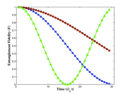
We now proceed to illustrate and discuss some representative numerical results, for a generic qubit Hamiltonian of the form $H=\Omega_{z}\sigma_{z}+\varepsilon_{x}\sigma_{x}+\varepsilon_{y}\sigma_{y}$. First, we compare the SelDD with the FDD protocol in the presence of a finite interpulse separation $\Delta t$ (which is the control non-ideality we focus on). From Eq. (26), the free evolution corresponds to entanglement fidelity

$${\cal F}(T)=\cos(\Omega T)^{2}\,,\;\;\Omega\approx\Omega_{z}\,.$$

A typical behavior is depicted in Figure 1. The changes in the oscillation frequency, $\Omega\mapsto\varepsilon_{x}$, $\Omega\mapsto\varepsilon_{y}$, associated with each SelDD protocols, are clearly seen. Not only does FDD display better performance for comparable, fixed $\Delta t$, but it also turns out to be less sensitive to errors in the estimate of the Hamiltonian. In fact, the FDD protocol exhibits better performance as the norm of the estimation error grows.

Figure 1: Comparison between selective DD protocols: (color online) FDD (brown, circles) and SelDD, with $\sigma_{x}$ (blue, squares) or $\sigma_{y}$ (green, triangles) pulses. Symbols are displayed every four decoupling cycles to improve readability. Brown and blue curves correspond to oscillations of the form ${\cal F}(T)=\cos(\varepsilon_{x,y}T)^{2}$, respectively – as following from Eq. (26) for the selectively decoupled evolution. Actual Hamiltonian: $H=\Omega_{z}\sigma_{z}+\varepsilon_{x}\sigma_{x}+\varepsilon_{y}\sigma_{y},$ $\varepsilon_{x}=\Omega_{z}/20,\varepsilon_{y}=\Omega_{z}/10.$ The estimated Hamiltonian is proportional to $\sigma_{z}$. $\Omega T=30$, $\Omega_{z}\Delta t=0.04.$

In comparing maximal DD strategies, we made sure to employ in each case the appropriate choice of control pulses, as following from the analysis of the higher-order corrections presented above. Different control scenarios were investigated. The main features emerging from our study may be summarized as follows.

As the parameter $\Delta t$ grows within the parameter range considered, all protocols move away from the ideal behavior in a regular fashion: Overall, the best performance is attained by the FED strategy, followed by MaxDD. The DEF strategy, where we use the feedback loop to correct the main, estimated Hamiltonian, shows a sensible reduction of the performance for longer $\Delta t$, making MaxDD more effective in the long time regime. Independent tests confirmed that this implementation is more sensitive to the $\Delta t$ parameter increasing. For sufficiently small $\Delta t$, DEF can outperform the maxDD, however, compared to FED, it looses its advantage soon.

For a fixed value of both $\Delta t$ and $T$, we also investigated the performance of the above protocols when the norm of the estimation error on the Hamiltonian is increased. The same comparative results are found, with fairly uniform behavior, and no particular crossings.

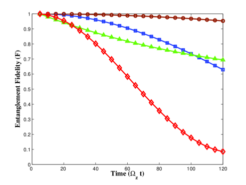
Based on the above analysis, the most robust and information-efficient strategy turns out to be the symmetrized FED protocol, that is, the feedback-corrected version of a symmetric selective DD. It is worth to notice that the symmetrization on nested SelDD is crucial in determining such advantage: The non-symmetrized version does not succeed, in general, at outperforming the open-loop strategy. We summarize in Figure 2 the typical behavior of the protocols under considerations for a fixed $\Delta t$ value. We show also the simulation results for a FED strategy with a non-symmetrized nested SelDD, clearly supporting the above claim on the importance of symmetrization.

Figure 2: Comparison between maximal DD protocols: (color online) MaxDD (blue, squares), symmetrized FED (brown, circles), non-symmetrized FED (green, triangles), DEF (red, diamonds). Symbols are displayed every two decoupling cycles to improve readability. Actual Hamiltonian: $H=\Omega_{z}\sigma_{z}+\varepsilon_{x}\sigma_{x}+\varepsilon_{y}\sigma_{y},$ $\varepsilon_{x}=\varepsilon_{y}=\Omega_{z}/10.$ The estimated Hamiltonian is proportional to $\sigma_{z}.$ $\Omega_{z}T=120,\Omega_{z}\Delta t=0.32.$

VI Discussion and Conclusion

We have designed and characterized different quantum procedures for exploiting single-bit classical feedback as a tool for quantum dynamical averaging – applicable alone or in conjunction with traditional (deterministic) open-loop decoupling methods. Beside providing general (linear-algebraic) necessary and sufficient conditions for a two-step averaging processes to be implementable in principle via single-bit feedback on an arbitrary finite-dimensional open quantum system, our analysis points to novel possibilities for successfully merging open- and closed-loop techniques toward achieving robust quantum dynamical control. In particular, the concatenated feedback-enhanced decoupling protocol proposed and discussed for a two-dimensional target system in Sections IV-V is found to exhibit better performance than its open-loop counterpart, the best possible maximal DD scheme with respect to the estimated interaction. For higher dimensional systems, the integration of discrete-time feedback with open-loop decoupling schemes appears more delicate, as the constraints imposed by Theorem 2 become more demanding. While it is still conceivable in principle to employ feedback to enhance the performance of selective open-loop strategies, especially whenever uncertainty is limited or it affects the free evolution in some structured fashion, further investigation is needed to address the relevant issues in detail.

From an information-theoretic perspective, our results offer some suggestive insights on the role played by classical information in various quantum control schemes. While different schemes become essentially equivalent and insensitive to system’s parameters in the ideal limit of arbitrarily fast control, prior information on the underlying Hamiltonian plays a central role in the optimization of different protocols as soon as parameter uncertainties become important and non-ideal control settings are considered – as it is unavoidably the case in practice. Thus, the role of information in control design and synthesis cannot be underestimated. Interestingly, even if purely open-loop maximal decoupling schemes may be optimized by using the initial estimation, they do not allow any improvement in the estimate itself. Thus, the full power of a feedback strategy might is expected to appear in adaptive control settings, like the simple Hamiltonian estimation setting presented in Section IV.3.

From yet another standpoint, the proposed feedback-concatenated protocols further support the relevance of hybrid strategies for robust quantum dynamical control Byrd et al. (2004). In particular, our results take an additional step toward establishing the potential of dynamical decoupling methods for integration with existing passive and active quantum control techniques – following the demonstration of concatenated quantum error correction and decoupling codes Boulant et al. (2002), the development Wu and Lidar (2002); Byrd and Lidar (2002); Viola (2002) and implementation of decoherence-free encoded dynamical decoupling schemes Fortunato et al. (2002), and the recent development of fault-tolerant, concatenated dynamical decoupling protocols Khodjasteh and Lidar (2005). Beside, as mentioned earlier, generalizations of the proposed framework to higher-dimensional systems and ancillas, additional extensions to include non-ideal measurement and realistic control capabilities are certainly necessary for a more complete picture and possible contact with experiment to be established. At the formal level, we expect that linear-algebraic tools may continue to prove useful in that respect, along with general methods from quantum fault-tolerance theory. In practice, although meeting all the relevant control requirements appears demanding by present capabilities, the kind of operations needed for the proposed hybrid feedback-decoupling protocols have already been implemented separately in different device settings exp (2005) (see also discussion in Lloyd et al. (2004)), and experimental progress is steady. In this respect, it might be especially intriguing and timely to explore possible proof-of-principle applications in scalable devices based on trapped ions, where quantum error correction has been recently demonstrated Chiaverini et al. (2004) and different isotopic species could be used in principle for system and ancilla degrees of freedom Blinov et al. (2002), or semiconductor quantum dots, where suggestive proposals for controlling a slowly fluctuating mesoscopic spin environment via a suitable probe spin already exist Tay .

Lastly, the analysis of higher order corrections, as carried out in Section V, may be seen as a simple instance of the sensitivity minimization problem, which is one of the fundamental problems of robust control theory. In this perspective, it is our hope that the present work will stimulate further exploration and input from classical control theory, as well as the quantum control and system engineering communities.