Optimal quantum circuits for general phase estimation

Abstract

We address the problem of estimating the phase $\phi$ given $N$ copies of the phase rotation gate $u_{\phi}$. We consider, for the first time, the optimization of the general case where the circuit consists of an arbitrary input state, followed by any arrangement of the $N$ phase rotations interspersed with arbitrary quantum operations, and ending with a POVM. Using the polynomial method, we show that, in all cases where the measure of quality of the estimate $\tilde{\phi}$ for $\phi$ depends only on the difference $\tilde{\phi}-\phi$, the optimal scheme has a very simple fixed form. This implies that an optimal general phase estimation procedure can be found by just optimizing the amplitudes of the initial state.

The possibility of encoding information into the relative phase of quantum systems is often exploited in several quantum information processing tasks and several kinds of applications. For example, it was shown that in most existing quantum algorithms the information to be retrieved after the computation is contained in relative phases CEMM . Moreover, information is encoded into phase properties in some quantum cryptographic protocols BB84 , and in some precision measurements, such as the schemes on which atomic clocks are based atclocks . Therefore, the issue of estimating the phase in the most efficient way is of great interest.

We phrase the phase estimation problem as follows. Let $u_{\phi}$ be a single qubit gate that, in a prescribed ‘computational’ basis $\{|0\rangle,|1\rangle\}$ maps the state $|0\rangle$ to $|0\rangle$ and $|1\rangle$ to ${\mathrm{e}}^{{\mathrm{i}}\phi}|1\rangle$. We assume we have no prior knowledge about $\phi$. The objective is to estimate $\phi$ using some procedure that will output some guess $\tilde{\phi}$. We characterize the quality of a estimate by a “cost function” $C(\phi,\tilde{\phi})$, which specifies the penalty associated with guessing $\tilde{\phi}$ when the actual phase is $\phi$. We are given $N$ identical single qubit quantum gates $u_{\phi}$, and the goal is to use these gates along with any other operations in order to produce an estimate of $\phi$. The optimal procedure is the one that has the minimum expected cost.

Most of the previous work on phase estimation assumes some fixed state encoding the phases, and the only thing to be optimized is the final POVM measurement helstrom ; holevo77 ; dbe . More recent work DDEMMb fixes the way the phase gates are applied and optimizes the choice of input state and final POVM.

The crucial point is that in this paper we are not restricted to preparing some input state, then applying all of the phase rotations, and then performing an optimal POVM. We consider, for the first time, the case where one has full freedom over how to use the phase rotation gates in an experiment designed to optimally estimate the phase. Any realistic experiment of this type can be viewed as computation, completely specified by a quantum circuit acting on some finite number of qubits and involving, apart from the $N$ copies of the $u_{\phi}$ gates, some finite number of arbitrary quantum gates of our choice. In fact, many quantum algorithms, including Shor’s quantum algorithm for factoring integers, can be phrased in terms of such phase estimations kitaev ; CEMM . This has originally provided motivation for this work.

We assume the phase $\phi$ is chosen uniformly from $[0,2\pi)$ and that a suitable quantum circuit containing $N$ copies of the $u_{\phi}$ gates outputs some value $y$ with probability ${\mathrm{Pr}}(y|\phi)$. From $y$ we infer, following a prescribed rule, the estimate $\tilde{\phi}_{y}$. The quality of the whole procedure is quantified by the expected cost $\bar{C}$, given by

$$\bar{C}=\frac{1}{2\pi}\sum_{y}{{\int_{\phi=0}^{2\pi}{d\phi{\mathrm{Pr}}(y|\phi)\cdot C(\phi,\tilde{\phi}_{y})}}}.$$ (1)

The next part of this paper describes a very simple procedure for estimating $\phi$, that only requires one to optimize the choice of initial state to an otherwise fixed procedure. The rest of the paper then reduces the very general case we have described above to this very simple case.

For a given cost function, the quality of an estimation procedure depends on both ${\mathrm{Pr}}(y|\phi)$ and the inference rule $y\mapsto\tilde{\phi}_{y}$. The optimal protocol gives the minimum possible average $\bar{C}$. We restrict attention to cost functions $C$ that depend only on $\phi-\tilde{\phi}_{y}$, and therefore adopt the notation $C(\phi,\tilde{\phi}_{y})=C(\phi-\tilde{\phi}_{y})$. We will make only the following very weak assumption on the cost function (which corresponds to a more general class of cost functions than the “Holevo” class that is typically considered holevo )

$$\int_{\phi=0}^{2\pi}{d\phi|C(\phi)|}<\infty.$$ (2)

We will deal with specific cost functions later on.

Let us start by describing a simple and natural approach for estimating the phase $\phi$, illustrated in Figure 1.

Procedure 1

• Prepare $m$ qubits in state $|x\rangle=\sum_{j=0}^{N}\alpha_{j}|j\rangle$, with $N\leq 2^{m}-1$. The exact values of $\alpha_{j}$ depend on the cost function to be maximized.

• Apply the $u_{\phi}$ gates to effect $U_{\phi}$

  $$U_{\phi}\sum_{j=0}^{N}\alpha_{j}|j\rangle=\sum_{j=0}^{N}\alpha_{j}{\mathrm{e}}^{{\mathrm{i}}j\phi}|j\rangle.$$ (3)

• Apply the inverse quantum Fourier transform to obtain

  $$2^{-m/2}\sum_{y=0}^{2^{m}-1}\left(\sum_{j=0}^{N}\alpha_{j}{\mathrm{e}}^{{\mathrm{i}}j(\phi-\mbox{$\frac{2\pi y}{2^{m}}$})}\right)|y\rangle,$$ (4)

  measure $y$ and calculate the estimate $\tilde{\phi}_{y}=\mbox{$\frac{2\pi y}{2^{m}}$}$.

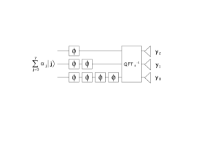
Figure 1: A simple approach for estimating $\phi$, in the case that $N=7$. Optimizing over the input amplitudes $\alpha_{j}$, produces an optimal estimate of $\phi$.

The surprising claim is the following. Given any function $C$ satisfying Eq. (2), the minimum of $\bar{C}$ obtained by optimizing the $\alpha_{j}$ in Procedure 1 is the infimum of all values obtainable by any realistic experiment (as we described above and illustrate in Figure 2). It is important to also note that apart from the preparation of the initial state, the above procedure can be implemented using the $N$ black boxes $u_{\phi}$ and a number of elementary gates polynomial in $\log(N)$. Efficient preparation of states is discussed in km . Exact implementation of quantum Fourier transforms is discussed in mz , and arbitrarily good approximations are discussed in kitaev ; hh .

The remainder of this paper will prove this claim by a sequence of reductions.

Let us start with a very general circuit (Figure 2) which uses $m+d$ qubits, where $m$ and $d$ can be arbitrarily large. The first $m$ qubits are measured after the computation, yielding the output $0\leq y\leq 2^{m}-1$, whereas the remaining $d$ qubits are discarded.

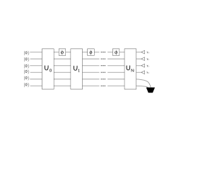
Figure 2: Most general approach for estimating the unknown phase rotation. This subsumes Procedure 1, as well as more complicated procedures with classical feedback.

Since we are allowing arbitrarily many extra “ancilla” qubits, and since any classical feedback scheme can in principle be implemented by a unitary operation using a sufficiently large ancilla, the family of schemes that can be implemented by a quantum circuit of this form includes any scheme using finite dimensional state spaces.

For convenience, we let the output $y$ correspond to the phase estimate $\tilde{\phi}_{y}=\mbox{$\frac{2\pi y}{M}$}$, for some $M$, $M\leq 2^{m}$. For a fixed approximation scheme (using finite means) and cost function satisfying Eq. (2), and assuming a uniform prior distribution of the $\phi$, this simplifying assumption will give us a scheme with expected cost that is at most $\bar{C}+\epsilon_{M}$, where $\epsilon_{M}\rightarrow 0$ as $M\rightarrow\infty$, and $\bar{C}$ is the lowest expected cost for any possible scheme. Thus the infimum of the $\bar{C}$ over all such restricted schemes equals the infimum of the $\bar{C}$ over all possible such schemes.

In fact we will also show later that as long as $M\geq N+1$, this simplifying assumption does not cost us anything. That is, the infimum of the expected costs of all the schemes using the inference rule $y\mapsto\frac{2\pi y}{M}$ for any $M\geq N+1$ is the infimum of the possible expected costs using any inference rule $y\mapsto\tilde{\phi}_{y}$.

Suppose we came up with a general circuit that performs an estimation of $\phi$ according to some prescribed set of criteria. Let us first show that such a circuit is equivalent, for our purposes, to another one, which has much simpler structure.

The state at the output of the circuit can be written as

$$\sum_{y=0}^{M}\sum_{z=0}^{2^{d}-1}\alpha(y,z,\phi)|y\rangle|z\rangle,$$ (5)

where each amplitude $\alpha(y,z,\phi)$ is a polynomial in ${\mathrm{e}}^{{\mathrm{i}}\phi}$ of degree at most $N$

$$\alpha(y,z,\phi)=\sum_{j=0}^{N}\frac{\alpha_{j}(y,z)}{\sqrt{M}}{\mathrm{e}}^{{\mathrm{i}}j\phi}.$$ (6)

This fact follows just as in BBCMW where the polynomial method is applied to an oracle revealing one of many Boolean variables. This paper is the first time the polynomial method is applied to oracles with continuous variables. Since we assume that the cost function is of the form $C(\phi,\tilde{\phi}_{y})=C(\phi-\tilde{\phi}_{y})$, then we can also assume, without loss of generality that the optimal conditional probability

$${\mathrm{Pr}}(y|\phi)=\sum_{z}|\alpha(y,z,\phi)|^{2}$$ (7)

depends only on the difference $\phi-\mbox{$\frac{2\pi y}{M}$}$ and therefore equals

$${\mathrm{Pr}}(0|\phi-2\pi y/M)=\sum_{z}|\alpha(0,z,\phi-2\pi y/M)|^{2}.$$ (8)

To simplify the notation, we let $\alpha_{j}(z)=\alpha_{j}(0,z)$. Therefore, a circuit that produces amplitudes

$$|\alpha(y,z,\phi)|=\frac{1}{M}|\sum_{j=0}^{N}\alpha_{j}(z){\mathrm{e}}^{{\mathrm{i}}j(\phi-\mbox{$\frac{2\pi y}{M}$})}|$$ (9)

also leads to the optimal estimation of $\phi$. Thus the following simple estimation procedure, whose circuit is illustrated in Figure 3, performs equally well:

• Prepare $m+d$ qubits in state $|x\rangle=\sum_{z=0}^{2^{d}-1}\sum_{j=0}^{N}\alpha_{j}(z)|j\rangle|z\rangle$. For this preparation to be possible $m$ has to be chosen such that $N<2^{m}$.

• Apply the $u_{\phi}$ gates to effect $U_{\phi}$ on the first $m$ qubits

  $$U^{N}_{\phi}\sum_{z=0}^{2^{d}-1}\sum_{j=0}^{N}\alpha_{j}(z)|j\rangle|z\rangle = \sum_{z=0}^{2^{d}-1}\sum_{j=0}^{N}\alpha_{j}(z){\mathrm{e}}^{{\mathrm{i}}j\phi}|j\rangle|z\rangle.$$ (10)

• Apply the inverse quantum Fourier transform, $|j\rangle\mapsto(1/{\sqrt{M}})\sum_{y=0}^{M-1}{{\mathrm{e}}^{-{\mathrm{i}}\mbox{$\frac{2\pi y}{M}$}}|y\rangle}$, to obtain

  $$\frac{1}{\sqrt{M}}\sum_{z=0}^{2^{d}-1}\sum_{y=0}^{M-1}\left(\sum_{j=0}^{N}\alpha_{j}(z){\mathrm{e}}^{{\mathrm{i}}j(\phi-\mbox{$\frac{2\pi y}{M}$})}\right)|y\rangle|z\rangle,$$ (11)

  and measure $y$.

The following two observations lead to further simplifications.

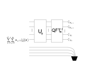
Figure 3: Without loss of generality, we can assume our phase estimation procedure has the form illustrated in this figure, where $2^{m}\geq M\geq N+1$. The top register contains $m$ qubits, and the bottom $d$ qubits are ancilla qubits that may be entangled with the first $m$ qubits, but are discarded.

Let us first notice that in this procedure the role of the $d$ auxiliary qubits is restricted to the initial preparation of the most general state of the first $m$ qubits (all subsequent operations are restricted to these $m$ qubits). Usually, such a state is described by a density operator which can always be expressed as a mixture of pure states of the first $m$ qubits. The average cost in this case is given by the average, over the mixture, of individual expected costs pertaining to the pure states in the mixture. Thus the expected cost for the mixture cannot be greater than all of the individual expected costs for the contributing pure states; hence either some of the contributing costs are greater or they are all equal. In either case a judicial choice of a pure state of the $m$ qubits leads to equally good or better phase estimation. This argument implies that without loss of generality we can restrict our circuit to only $m$ qubits (plus some ancilla bits used to implement $U_{\phi}^{N}$ using $N$ copies of $u_{\phi}$) and run the estimation on pure states.

Secondly, in the description above the quantum Fourier transform is parameterized by $M$, where $N+1\leq M\leq 2^{m}$, but in fact any $M\geq N+1$, in particular $M=2^{m}$, will work equally well. To see this consider a cost function of the form $C(\phi-\tilde{\phi}_{y})$. The expected cost, for some $M$, is

$$\bar{C} = \frac{1}{2\pi M}{{\int_{\phi=0}^{2\pi}d\phi\sum_{y=0}^{M-1}{\left|\sum_{j=0}^{N}\alpha_{j}{\mathrm{e}}^{{\mathrm{i}}j(\phi-\mbox{$\frac{2\pi y}{M}$})}\right|^{2}C(\phi-\mbox{$\frac{2\pi y}{M}$})}}}$$

$$= \frac{1}{2\pi M}\sum_{y=0}^{M-1}{{\int_{\phi^{\prime}=0}^{2\pi}d\phi^{\prime}{\left|\sum_{j=0}^{N}\alpha_{j}{\mathrm{e}}^{{\mathrm{i}}j\phi^{\prime}}\right|^{2}C(\phi^{\prime})}}}$$

$$= \frac{1}{2\pi}{{\int_{\phi^{\prime}=0}^{2\pi}d\phi^{\prime}{\left|\sum_{j=0}^{N}\alpha_{j}{\mathrm{e}}^{{\mathrm{i}}j\phi^{\prime}}\right|^{2}C(\phi^{\prime})}}},$$

where $\phi^{\prime}=\phi-\mbox{$\frac{2\pi y}{M}$}$. The expected cost does not depend on $M$ as long as $M\geq N+1$.

Recall that we mentioned in the introduction that as $M\rightarrow\infty$ the difference between the optimal $\bar{C}$ assuming the inference rule $y\mapsto\tilde{\phi}_{y}=\frac{2\pi y}{M}$ and the optimal $\bar{C}$ without such an assumption is $\epsilon_{M}\rightarrow 0$. Since we have just shown that for all $M\geq N+1$, the expected cost $\bar{C}$ is constant, this means that the difference $\epsilon_{M}$ is in fact $0$ once $M\geq N+1$. In other words, assuming $\tilde{\phi}_{y}=\frac{2\pi y}{M}$ does not cost us anything as long as we use $M\geq N+1$.

It is clear that the exact value of the expected cost now depends only on the $\alpha_{j}$ values, that is, on the initial state, which means that given a specific cost function all we have to do is to choose an optimal initial state.

We emphasise that the schemes in Figs. 1 and 2 provide an optimal covariant estimation scheme even for general cost functions not necessarily of the Holevo class. Indeed, in DDEMMb it is proved that there exists a discrete POVM achieving the same average cost of any covariant continuous POVM. By the Naimark theorem helstrom this means that there exists an orthogonal measurement on the system and an ancilla achieving the discrete POVM, and a further extension allows to have the POVM as rank-one (projectors of rank $r>1$ can be easily connected to rank-one projectors via a suitable controlled-unitary interaction with an ancilla).

Let us now address the problem of optimal input states for two different cost functions. First we look at the minimization of the “$1-$Fidelity” cost function $C_{F}(\phi,\tilde{\phi}_{y})=\sin^{2}[(\phi-\tilde{\phi}_{y})/2]$. The minimum cost is achieved with the initial state

$$|x_{N}^{\mathrm{optimal}}\rangle = \sum_{j=0}^{N}{\sqrt{\mbox{$\frac{2}{N+2}$}}\sin\left({\mbox{$\frac{(j+1)\pi}{N+2}$}}\right)|j\rangle}.$$ (12)

The error in fidelity of this protocol goes to zero according to the square of the number of black boxes used $\bar{C}_{F}=O(1/N^{2})$. It is interesting to note that the fidelity of the more conventional approach to phase-rotation estimation with the uniform initial state ($\alpha_{j}=\mbox{$\frac{1}{\sqrt{N+1}}$}$ for all $j$) only tends to zero linearly in $N$. That is $\bar{C}_{F}=\Omega(1/N)$.

Another cost function that is commonly used is the window function that allows any error smaller than $\delta$: $C_{W}^{\delta}(\phi,\tilde{\phi})=0$ if $|\phi-\tilde{\phi}|<\delta$, but $C_{W}^{\delta}(\phi,\tilde{\phi})=1$ if $|\phi-\tilde{\phi}|\geq\delta$. The minimisation of this cost leads to optimal states with amplitudes $\alpha_{j}=1/\sqrt{N+1}$, which corresponds to what is effectively used by Shor’s algorithm shor ; kitaev ; CEMM , and provides an expected cost in $O(\frac{1}{\delta N})$.

In this paper we have addressed the general problem of finding the optimal estimating procedure for the real parameter $\phi$ given $N$ copies of the single qubit phase rotation $u_{\phi}$ within a general quantum circuit in finite dimensions. We considered the general case where the circuit consists of an arbitrary input state followed by any arrangement of the $N$ phase rotations interspersed with arbitrary quantum operations. The main result was the proof that in all cases, and for any covariant cost function, we want to use the optimal phase estimation procedure is equivalent to a quantum Fourier transform in an appropriate basis.

Our result is very general, and gives a recipe for finding the best achievable phase estimation for a given cost function. In practice, once we know the minimum cost possible, one can also search for and use easier-to-implement phase estimation procedures that achieve the same, or similar expected cost. Due to the generality of our main result, it will surely find many other interesting applications in physical and computational scenarios.

This is the first application of the polynomial method to “black-boxes” encoding continuous variables, in this case, one real parameter. The method can also be applied to several real parameters, as well as combinations of real and discrete parameters.

References

- (1) R. Cleve, A. Ekert, C. Macchiavello, and M. Mosca, Proc. R. Soc. London, Ser. A 454, 339 (1998).
- (2) C. H. Bennett and G. Brassard, in Proceedings of the IEEE International Conference on Computers, Systems, and Signal Processing, Bangalore, India, 1984, pp. 175–179.
- (3) See for example D.J. Wineland et al., IEEE Trans. on Ultrasonics, Ferroelectrics and Frequency Control A 37, 515 (1990).
- (4) Robert Beals, Harry Buhrman, Richard Cleve, Michele Mosca, Ronald de Wolf. Journal of the ACM (2001), Vol. 48, No. 4, 778-797.
- (5) C. W. Helstrom, Quantum detection and estimation theory, Academic Press, New York, 1976.
- (6) A.S. Holevo, Probabilistic and statistical aspects of quantum theory, North Holland (Amsterdam, 1982).
- (7) This class of mixed states is characterised by the restriction that the elements of have fixed phase along the diagonals, i.e. . In this case the optimal is given by .
- (8) I.S. Gradshteyn and I.M. Ryzhik, Table of Integrals, Series and Products (fourth edition, Academic Press, San Diego, 1965).
- (9) R. Derka, V. Buzek, A. Ekert, Phys. Rev. Lett. 80, 1571 (1998).
- (10) C. W. Gardiner, Quantum Noise (Springer–Verlag, Berlin 1991).
- (11) L. Hales, S. Hallgren. In Proceedings of the 41st Annual Symposium on Foundations of Computer Science, (2000) 515–525.
- (12) P. Kaye, M. Mosca. Proceedings of the International Conference on Quantum Information, OSA CD-ROM (Optical Society of America, Washington, D.C., 2002), PB28.
- (13) M. Mosca, C. Zalka. International Journal of Quantum Information, Vol. 2, No. 1 (2004) 91-100.
- (14) P. Shor. SIAM J. Computing, 26:1484-1509, 1997.
- (15) A. Y. Kitaev, Russ. Math. Surv., 52(6):1191-1249, 1998.
- (16) A.S. Holevo, Reports on Mathematical Physics, 13(3), 1978.
- (17) W. van Dam, G. M. D’Ariano, A. Ekert, C. Macchiavello, M. Mosca, manuscript in preparation.