Optical gratings induced by field-free alignment of molecules

Abstract

We analyze the alignment of molecules generated by a pair of crossed ultra-short pump pulses of different polarizations by a technique based on the induced time-dependent gratings. Parallel polarizations yield an intensity grating, while perpendicular polarizations induce a polarization grating. We show that both configurations can be interpreted at moderate intensity as an alignment induced by a single polarized pump pulse. The advantage of the perpendicular polarizations is to give a signal of alignment that is free from the plasma contribution. Experiments on femtosecond transient gratings with aligned molecules were performed in CO₂ at room temperature in a static cell and at 30 K in a molecular expansion jet.

I Introduction

Excitation with non-resonant high power laser pulses has become a powerful technique for preparing aligned molecules Stap . With ultra-short laser pulses, typically of less than 100 fs pulse duration, molecules periodically realign after the pump extinction, showing revivals in the observed signal. Various methods are employed to measure such post-pulse molecular alignment. They make use either of ionization-fragmentation combined with an imaging technique Stap ; Sakai or of non-linear optical properties Renard2003 ; Renard2005 . In the methods of the latter category, the depolarization or the spatial deformation of a probe pulse is measured as a function of time elapsed after the aligning pulse. The effect is based on the time-dependent non-linear contribution of alignment to the refractive index Renard2003 ; Renard2005 . Transient grating experiments have been also performed to explore alignment of molecules Comstock ; Stavros . In these experiments, a transient grating was produced by two synchronized pump pulses, and the amount of light diffracted from a third probe pulse was recorded at different delays. It appeared that the recorded signal exhibited the same time behavior than other alignment signals, i.e. confirming the detection of post-pulse molecular alignment. As in Refs. Renard2003 ; Renard2005 a deformation of the measured signal with increasing intensity has been noted. Whereas in Ref. Comstock , the change in the shape of the revivals has been attributed to molecular changes and the apparition of a constant background due to ionization and plasma formation, a more likely explanation for this modification of DFWM transient shapes has been suggested Lavorel : the background is due to permanent alignment and the alteration of revivals is a consequence of heterodyning with this background. In fact, this had been already pointed out for all experiments with homodyne detection Renard2003 . Stavros et al. Stavros corroborated this explanation in the case of DFWM for O₂ molecules. At the highest intensity investigated in Ref. Stavros , the possible contribution of an ion grating has also been suggested.

The aim of the present work is to investigate the mechanisms involved in high intensity DFWM experiments by using two types of gratings (intensity or polarization grating) produced by two crossed beams. Furthermore, it will be shown that quantitative measurement of alignment with both configurations is possible with this technique.

II Experimental setup

The experimental setup uses the well known femtosecond degenerate four-wave mixing technique (DFWM) also called femtosecond transient grating spectroscopy Brown . It consists of exciting the molecular sample by two synchronized pump pulses at 800 nm (pulse duration of 90 fs) focused and crossed at a given angle $\Theta$ (Fig.1). They are both derived from a chirped pulse amplified Ti:Sapphire system working at 20 Hz. The energy and the polarization direction of the two pump pulses are controlled by means of a half-wave plate and a polarizer. A third probe pulse, time delayed with respect to the pumps, is mixed with the others. The probe beam sees a transient grating and is diffracted. The amount of diffracted light is monitored as a function of the time delay with a photomultiplier. The sample is a CO₂ gas, either at room temperature in a static cell, or in a molecular supersonic jet for lower rotational temperatures. Both beams are focused and collimated with $f=300$ mm lenses. It is noticed that, like in other all-optical methods, DFWM gives the opportunity to work with a good sensitivity in a wide pressure range (typically from 1 mbar to a few bars). The role of the two pump pulses is to excite the rotational coherence of the molecules. Two different experiments have been performed which correspond to parallel and perpendicular polarizations of the pump pulses. The two cases are treated separately in the next sections.

III Theory

III.1 Parallel polarizations: linear total polarization, intensity grating

We consider a simplified model for the formation of the grating. We assume two plane waves, with wavelength $\lambda$, propagating in the $(x,z)$ plane with wave vectors $(-k_{x},0,k_{z})$ and $(k_{x},0,k_{z})$ (see Fig. 1). The small cross-angle between the two pump beams is given by $\sin(\Theta/2)=k_{x}\lambda/2\pi\approx\Theta/2$. With two pump pulses polarized along the $y$-axis (of vector unit $\vec{e}_{y}$), an intensity grating is formed with a total electric field periodically modulated along the $x$-axis: $\vec{E}_{\text{pump}}=2E_{p}(t)\cos(k_{x}x)\cos(\omega t-k_{z}z)\vec{e}_{y}$, where $E_{p}(t)$ is the pump field envelope (taken the same for both fields). We are facing therefore the case of molecules interacting with a non resonant linearly polarized laser field, which has been extensively studied (see Ref. Stap and references therein). The additional ingredient is the spatial modulation of the total intensity. If we consider a weak probe pulse polarized parallel to the pumps ($y$-axis) and which propagates with the wave vector $(-k_{x},0,k_{z})$, the only component of the induced dipole at a position $\vec{r}=(x,y,z)$ whose expectation value does not average out is the $y$-component :

$$\langle\vec{\mu}_{\text{ind}}\rangle_{\vec{r},t} = \left[\bar{\alpha}+\Delta\alpha\left(\langle\cos^{2}\theta_{y}\rangle_{\vec{r},t}-1/3\right)\right]$$ (1)

$$\times E_{\text{probe}}(t)\cos(\omega t+k_{x}x-k_{z}z)\vec{e}_{y},\quad$$

where $\bar{\alpha}$ is the mean polarizability, $\Delta\alpha=\alpha_{\parallel}-\alpha_{\perp}$ is the difference of polarizability parallel and perpendicular to the molecular axis, $E_{\text{probe}}(t)$ is the probe envelope, and $\theta_{y}$ is the angle between the molecular axis and the common polarization direction ($y$-axis). The expectation value $\langle\cos^{2}\theta_{y}\rangle_{\vec{r},t}$ is a measure of alignment and is a function of the total pump intensity at the position $\vec{r}$. Consequently, it has the same spatial period as the total intensity. It also depends on the time delay between the pump and probe pulses. The signal electric field measured by the photo-detector is then obtained by summation over the interaction volume of spherical waves radiated by the dipole. The first term of the right hand side of Eq. (1) describes the effect of the linear index of refraction on the probe beam and is not interesting for our purpose. The second term is periodic and leads to constructive interference along symmetric phase-matching directions $x/z=(2n-1)k_{x}/k_{z}$, with $n$ the diffraction order. Only the order 1 is considered experimentally (see Fig. 1). The experimental signal measured at a position $\vec{r_{0}}$, proportional to the modulus squared of the total electric field, is interpreted as the diffraction of the probe beam by the transient grating produced by the pumps

$$I_{\text{sig}}(\vec{r_{0}},t)\propto|\vec{E}_{\text{sig}}(\vec{r_{0}},t)|^{2}\propto|\int\int\int_{V}dr{\cal R}[\vec{E}_{\text{rad}}(\vec{R},t)]|^{2},$$ (2)

with $\vec{E}_{\text{rad}}$ the spherical electric field radiated by the dipole moment

$$\vec{E}_{\text{rad}}(\vec{R},t)=\frac{k^{2}}{4\pi\epsilon_{0}}\langle\vec{\mu}_{\text{ind}}\rangle_{\vec{r},t}\ \frac{e^{ikR}}{R}$$ (3)

and with $\vec{R}=\vec{r_{0}}-\vec{r}$, $x/x_{0},y/y_{0},z/z_{0}\ll 1$, $k\simeq\omega/c$.

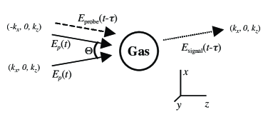
Figure 1: Experimental scheme for transient grating experiments (see text). $E_{p}$ and $E_{\text{probe}}$ are respectively the pump and probe field envelope. The diffracted signal field envelope is $E_{\text{signal}}$ .

At low and moderate intensities (i.e. below the saturation of alignment), numerical simulations show that $\langle\cos^{2}\theta_{y}\rangle_{\vec{r},t}-1/3$ is approximately proportional to the total pump intensity $4I_{0}\cos^{2}(k_{x}x)=2I_{0}(1+\cos 2k_{x}x)$, where $I_{0}$ is the peak intensity of a single pump (see Appendix A.1). The constant term 2$I_{0}$ corresponds to the zeroth order of diffraction and is responsible for nonlinear variation of the refractive index seen by the probe pulse. The second term 2$I_{0}\cos 2k_{x}x$ leads to diffraction orders $n=\pm 1$. It is shown in Appendix A.1 that :

$$\langle\cos^{2}\theta_{y}\rangle_{\vec{r},t}-1/3\approx\left(\langle\cos^{2}\theta_{y}\rangle_{t}-1/3\right)(1+\cos 2k_{x}x),$$ (4)

with

$$\langle\cos^{2}\theta_{y}\rangle_{t}-1/3\approx 2\xi_{0}[\delta+\kappa f(t)],$$ (5)

and

$$\xi_{0}=\Delta\alpha/4\hbar\int dtE_{p}^{2}(t),$$ (6)

the intensity area of a single pump. $\langle\cos^{2}\theta_{y}\rangle_{t}$ corresponds to the alignment that would be induced by a single linearly polarized pulse of intensity $2I_{0}$. For a given molecule and temperature, $\delta$ and $\kappa$ are constant ($\delta\text{ and }\kappa\to 0$ at low intensity), and $f(t)$ is a specific function independent of $\xi_{0}$. The summation over the volume (Eq.(2)) gives a signal of intensity :

$$I_{\text{sig}}(t)\propto\left(\langle\cos^{2}\theta_{y}\rangle_{t}-1/3\right)^{2},$$ (7)

where the spatial dependence has now disappeared. The measured signal (order 1) can thus be calculated for any pump-probe time delay, solving the time-dependent Schrödinger equation Renard2003 using a single linearly polarized pump beam of intensity $2I_{0}$. This takes into account the fact that the spatial distribution of the total intensity is modulated between 0 and $4I_{0}$.

In other words, the sample of aligned molecules presents a nonlinear index of refraction, which depends on the pump intensity. As the intensity along the grating is modulated by optical interferences, a spatial modulation of refractive index is formed. This gives a refractive index grating and a signal directly related to the post-pulse alignment, as shown by Eq. (7).

III.2 Perpendicular polarizations: elliptic total polarization, polarization grating

For perpendicular polarizations, with one pump aligned at $-45^{\circ}$ and the other at $+45^{\circ}$ with respect to the $y$-axis, the resulting field is in general elliptically polarized. The state of polarization of the total pump electric field depends on the spatial position and alternates between linear and circular, forming a polarization grating. In a grating period, the total electric field varies from linear (along the $y$-axis), circular (right), linear (along the $x$-axis), to circular (left), with intermediate elliptic polarizations. Furthermore, its magnitude varies periodically along the $x$-coordinate and is maximum for the linear polarization and minimum for the circular one. Since $\Theta$ is a small angle, the total pump field is indeed polarized in the $(x,y)$ plane as

$$\vec{E}_{\text{pump}} = \sqrt{2}E_{p}(t)[A(x)\sin(\omega t-k_{z}z)\vec{e}_{x}$$ (8)

$$+B(x)\cos(\omega t-k_{z}z)\vec{e}_{y}]$$

with $A(x)=\pm\sin(k_{x}x)$, $B(x)=\cos(k_{x}x)$, and $E_{p}(t)$ the pump envelope. The interaction Hamiltonian reads Daems :

$$H_{\text{int}} = -\frac{1}{2}E^{2}_{p}(t)\Delta\alpha\sin^{2}\theta_{z}$$ (9b)

$$\times\left[\left(A^{2}(x)-B^{2}(x)\right)\cos^{2}\phi_{z}+B^{2}(x)\right]$$

$$= -\frac{1}{2}E^{2}_{p}(t)\Delta\alpha$$

$$\times\left[A^{2}(x)\cos^{2}\theta_{x}+B^{2}(x)\cos^{2}\theta_{y}\right],\qquad$$

where now $\theta_{i}$ ($i=x,y,z$) is the angle between the molecular axis and the $i$-direction, and $\phi_{z}$ the corresponding azimuthal angle with respect to the $z$-direction. We have used the identity $\cos^{2}\theta_{x}=\sin^{2}\theta_{z}\cos^{2}\phi_{z}$. The quantities that do not depend on $\theta_{i}$ nor $\phi_{z}$ have been omitted in Eqs. (9) since they lead to irrelevant global phases.

The wave function $\psi(x)$ can be estimated from the simulation of the time-dependent Schrödinger equation including the interaction (9), and with given functions $A(x)$ and $B(x)$. The expectation value of the dipole induced by a $+45^{\circ}$ polarized probe can be then calculated at a given spatial position $r$. The induced dipole whose component is filtered by a polarizer set at $-45^{\circ}$ is given by:

$$\langle{\mu}_{\text{ind}}\rangle_{\vec{r},t} = \frac{1}{2}\Delta\alpha E_{\text{probe}}(t)\cos(\omega t+k_{x}x-k_{z}z)$$ (10)

$$\quad\times(\langle\cos^{2}\theta_{x}\rangle_{\vec{r},t}-\langle\cos^{2}\theta_{y}\rangle_{\vec{r},t}).$$

It is shown in Appendix (A.2) that the preceding equation can be approximated by :

$$\langle{\mu}_{\text{ind}}\rangle_{\vec{r},t} \approx \Delta\alpha E_{\text{probe}}(t)\cos(\omega t+k_{x}x-k_{z}z)$$ (11)

$$\times\frac{3}{2}(A^{2}(x)-B^{2}(x))\xi_{0}(\delta+\kappa f_{\ell}(t)),$$

where we have considered that the Hamiltonian (9) can be written as a superposition of two Hamiltonians corresponding to linear pump polarizations along $x$- and $y$-directions, respectively. The term $(A^{2}(x)-B^{2}(x))$ in (11) can be rewritten as $\frac{1}{2}((1-\cos 2k_{x}x)-(1+\cos 2k_{x}x))$. It follows that the induced dipole can be considered as created by two out of phase intensity gratings with a spatial modulation $(1\pm\cos 2k_{x}x)$. This has been initially demonstrated at low intensities when the perturbation theory applies Fourkas : a polarization grating can be decomposed in two out of phase intensity gratings with perpendicular polarizations. One result of the present work is to show that this simple decomposition can be extended beyond the perturbation regime at moderate intensities. As in Section III.1, the calculation of the observable requires the summation of the radiated spherical electric fields over the interaction volume. We consider the signal produced along the phase-matching direction $x/z=k_{x}/k_{z}$ (order 1) and find that the associated signal can be obtained by calculating numerically $\langle\cos^{2}\theta\rangle_{t}-1/3$ using a linearly polarized field at an intensity $I_{0}$ since the induced dipole moment (11) is modulated between 0 (circular polarization, $A=B$) and a maximum value corresponding to a pump linear polarization with an intensity 2$I_{0}$.

IV Results

IV.1 Parallel polarizations

For parallel polarizations, optical interferences between the two pumps lead to an intensity grating. The interaction Hamiltonian can thus be directly derived from earlier studies of alignment with a linear polarization. The molecular alignment reflects the total intensity and follows the fringe pattern. An example is shown in Fig. 2 for pump intensities $I_{0}=19$ TW/cm². As in the polarization technique, the modification of the experimental signal with respect to the weak field signal, is interpreted as alignment revivals heterodyned by the permanent alignment. The simulations (Eq. (7)) should be performed at an intensity taking into account the transverse profile of the two pump beams (gaussian distribution) which was not considered in the theoretical section. This effect can be roughly accounted for by a factor 1/2 in the experimental intensity, i.e. by comparing the theoretical intensity (about 20 TW/cm² for the best fit) to the peak intensity $I_{0}$ of only one pump beam (19 TW/cm²). It is noted that, unlike in Ref. Comstock , here no molecular deformation is put forward to interpret the experimental signal.

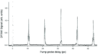
Figure 2: Recorded DFWM signal (dots) as a function of pump-probe time delay in a static cell of CO₂ at room temperature for parallel polarizations. Pressure is 0.1 bar and the peak intensity of each pump is 19 TW/cm². Simulated signal [full line, Eq. (7)] is calculated at 20 TW/cm².

At higher intensity, a strong background is observed which heterodynes and distorts the alignment signal. This phenomenon is attributed to the contribution of a refractive index grating due to a spatial distribution of electron density. Indeed, the electronic density produced by ionization follows the spatial intensity distribution of the pump with a lifetime of several nanoseconds Siders . As a consequence, the refractive index seen by the probe is modified and a grating is formed. The effect becomes very strong as the peak intensity of the bright fringes approaches the ionization saturation intensity (200 TW/cm² for CO₂). Some applications of this effect, which limits the range of intensity for the present study of alignment, is discussed in Ref. Loriot .

IV.2 Perpendicular polarizations

To overcome the intensity limitation discussed above, the polarizations of the two pump beams have been crossed. In that case, no optical interferences occur, and the intensity is constant over the interaction volume, except for the overall Gaussian distribution. A polarization grating is formed as discussed in the previous sections. Nevertheless, the instantaneous total intensity for the linear polarization is twice that of the circular one. As the ionization process is a function of the instantaneous intensity, the ionization rate and the electron density reflect the periodic distribution of this quantity. A refractive index grating due to the electrons is formed as in the linear case. But as the ionization rate is the same for the two linear (along the $x$ and $y$-axis) and for the two circular polarizations (left and right), the grating has a periodicity twice that of the parallel polarizations case (A). The angle of diffraction is doubled and the probe diffracted by this grating can be spatially resolved from the one diffracted by the alignment-induced grating. The experiment is therefore not sensitive to the electron density grating.

The Hamiltonian describing the interaction of the molecules with an elliptic electric field as well as the induced dipole moment have been given in the theoretical section. It has been shown that the observed signal can be approximated by using the dipole moment (11) at low and moderate intensities. To simulate the experimental data, we thus used the same routine as for parallel polarizations. Some results are shown in Fig. 3. Again the transverse spatial profile of the pump pulses should be taken into account through a factor 1/2, i.e. the simulated intensity has to be compared to 1/2 times the maximum intensity of one pump beam. The degree of alignment, quantified by $\langle\cos^{2}\theta\rangle_{t}$, is directly deduced from simulations. Even though the higher experimental intensities correspond to saturation of $\langle\cos^{2}\theta\rangle_{r,t}-1/3$, the calculated intensity approaches the expected value (see Fig.3). The volume averaging of the signal tends to smooth out the saturation process of alignment. For much higher intensities, discrepancies between calculated and experimental ($I_{0}/2$) intensity should appear, as shown in Ref.RenardPRA2004 . This effect is due to the strong saturation of alignment at the center of the pumped volume. In that case, Eq.(11) can not be used and the observed signal is no more accurately simulated by Eq.(20). Nevertheless, it would be possible, even though it would be time consuming, to reproduce the experimental data by numerical simulation of Eqs.(9, 10).

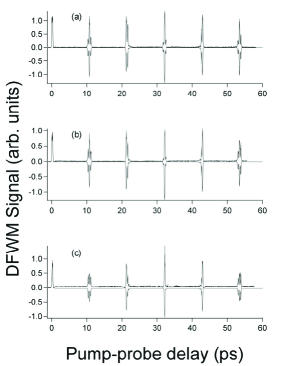
Figure 3: Experimental DFWM signal recorded as a function of the pump-probe time delay in CO₂ at room temperature for perpendicular polarizations. The pressure is 0.03 bar and pump peak intensity is (a) 37 TW/cm², (b) 78 TW/cm², and (c) 135 TW/cm². The numerical simulations [Eq. (7)] are shown inverted for (a) 15 TW/cm², (b) 30 TW/cm², (c) and 55 TW/cm². These theoretical values compare well with $I_{0}$/2 (see text).

One of the goals of the present work was to align cold molecules in order to increase the efficiency of the process. To obtain low temperatures, we used a pulsed supersonic jet in which the pressure is only a few mbar, depending on the distance from the nozzle. Before attempting an experiment, some preliminary studies at low static pressure and room temperature have been performed. The sensitivity was high enough to record signals at a pressure around 6 mbar of CO₂, with an excellent signal to noise ratio. The supersonic jet has allowed us to decrease the temperature down to 30 K (Fig. 4). The alignment that can be achieved at this temperature with an experimental intensity of 47 TW/cm² corresponds to $\langle\cos^{2}\theta\rangle=0.65$. This value is comparable to the one achieved at higher intensity in our previous study using a polarization technique at 60 K. But in the present case the experiment is free from heterodyne contribution due to spurious birefringence from optics.

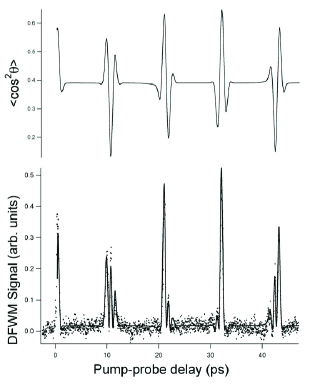
Figure 4: Recorded DFWM signal (lower panel, dots) as a function of pump-probe time delay in CO₂ at 30 K in the supersonic jet for perpendicular polarizations. Measured peak intensity of one pump is 47 TW/cm². Simulated signal [lower panel, full line, Eq. (7)] is calculated at 25 TW/cm². The calculated time dependence of $\langle\cos^{2}\theta\rangle$ is shown in the upper panel.

The polarization grating (case B) can be discussed in terms of alignment distribution, as for the intensity grating (case A). For example at a delay close to zero (modulo $T_{R}$), the molecules are aligned along the linear polarized field ($x$ and $y$-axis) and delocalized in the plane of polarization $xy$ (circular right and left). At time delay $T_{R}/4$ (modulo $T_{R}$), the molecules are delocalized in the planes $xOz$ or $yOz$, or aligned along the $z$-axis (circular right and left). Intermediate elliptic polarization leads to intermediate state of alignment.

V Conclusion

The main conclusions of this work are the following. DFWM experiments with two synchronized spatially crossed femtosecond pulses allow to produce transient gratings reflecting alignment of molecules. A contribution due to ionization and plasma formation appears at high intensities that heterodynes and therefore disturbs the experimental signal. With perpendicular polarizations, the alignment signal can be isolated from the plasma contribution. The experiments can thus be performed at higher intensity keeping a good signal to noise ratio. DFWM experiments prove to be very sensitive for probing low density and low temperature samples such as those obtained with a supersonic jet. Furthermore, it is shown that quantitative measurements of alignment are obtained through simulations by using a simplified model, even in the case of perpendicular polarizations which was a priori non-trivial.

Using different polarization schemes would permit to create interesting patterns of aligned molecules that could be used as a large frequency bandwidth spatial modulator.

Appendix A Postpulse alignment for low and moderate intensities

We analyse in this appendix the dependence of the postpulse alignment of linear molecules on the pump field intensities below the intrinsic saturation regime. We show in particular that (i) for a linearly polarized pulse the baseline of $\langle\cos^{2}\theta\rangle$ obeys the following law: quadratic and next linear, (ii) its shape is linear and (iii) the alignment induced by an elliptically polarized field can be analyzed in term of the decomposition into linearly polarized fields.

A.1 Linearly polarized field

A linearly polarized field leads to a postpulse alignment characterized by $\langle\cos^{2}\theta\rangle_{t}$, with $\theta$ the angle between the molecular axis and the field polarization axis, which can be generally characterized by

$$\langle\cos^{2}\theta\rangle_{t}-1/3=C+\sum_{J}|a_{J}|\cos(\omega_{J}t+\phi_{J}),$$ (12)

where $C$ is a constant value corresponding to the permanent alignment, and the second term, describing the rotational wave packet revivals, is written in terms of Fourier components of the amplitude $|a_{J}|$, the phase $\phi_{J}$, and the frequency $\omega_{J}$ (Raman frequency of rotational transitions). In the present experimental conditions, the phases are roughly constant: $\phi_{J}\approx-\pi/2$ RenardPRA2005 . Within the sudden impulsive regime (i.e. for $\tau\ll h/B$ with $\tau$ the duration of the pulse and $B$ the rotational constant of the molecule in Joule), where the pulse can be considered as a $\delta$-function, the coefficients $C$ and $|a_{J}|$ depend on the effective area

$$\xi=\Delta\alpha/4\hbar\int dt{E}^{2},$$ (13)

which is proportional to the peak field intensity $I$. For CO₂ molecules interacting with a Gaussian pulse of a full-width at half maximum $\tau_{\text{FWHM}}=0.1$ ps, we have $\xi\approx 0.444\times I[\text{TW/cm${}^{2}$}]$.

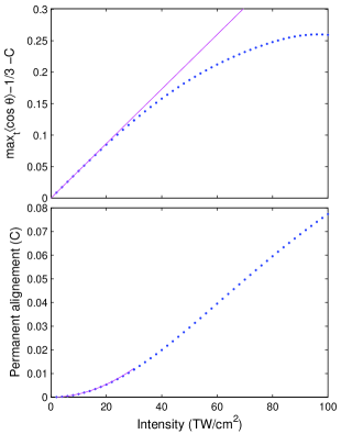
Figure 5: Permanent alignment $C$ and $\max_{t}\langle\cos^{2}\theta\rangle_{t}-1/3-C$ as a function of the peak pump intensity of $\tau_{\text{FWHM}}=0.1$ ps in CO₂ at $T=293$ K (dotted lines). The former is quadratic (full fitting line) approximately up to $I=30$ TW/cm² and linear for higher intensities. The latter is linear (full fitting line) for moderate intensities. Similar dependencies can be found for other linear molecules and temperatures.

Figure 5 shows the dependence of the law (12) on the pump intensity (centrifugal distorsion has not been considered in this study.) This allows us to define three regimes of intensity: (i) low intensity associated to a quadratic dependence of $C$ (here up to $I=30$ TW/cm²), (ii) moderate intensity associated to a linear dependence of $C$, and (iii) high intensity associated to the saturation of $\max_{t}\langle\cos^{2}\theta\rangle-1/3-C$. Below the saturation, one can consider with a good approximation that $\max_{t}\langle\cos^{2}\theta\rangle-1/3-C$ is approximately linear with the field intensity. This leads for low intensities to

$$\langle\cos^{2}\theta\rangle_{t}-1/3\approx\beta\xi^{2}+\kappa\xi f(t)\approx\kappa\xi f(t),$$ (14)

where, for a given molecule and temperature, $\kappa$ and $\beta$ are constant and $f(t)$ is a specific function independent of $\xi$. We can notice that the regime of low intensities extends the result of the perturbative regime, even if it is not itself a perturbative regime (usually defined as a small population transfer), since it can exhibit a non negligible alignment ($\max_{t}\langle\cos^{2}\theta\rangle_{t}\approx 0.45$ for $I=30$ TW/cm²). We also have $\beta\xi^{2}\ll\kappa\xi$, which shows that the permanent alignment is negligible for low intensities. For moderate intensity, Fig. 5 shows that the permanent alignment is linear with respect to the peak field intensity, which leads to

$$\langle\cos^{2}\theta\rangle_{t}-1/3\approx[\delta+\kappa f(t)]\xi.$$ (15)

We can thus conclude that at low and moderate intensities (i.e. below the saturation of alignment), $\langle\cos^{2}\theta\rangle_{t}-1/3$ is approximately proportional to $\xi$, i.e. to the pump intensity $I$.

A.2 Elliptically polarized field

We consider here the postpulse alignment induced by an elliptically polarized field $\vec{E}(t)={E}(t)(A\cos(\omega t)\vec{e_{x}}+B\sin(\omega t)\vec{e_{y}})$, $A^{2}+B^{2}=1$. The associated interaction reads

$$H_{\text{int}} = -\frac{\Delta\alpha}{4}{E}^{2}(t)\left[\left(A^{2}-B^{2}\right)\cos^{2}\theta_{x}-B^{2}\cos^{2}\theta_{z}\right]\qquad$$ (16a)

$$= -\frac{\Delta\alpha}{4}{E}^{2}(t)\left[A^{2}\cos^{2}\theta_{x}+B^{2}\cos^{2}\theta_{y}\right]$$ (16b)

with the particular cases of linear polarizations along $x$ for $A=1$, along $y$ for $B=1$, and of circular polarization in the $(x,y)$ plane for $A=B=1/\sqrt{2}$.

In the sudden impulsive regime, the propagator reads (the pulse interacting with the molecule at time $t=0$)

$$U(t,0)=e^{-iJ^{2}Bt/\hbar}e^{i\xi A^{2}\cos^{2}\theta_{x}}e^{i\xi B^{2}\cos^{2}\theta_{y}},$$ (17)

where the irrelevant global phases have been omitted. This propagator can be interpreted as the propagator associated to two interactions with fields linearly polarized along $x$ of effective area $\xi A^{2}$ and along $y$ of effective area $\xi B^{2}$. To calculate the expectation value (10), we first consider ($\langle\cos^{2}\theta_{i}\rangle_{t}-1/3$) ($i=x,y,z$) as a superposition of two quantities corresponding to the action of the two fields :

$$\langle\cos^{2}\theta_{i}\rangle_{t}-1/3 = (\langle\cos^{2}\theta_{i}\rangle_{t}-1/3)_{x-polar,A^{2}}$$

$$+(\langle\cos^{2}\theta_{i}\rangle_{t}-1/3)_{y-polar,B^{2}},$$

where the first term is calculated for the $x-$polarized field with a weighting factor $A^{2}$ and the second one for the $y-$polarized field with a weighting factor $B^{2}$. Beginning with $i=x$, the first term as estimated from (15), is $\approx A^{2}\xi(\delta+\kappa f(t))$. For the $y-$polarized field, we would have by symmetry $\langle\cos^{2}\theta_{x}\rangle_{t}=\langle\cos^{2}\theta_{z}\rangle_{t}$, and thus $\langle\cos^{2}\theta_{x}\rangle_{t}=(1-\langle\cos^{2}\theta_{y}\rangle_{t})/2$, using the property $\cos^{2}\theta_{x}+\cos^{2}\theta_{y}+\cos^{2}\theta_{z}=1$. The second term is therefore $\approx-\frac{1}{2}B^{2}\xi(\delta+\kappa f(t))$, using again 15. The summation in (A.2) gives $\langle\cos^{2}\theta_{x}\rangle_{t}-1/3\approx\xi(A^{2}-B^{2}/2)(\delta+\kappa f(t))$. Performing the same calculation for $i=y,z$, we finally find that in the intermediate field regime,

$$\langle\cos^{2}\theta_{x}\rangle_{t}-1/3 \approx \xi(A^{2}-B^{2}/2)(\delta+\kappa f(t)),\qquad$$ (19a)

$$\langle\cos^{2}\theta_{y}\rangle_{t}-1/3 \approx \xi(B^{2}-A^{2}/2)(\delta+\kappa f(t)),\qquad$$ (19b)

$$\langle\cos^{2}\theta_{z}\rangle_{t}-1/3 \approx -\xi(\delta+\kappa f(t))/2.\qquad$$ (19c)

We have in particular that $\langle\cos^{2}\theta_{x}\rangle_{t}-1/3$ is well approximated by the quantity $\xi(\delta+\kappa f(t))$ obtained from the interaction with a linearly polarized field of peak intensity $I$ times the scale factor $(A^{2}-B^{2}/2)$. We remark that $\langle\cos^{2}\theta_{z}\rangle_{t}-1/3$ does not depend on the ellipticity. We also notice that $\langle\cos^{2}\theta_{y}\rangle_{t}-1/3\approx 0$ when $B^{2}=A^{2}/2$, i.e. $B^{2}=1/3,A^{2}=2/3$. This particular ellipticity allows the directions $\theta_{x}$ and $\theta_{z}$ to play a symmetric role in (16a). This property has been used in Ref. Daems to demonstrate the optimal alternation of postpulse alignment.

For perpendicular polarizations, the observable $\langle\cos^{2}\theta_{x}\rangle_{t}-\langle\cos^{2}\theta_{y}\rangle_{t}$ is required. We obtain

$$\langle\cos^{2}\theta_{x}\rangle_{t}-\langle\cos^{2}\theta_{y}\rangle_{t}\approx\frac{3}{2}(A^{2}-B^{2})\xi(\delta+\kappa f(t))$$ (20)

We can conclude that a good approximation for $\langle\cos^{2}\theta_{x}\rangle_{t}-\langle\cos^{2}\theta_{y}\rangle_{t}$ can be obtained in the intermediate regime by calculating numerically $\langle\cos^{2}\theta_{i}\rangle_{t}-1/3$ with a single field linearly polarized along $i$ of intensity $I$ and by applying the scale factor $\frac{3}{2}(A^{2}-B^{2})$.