Teaching the Environment to Control Quantum Systems

Abstract

A non-equilibrium, generally time-dependent, environment whose form is deduced by optimal learning control is shown to provide a means for incoherent manipulation of quantum systems. Incoherent control by the environment (ICE) can serve to steer a system from an initial state to a target state, either mixed or in some cases pure, by exploiting dissipative dynamics. Implementing ICE with either incoherent radiation or a gas as the control is explicitly considered, and the environmental control is characterized by its distribution function. Simulated learning control experiments are performed with simple illustrations to find the shape of the optimal non-equilibrium distribution function that best affects the posed dynamical objectives.

I Introduction

The manipulation of coherent atomic and molecular dynamics often utilizes shaped electromagnetic fields as the control. This topic is the focus of extensive theoretical and experimental research R0 ; R1 ; R2 ; R3 ; R4 ; R5 ; R6 which relies on tailoring constructive and destructive interferences between different dynamical pathways of a quantum system. Many laboratory implementations of quantum control with lasers use adaptive feedback learning techniques JR .

In the present paper we consider the manipulation of atomic and molecular dynamics with the control being a tailored non-equilibrium, and generally time-dependent, state of the surrounding environment. Different non-equilibrium states of the environment can induce correspondingly unique dynamical responses in the physical system being controlled. Incoherent control by the environment (ICE) is distinct from operations with coherent control. Control by ICE affects a system through dissipative dynamics and can be used to steer the system from a pure or a mixed state into mixed and in some cases pure states. Control by lasers normally affects the system through Hamiltonian evolution and transforms pure states into the pure states. In practice limitations will exist on laser controls and the capabilities of ICE as well. Thus, in the most general circumstance a shaped laser pulse and a tailored non-equilibrium environment could be combined into an overall tool to simultaneously best perform control by Hamiltonian and dissipative dynamics.

This paper explicitly considers ICE implemented by two types of environments: incoherent radiation (i.e., a gas of photons) and gas of particles (i.e., electrons, atoms, or molecules). The particles of an environment (i.e., photons or matter) are characterized by their momenta ${\bf k}$ and internal degrees of freedom indexed by $\alpha$. For photons $\alpha$ denotes polarization while for atoms or molecules it denotes their internal energy levels. The environment is described by the distribution of mean occupation numbers $n_{{\bf k},\alpha}(t)$ of its microscopic states $|{\bf k},\alpha\rangle$ at time $t$. Thermal equilibrium states are characterized by only a few parameters, such as temperature and chemical potential, which uniquely determine the corresponding equilibrium distribution. Non-equilibrium states are characterized by occupation numbers of all microscopic states and have much richer structure. The control considered with ICE is the generally time dependent distribution function $n_{{\bf k},\alpha}(t)$. The shape of this function (i.e., its dependence on ${\bf k}$, $\alpha$, and $t$) together with the interaction Hamiltonian determines the dynamics of the system under control. Although operation with ICE does not induce coherent dynamics, nevertheless the shaping of $n_{{\bf k},\alpha}(t)$ over ${\bf k},\alpha$, and $t$ provides considerable flexibility for system manipulation. Many control objectives can be expressed in terms of creating specific mixed states of a system, which should be amenable to utilizing non-equilibrium environmental states for their preparation. Certain pure states can also be reached with ICE. For example, incoherent radiation can steer a three-level $\Lambda$-atom from the ground state to the intermediate excited state, a gas can steer a two-level atom through collisions to the excited state, etc.

The practical creation of controls for implementing ICE is important to consider. First, incoherent non-equilibrium radiation as a control includes monochromatic incoherent light, thermal radiation propagating in a medium with frequency sensitive absorbtion (i.e., filters), and radiation from luminescent emission. In the simplest case monochromatic radiation can be either coherent or incoherent, and in both circumstances it is composed of waves with the same wavelength. In the second formulation of ICE, a non-equilibrium gas, or more generally a surrounding fluid or solid medium, of particles is described by its distribution over momenta and internal degrees of freedom (e.g., vibrational and rotational modes of molecules or atomic energy levels). A non-equilibrium state of a gas may be generated in a number of ways, including through a sudden change in its thermodynamic parameters. For example, if a lower energy level of a molecule relaxes to equilibrium faster than an upper level, then a sudden temperature drop can create a non-equilibrium state with population inversion. A non-equilibrium particle momentum distribution can be created using selective excitation of the internal degrees of freedom by a laser with subsequent collisional transfer of the excitations into momentum modes. Lasers can have dual roles in this general circumstance of (a) directly addressing the system Hamiltonian for control as well as (b) first addressing the environment for its subsequent controlled manipulation of the system.

The main impediments to designing coherent optimal control fields are the required detailed knowledge of the system Hamiltonian and the need to solve the generally high dimensional Schrödinger equation. The difficulties in handling these two issues inevitably lead to significant errors in the field designs which would likely result in ineffective control in laboratory experiments. To overcome these difficulties optimal learning control in the laboratory is proving to be very successful JR . In this fashion the system subjected to control is used as an analog computer which solves its own Schrödinger equation exactly in real time and with the true laser field and system Hamiltonian. The capabilities of high duty cycle laser pulse shaping along with fast observation of the controlled outcome allows for efficient pattern recognition algorithms (e.g., genetic algorithms GA ) to guide a sequence of experiments to home in on the specified system control objective. The same logic is proposed for ICE to find an optimal non-equilibrium environment as a control, either alone or possibly in conjunction with determining a coherent control field.

This paper considers the following control problem: for a given target state of the system $\rho^{\rm T}$, find a distribution function of the environment $n_{{\bf k},\alpha}(t)$ such that the corresponding induced non-unitary system dynamics is steered from some initial state $\rho_{\rm I}$ as close as possible to the state $\rho^{\rm T}$. The corresponding objective function can be chosen as $J[n_{{\bf k},\alpha}(t)]=[\sum_{nm}(\rho_{nm}-\rho_{nm}^{\rm T})^{2}]^{1/2}$, where $\rho_{nm}$ is an element of the density matrix $\rho=\rho(t_{f})$ at some final time $t_{f}$ evolved from $\rho_{\rm I}$ under the action of the environment with distribution function $n_{{\bf k},\alpha}(t)$. The problem of creating an effective control based on significant environmental interactions generally requires an adaptive learning control procedure. The advantage of learning control lies in its ability to find an optimal distribution $n_{{\bf k},\alpha}(t)$ even if the details of the system, environment and their interactions are not known. In the laboratory, practical feedback signals would be of the form ${\rm Tr}\,\rho\Theta$, where $\Theta$ is an observable operator, and the goal would be to steer ${\rm Tr}\,\rho\Theta$ towards the desired value ${\rm Tr}\,\rho^{\rm T}\Theta$. In the more general case, expectation values of several possibly noncommutative observable operators $\Theta_{i}$ could be used for feedback, and the goal would be to steer the expectation value of each $\Theta_{i}$ towards its desired value. Other observable properties of the system, the environment, or the means of generating its non-equilibrium state also can be incorporated into the objective function.

Learning control driven by a GA is employed in the present paper in simulations of the potential effectiveness of ICE using either incoherent radiation or a gas as controls. In these cases there is a Markovian regime (i.e., weak coupling and low density) for the reduced dynamics of the controlled system SL ; Sp ; ldl ; apv . Master equations with appropriate dissipative terms are reasonable models in this regime. These equations are used here to simulate evolution of the system’s density matrix towards the target under the influence of a non-equilibrium environment. The general ICE concept is not limited to the models used here, and in the laboratory fully non-Markovian dynamics naturally would be included as required.

An environment prepared impulsively in a non-equilibrium state will evolve to equilibrium. In the simulations below we consider control by stationary non-equilibrium environments. In practice this requires keeping the environment in a non-equilibrium state for a time which is sufficiently long to perform the control. In the simulations the master equations will be followed temporally until a steady state is reached for the control outcome. A stationary non-equilibrium state for incoherent radiation can easily be maintained using steady sources. In addition, a non-equilibrium state of a stationary gas can be maintained by controlling the gas with a suitable external field. An example of such control is preparation of population inversion in the He–Ne gas-discharge laser. In this case we may consider the gas of He atoms as the control environment and the Ne atoms as the controlled system. An electric discharge is passed through the He–Ne gas to bring the He atoms into a non-equilibrium state. Then He–Ne collisions transfer the energy of the non-equilibrium state of the He atoms into the high energy levels of the Ne atoms. This process creates a population inversion in the Ne atoms and subsequent lasing. A steady electric discharge can be used to keep the gas of helium atoms in a non-equilibrium state to produce a CW He–Ne laser. In the present simulations the actual nature of the external control creating the non-equilibrium steady distribution $n_{\bf k}$ will not be explicitly described. Rather in keeping with exploring the ICE concept, $n_{\bf k}$ will be treated directly as the control for optimization as a function of ${\bf k}$. In the laboratory the external control settings would be guided by the learning algorithm using the system observations as a feedback signal.

Control by several lasers with incoherent relative phases was considered in cbs . In this approach the interference between different channels is manipulated by changing the relative frequencies and intensities of the lasers. Although the relative phases between the lasers are incoherent, each of the lasers is a source of coherent radiation which affects the system through induced Hamiltonian dynamics. The present paper, in its part devoted to control by radiation, uses as the control totally incoherent radiation which affects the system through induced dissipative evolution.

There is a relation between ICE and recently proposed measurement-assisted GR and dual material-photonic reagent control MPC . In all these situations control is implemented, at least partially, through induced dissipative dynamics. The ICE proposal directly exploits the influence of an optimally shaped environmental distribution function upon the dynamics of the controlled system. Measurement-assisted control exploits the back action of decoherence induced by measurements. Material-photonic reagent control utilizes dynamics driven by a laser as well as identification of an optimal material for the system and/or the environment. All these approaches to molecular or condensed phase system manipulation can be considered as different branches of the general perspective of introducing control through same aspects of dissipative dynamics.

Sections II and III present simple illustrations of ICE using incoherent radiation and a gaseous medium, respectively. The formulations will be developed in the general context of a coherent field being present for directly addressing the system along with a time-dependent environmental control distribution function $n_{\bf k}(t)$. The test simulations will be performed with steady distributions and without a coherent control field to serve as a simple demonstration of the basic closed-loop ICE concept. Even richer control should be possible with temporal control densities operating along with a coherent field $\varepsilon(t)$. Brief concluding remarks are given in Section IV.

II Incoherent radiation serving as a control

This section considers control by non-equilibrium incoherent radiation described by a distribution $n_{\bf k}$ of the photon momenta. In general, the polarization dependence of the incoherent radiation also can be exploited as an additional control along with the propagation direction in cases where spatial anisotropy is important (e.g., a system consisting of oriented molecules bound to a surface).

The thermal (i.e., equilibrium) distribution of photons at temperature $T$ and frequency $\omega$ is determined by Planck’s formula $N_{\omega}=\omega^{2}/\pi^{2}c^{3}[\exp\left(\hbar\omega/k_{\rm B}T\right)-1]$, where $c$ is the speed of light, $k_{\rm B}$ and $\hbar$ are the Boltzmann and the Planck constants (we set them to $1$ in the sequel). Non-equilibrium incoherent radiation may have an arbitrary distribution. Fig. 1 gives an example of a thermal distribution and a non-equilibrium distribution, which corresponds to incoherent radiation composed of three nearly monochromatic components of differing intensity. The latter distribution may be produced either by filtering the thermal radiation or by using independent monochromatic sources.

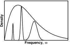
Figure 1: The Planck density of black body radiation (upper curve) and the density (un-normalized) of non-equilibrium radiation composed of three nearly monochromatic sources (lower curve).

The master equation for a system simultaneously interacting with a coherent electromagnetic field $\varepsilon(t)$ and an environment with distribution $n_{\bf k}(t)$ generally has the form:

$$\frac{d\rho(t)}{dt}=-i[H_{0}+H_{\rm eff}-\mu\varepsilon(t),\rho(t)]+{\cal L}_{\rm diss}[n_{\bf k}(t);\rho(t)].$$ (1)

The coherent dynamics is generated by the system Hamiltonian $H_{0}=\sum_{n}\varepsilon_{n}P_{n}$ with eigenvalues $\varepsilon_{n}$ and the corresponding projectors $P_{n}$, the effective Hamiltonian $H_{\rm eff}$ originating from system-environment interaction, dipole moment $\mu$, and electromagnetic field $\varepsilon(t)$. The effective Hamiltonian commutes with $H_{0}$ and is not used in the following simulations.

The dissipative dynamics generated by the incoherent radiation distribution function $n_{{\bf k}}(t)$ has the form ${\cal L}_{\rm diss}[n_{\bf k}(t);\rho]={\cal L}^{{}^{\rm Rad}}_{\rm diss}[n_{\bf k}(t);\rho]=\sum\limits_{\omega}[\gamma^{+}_{\omega}(t)+\gamma^{-}_{-\omega}(t)](2\mu_{\omega}\rho\mu^{+}_{\omega}-\mu^{+}_{\omega}\mu_{\omega}\rho-\rho\mu^{+}_{\omega}\mu_{\omega})$ where the sum is taken over all system transition frequencies. Here the coefficients $\gamma^{\pm}_{\omega}(t)=\pi\int d{\bf k}\delta(|{\bf k}|-\omega)|g({\bf k})|^{2}[n_{\bf k}(t)+(1\pm 1)/2]$ determine the transition rates between energy levels with transition frequency $\omega$ and $\mu_{\omega}=\sum\limits_{\varepsilon_{n}-\varepsilon_{m}=\omega}P_{m}\mu P_{n}$. The transition rates are the functions of the photon density $n_{\bf k}(t)$ and matrix elements of the dipole moment $\mu$. The form-factor $g({\bf k})$ determines the coupling of the system to the ${\bf k}$-th mode of the field. If for all ${\bf k}$, $n_{\bf k}\equiv 0$, (i.e., the quantum system is in a vacuum), then $\gamma^{-}_{\omega}\equiv 0$, and the coefficients $\gamma^{+}_{\omega}$ together with dipole moment $\mu$ determine the inverse lifetime of the system’s energy levels. The positivity of $\gamma^{\pm}_{\omega}(t)$ guarantees that the off-diagonal elements of the density matrix vanish at sufficiently long time.

As a specific example, numerical simulations are performed for control of a four-level system by means of incoherent radiation with the distribution $n_{k}$ in terms of the magnitude of the photon momenta $k\equiv|{\bf k}|$; no direct coherent control is present such that $\varepsilon(t)=0$. The system has the free Hamiltonian $H_{0}={\rm diag}\{0;\,11;\,13;\,24\}$ and dipole moment matrix

$$\mu=\left(\begin{array}[]{c c c c}0&0.8&0.3&0.5\\ 0.8&0&0.2&0.7\\ 0.3&0.2&0&1\\ 0.5&0.7&1&0\end{array}\right)$$ (2)

All transitions amongst the energy levels are allowed, and the system is assumed to initially be in its ground state. The goal of the control effort is to steer the system to a target mixed state $\rho^{\rm T}$ (we consider several examples for $\rho^{\rm T}$). The corresponding objective function is chosen to have the form $J[n_{k}]=[\sum_{nm}(\rho_{nm}-\rho^{\rm T}_{nm})^{2}]^{1/2}$ where $\rho_{nm}$ and $\rho^{\rm T}_{nm}$ are elements of the system’s density matrix and the target density matrix, respectively. The goal is to minimize the objective function at a sufficiently long time such that $\rho$ is stationary.

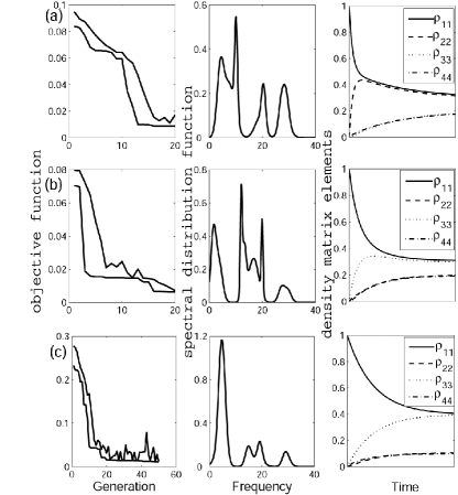
Figure 2: Results of ICE simulations with tailored incoherent radiation as the control for target states (a) $\rho^{\rm T}={\rm diag}(0.3;\,0.3;\,0.2;\,0.2)$, (b) $\rho^{\rm T}={\rm diag}(0.3;\,0.2;\,0.3;\,0.2)$, and (c) $\rho^{\rm T}={\rm diag}(0.4;\,0.1;\,0.4;\,0.1)$. Each case shows: the objective function vs GA generation, the optimal spectral distribution vs frequency, and the evolution of the diagonal matrix elements of the density matrix for the optimal distribution. In the plots for the objective function the upper curve is the average value for the objective function and the lower one is the best value in each generation.

Each distribution function $n_{\bf k}$ determines the quantum dynamical semigroup $P^{t}_{n_{\bf k}}=e^{t{\cal L}_{n_{\bf k}}}$, $t\geq 0$ with generator ${\cal L}_{n_{\bf k}}[\,\cdot\,]:=-i[H_{0},\cdot]+{\cal L}^{{}^{\rm Rad}}_{\rm diss}[n_{\bf k};\cdot]$. An invariant state of the semigroup $\rho_{\rm inv}$ is defined by ${\cal L}_{n_{\bf k}}[\rho_{\rm inv}]=0$ (thus $P^{t}_{n_{\bf k}}(\rho_{\rm inv})=\rho_{\rm inv}$). The solution of Eq. (1) with initial condition $\rho(t=0)=\rho_{0}$ has the form $\rho(t)=P^{t}_{n_{\bf k}}[\rho_{0}]$. If the coefficients $\gamma^{\pm}_{\omega}$ are nonzero then the system density matrix $\rho(t)$ will converge at long time to $\rho_{\rm inv}$. For a given distribution function $n_{\bf k}$ one can compute the corresponding Lindblad operator ${\cal L}_{n_{\bf k}}$ and find its invariant. Here we consider the inverse problem: given a target state $\rho^{\rm T}$ find a distribution function of the environment $n_{\bf k}$ which generates the Lindblad operator ${\cal L}_{n_{\bf k}}$ whose invariant state is as close as possible to $\rho^{\rm T}$. In the case of control by radiation only values of $n_{\bf k}$ at the system transition frequencies generally have an effect on the dynamics. In principle, these values of $n_{\bf k}$ could be calculated if there was full knowledge of the system, environment and their interaction. This circumstance is rarely the case, and for a gaseous medium the situation is even more complex, since generally all modes of the gas contribute to the dynamics [see Eq. (3)]. Even with all of these uncertain conditions learning control can be effective because it only relies on laboratory control-response observations.

The non-equilibrium radiation distribution function is modelled as $n_{k}=\exp(-\beta k)\sum_{i=1}^{10}\exp[-(k-k_{i})^{2}/2D_{i}]/\sqrt{2\pi D_{i}}$ with $\beta=1/20$. The parameters $D_{i}$ and $k_{i}$ are optimized over ranges large enough to include all of the system transition frequencies. A set of these parameters forms an individual in the population for the GA to operate with. Each individual determines a distribution function $n_{k}$ which is used to drive the evolution of the system density matrix $\rho(t)$ towards its stationary form as $t\to\infty$ to ultimately determine the objective function. In practice, the time $t$ only needs to be taken out to some small multiple of the longest timescale of the system transitions.

A GA with crossover and mutation operators is used to find the optimal values for $k_{i}$ and $D_{i}$. The number of individuals in each population is $14$. The total of $20$ variables form an individual corresponding to ten parameters $k_{i}$ and $D_{i}$. Each variable is coded into a string of $20$ bits. The two most fit individuals are always retained in the successive generation. The remaining twelve individuals are produced from the parent population using the crossover and mutation operators. The fitness function determines the number of times each individual from the parent generation is chosen to produce offsprings in the next generation. The probability of crossover is $P_{x}=0.9$ and of mutation (a bit flip) is $P_{m}=0.7/L_{\rm ind}$, where $L_{\rm ind}=400$ is the length of the bit string forming an individual.

The results of the simulations for three different target states are presented in Fig. 2. Each case contains plots of the objective function vs generation, the optimal spectral distribution function vs frequency, and the corresponding evolution of the system density matrix. In each case the target objective is met very well with a suitable spectral distribution function. The fitness function in cases (a) and (b) has small values for the initial population because most randomly chosen distribution functions $n_{k}$ induce states of the system which are close to the equally populated state. Hence, the search for a distribution function which steers the system to a complex target state is a non-trivial problem. A general expectation is that certain modes of radiation will promote transitions to the target state whereas others may be harmful for control. Thus, it is found that distinct distributions of radiation energy are required to most effectively steer the system into each particular target state. Each of the radiation distribution functions has components at all of the system transition frequencies, and the mechanism of the control is not simply evident in each case. Further analysis abhra would be needed to identify the control mechanism. In keeping with the logic of the adaptive control technique, the learning algorithm deduces how to distribute the radiation energy without specific knowledge or details of the microscopic dynamics, including the Hamiltonian and initial state of the system, as well as details of its coupling to the non-equilibrium environment. Fig. 2 shows that excellent results can be achieved even with diverse choices for the target density matrix.

Using incoherent radiation as the control clearly has some limitations. For example, incoherent radiation can not create population inversion in a two-level atom. However incoherent radiation can steer a quantum system from a pure state to a mixed one, possibly of a complex structure as indicated in Fig. 2, and in some cases specific pure states can also be reached. Tailored incoherent radiation also can be used jointly with a laser field $\varepsilon(t)$ to improve the degree of system control when significant laser restrictions exist, such as bounds on laser intensity or bandwidth.

III A gaseous medium serving as a control

This section considers ICE with a non-equilibrium density $n_{\bf k}(t)$ of gas particles such as electrons, atoms or molecules serving as the control. Quantum systems interacting with such gases are described by master equations whose dissipative generators are different from ${\cal L}^{{}^{\rm Rad}}_{\rm diss}$ in Section II. The gas is assumed to be sufficiently dilute such that the reduced dynamics of the system is Markovian. In this case the probability of simultaneous interaction of the system with two or more particles of the gas is negligible and the reduced dynamics is determined by two body scattering events between one particle of the system and one particle of the gas. The assumption of the rarity of the gas is not a restriction for ICE, and dense gases might be used for control as well.

The master equation for a system interacting with a coherent electromagnetic field $\varepsilon(t)$ and a gas has the form of Eq. (1) with the dissipative generator ${\cal L}_{\rm diss}[n_{\bf k}(t);\rho]={\cal L}^{{}^{\rm Gas}}_{\rm diss}[n_{\bf k}(t);\rho]$ specified by the distribution function of the gas $n_{\bf k}(t)$ and by the $T$-operator (transition matrix) for scattering of the system and a gas particle. A transition matrix element is $T_{n,n^{\prime}}({\bf k},{\bf k}^{\prime})=\langle n,{\bf k}|T|n^{\prime},{\bf k}^{\prime}\rangle$, where $|n,{\bf k}\rangle\equiv|n\rangle|{\bf k}\rangle$ denotes the product state of the system discrete eigenstate $|n\rangle$ (an eigenstate of the system’s free Hamiltonian $H_{0}$ with eigenvalue $\varepsilon_{n}$) and a translational state of the system and a gas particle with relative momentum ${\bf k}$. If the system is fixed in space (we consider this case below corresponding to the system particle being much more massive than the particles of the surrounding gas) then $|{\bf k}\rangle$ is a translation state of a gas particle. The general case of relative system gas particle motion can be considered as well using suitable master equations. We assume that the particles of the gas are characterized only by their momenta and do not have internal degrees of freedom; otherwise, the state of one particle of the gas should have the form $|{\bf k},\alpha\rangle$, where $\alpha$ specifies the state of the internal degrees of freedom. It is convenient to introduce the notation $T_{\omega}({\bf k},{\bf k}^{\prime}):=\sum\limits_{m,n:\,\,\varepsilon_{m}-\varepsilon_{n}=\omega}T_{m,n}({\bf k},{\bf k}^{\prime})|m\rangle\langle n|$. The density of particles of the gas at momentum ${\bf k}$ is $n_{\bf k}(t)$, the kinetic energy of a gas particle of mass $M$ is $|{\bf k}|^{2}/2M$, and $B$ is the set of transition frequencies $\omega$ of the system among the energy levels of $H_{0}$. In this notation the dissipation generator is

$${\mathcal{L}}^{{}^{\rm Gas}}_{\rm diss}[n_{\bf k}(t);\rho] = 2\pi\sum\limits_{\omega\in B}\int d{\bf k}d{\bf k}^{\prime}\delta\left(\frac{|{\bf k}^{\prime}|^{2}}{2M}-\frac{|{\bf k}|^{2}}{2M}+\omega\right)n_{\bf k}(t)\Bigl{[}T_{\omega}({\bf k}^{\prime},{\bf k})\rho T^{+}_{\omega}({\bf k}^{\prime},{\bf k})$$ (3)

$$-\frac{1}{2}\Bigl{(}T^{+}_{\omega}({\bf k}^{\prime},{\bf k})T_{\omega}({\bf k}^{\prime},{\bf k})\rho+\rho T^{+}_{\omega}({\bf k}^{\prime},{\bf k})T_{\omega}({\bf k}^{\prime},{\bf k})\Bigr{)}\Bigr{]}$$

If the gas is at equilibrium with inverse temperature $\beta$, then the density is stationary and has the Boltzmann form $n_{\bf k}(t)\equiv n_{\bf k}=C(\beta,n)\exp(-\beta|{\bf k}|^{2}/2M)$, where the normalization constant $C(\beta,n)$ is determined by the condition $\int d{\bf k}n_{\bf k}=n$, where $n$ is the total density of the gas. The structure of Eq. (3) for equilibrium gases has been discussed previously in ldl ; apv and for non-equilibrium stationary gases in p . Non-equilibrium gases may be characterized by generally time dependent distributions. Equation (1) with ${\cal L}_{\rm diss}[n_{\bf k}(t);\rho(t)]={\cal L}^{{}^{\rm Gas}}_{\rm diss}[n_{\bf k}(t);\rho(t)]$ is the general formulation for control by both a coherent electromagnetic field $\varepsilon(t)$ and a non-equilibrium gas density $n_{\bf k}(t)$. As a simple illustration of ICE we only consider a simulation for control by a static non-equilibrium distribution $n_{\bf k}$.

Let $E_{i,n}=|{\bf k}|^{2}/2M+\varepsilon_{n}$ be the initial energy of the total system consisting of one gas particle and the controlled system before collision and let $E_{f,m}=|{\bf k}^{\prime}|^{2}/2M+\varepsilon_{m}$ be the final energy after the collision. If for each transition frequency $\omega$ there are only two system levels $n$ and $m$ such that $\omega=\varepsilon_{n}-\varepsilon_{m}$, then Eq. (1) for the diagonal elements of the density matrix reduces to the Pauli master equation

$$\frac{d\rho_{ll}(t)}{dt}=2\sum\limits_{n}\bigl{[}w_{ln}\rho_{nn}(t)-w_{nl}\rho_{ll}(t)\bigr{]}$$

where the transition probability $w_{mn}=\pi\int d{\bf k}n_{\bf k}(t)\int d{\bf k}^{\prime}\delta(E_{f,m}-E_{i,n})|T_{mn}({\bf k}^{\prime},{\bf k})|^{2}$ between levels $n$ and $m$ is explicitly determined by the distribution function $n_{\bf k}(t)$.

The quantity $\int d{\bf k}^{\prime}\delta(E_{f,m}-E_{i,n})|T_{mn}({\bf k}^{\prime},{\bf k})|^{2}$ defines the scattering cross section between the system and one gas particle. There are two possible strategies for investigating the prospects for control by a non-equilibrium gas. First, one may start with the microscopic interaction Hamiltonian between the system and a particle of the gas to compute the $T$-matrix for use in the dissipative generator (3). The second strategy is to use experimentally measured cross sections for the same purpose. As our purpose here is to illustrate the prospect of closed-loop laboratory learning control with ICE, we will simply use the first option in a model.

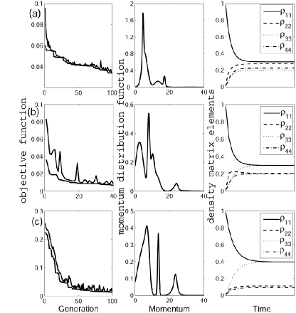
Figure 3: Results of ICE simulations with a surrounding non-equilibrium gas as the control for target states (a) $\rho^{\rm T}={\rm diag}(0.3;\,0.3;\,0.2;\,0.2)$, (b) $\rho^{\rm T}={\rm diag}(0.3;\,0.2;\,0.3;\,0.2)$, and (c) $\rho^{\rm T}={\rm diag}(0.4;\,0.1;\,0.4;\,0.1)$. Each case shows: the objective function vs GA generation, the optimal distribution vs momentum, and the evolution of the diagonal elements of the density matrix for the optimal distribution. In the plots for the objective function the upper curve is the average value for the objective function and the lower one is the best value in each generation.

In the simulations we consider a four-level system with the same free Hamiltonian $H_{0}$ in Section II, immersed in a dilute gas. The system is initially prepared in its ground state and the goal of the control is to steer the system to a target state $\rho^{\rm T}$ (we consider the same target states and the same fitness function as in Section II). The interaction $V$ between the system and one particle of the gas is considered to be weak with matrix elements $V_{nm}({\bf k},{\bf k}^{\prime})\equiv\langle n,{\bf k}|V|m,{\bf k}^{\prime}\rangle=\mu_{nm}g_{n}({\bf k})g_{m}({\bf k}^{\prime})$ defined by the matrix $\mu$ of the form (2) and by the functions $g_{n}({\bf k})$ chosen as characteristic functions of the momentum magnitude $k\equiv|{\bf k}|$, $g_{n}({\bf k})=\chi_{[a_{n},b_{n}]}(k)$. Here $\chi_{[a_{n},b_{n}]}(k)$ has unit value if $a_{n}\leq k\leq b_{n}$ and zero otherwise. The parameters $a_{n}$ and $b_{n}$ are chosen randomly as $a_{1}=2$, $b_{1}=12$, $a_{2}=9$, $b_{2}=24$, $a_{3}=3$, $b_{3}=17$, $a_{4}=14$, and $b_{4}=26$. We chose $M=1$.

The matrix $\mu$ describes transitions between the system’s energy levels due to interaction with the gas and the functions $g_{n}({\bf k})$ describe the corresponding change in the momentum of a gas particle. For a general $\mu$ its diagonal elements are responsible for elastic scattering of the system (these elements are zero in our case), whereas the off-diagonal ones control the inelastic events. Spontaneous emission from the upper levels is assumed to be negligible, corresponding to the lifetimes of the excited states being much longer than the inverse transition rates due to collisions with the gas. Elastic scattering and spontaneous emission can be included when necessary, and all physical processes could naturally be present in a laboratory closed loop experiment.

The weak nature of the interaction allows for replacing the $T$-operator in Eq. (3) by the interaction Hamiltonian $V$. The control in the simulations is a static distribution of the form $n_{k}=\exp(-\beta k^{2})\sum_{i=1}^{10}\exp[-(k-k_{i})^{2}/2D_{i}]/\sqrt{2\pi D_{i}}$ with $\beta=0.01$. The parameters $k_{i}$ and $D_{i}$ are optimally determined by the GA. This distribution together with interaction Hamiltonian determines the dissipative generator ${\cal L}_{\rm diss}^{{}^{\rm Gas}}$ according to Eq. (3) and the evolution of the system density matrix according to the master equation (1) (with $\varepsilon(t)=0$ in this case). The goal of the control is to find a stationary non-equilibrium state of the gas which steers the system to a target state $\rho^{\rm T}$. If desired, either the constraint of a fixed total energy of the gas or its cost for minimizing its value could be included by adding appropriate terms to the objective function. Fig. 3 gives the results of the numerical simulation for different target states. The simulations show that diverse mixed states can be reached very well by manipulating the momentum distribution function $n_{k}$ using ICE based on a learning algorithm.

IV Conclusions

In this paper learning control with a non-equilibrium environment is proposed as a means for manipulating quantum systems. Two cases are simulated: control by incoherent radiation and by a gas of particles. The control is the distribution of mean occupation numbers of the environment. The control affects the physical system through tailored dissipative dynamics and allows for steering an initial pure or a mixed state into a complex target state. The search for an optimal control distribution in ICE is performed by a learning control strategy, which could be implemented in the laboratory without detailed knowledge of the system Hamiltonian, coupling to the environment, etc. The method can be generalized by combining standard laser control and the proposed ICE control. In the latter case a most interesting situation would be attaining states which can not be obtained by using either restricted lasers or a non-equilibrium environment alone. An open issue is to establish the degree of control, i.e., the set of states reachable with ICE.

- (1) D. Tannor and S. A. Rice, J. Chem. Phys. 83, 5013 (1985).
- (2) P. Brumer and M. Shapiro, Chem. Phys. Lett. 126, 541 (1986).
- (3) W. S. Warren, H. Rabitz and M. Dahleh, Science 259, 1581 (1993).
- (4) H. Rabitz, R. de Vivie-Riedle, M. Motzkus and K. Kompa, Science 288, 824 (2000).
- (5) S. A. Rice and M. Zhao, Optical Control of Molecular Dynamics (Wiley: New York, 2000).
- (6) M. Shapiro and P. Brumer, Principles of the Quantum Control of Molecular Processes (Wiley-Interscience: Hoboken, NJ, 2003).
- (7) M. Dantus and V. V. Lozovoy, Chem. Rev. 104, 1813 (2004).
- (8) R. S. Judson and H. Rabitz, Phys. Rev. Lett. 68, 1500 (1992).
- (9) D. E. Goldberg, Genetic Algorithms in Search, Optimization and Machine Learning (Addison-Wesley, Reading, MA, 1989).
- (10) H. Spohn and J. L. Lebowitz, Adv. Chem. Phys. 38, 109 (1978).
- (11) H. Spohn, Rev. Mod. Phys. 53, 569 (1980).
- (12) R. Dümcke, Comm. Math. Phys. 97, 331 (1985).
- (13) L. Accardi, A. N. Pechen and I. V. Volovich, Infin. Dimens. Anal. Quant. Probab. and Relat. Topics 6, 431 (2003); E-print: math-ph/0206032.
- (14) Z. Chen, M. Shapiro and P. Brumer, Chem. Phys. Lett. 228, 289 (1994); Phys. Rev. A 52, 2225 (1995).
- (15) Gong J. and S. A. Rice, J. Chem. Phys. 120, 9984 (2004).
- (16) R. Wu, A. N. Pechen and H. Rabitz, in preparation.
- (17) A. Mitra and H. Rabitz, Phys. Rev. A 67, 033407 (2003).
- (18) A. N. Pechen, in QP-PQ: Quantum Probability and White Noise Analysis, Vol. 18, edited by M. Schürmann and U. Franz (World. Sci. Pub. Co., Singapore, 2005) pp. 428–447; E-print: quant-ph/0607134.