Quantum Walks in an array of Quantum Dots

Abstract

Quantum random walks are shown to have non-intuitive dynamics, which makes them an attractive area of study for devising quantum algorithms for well-known classical problems as well as those arising in the field of quantum computing. In this work we propose a novel scheme for the physical implementation of a discrete-time quantum random walk using laser excitations of the electronic states of an array of quantum dots. These dots represent the discrete nodes of the walk, while transitions between the energy levels inside each dot correspond to the required coin operation and stimulated Raman adiabatic passage (STIRAP) processes are employed to induce the steps of the walk. The quantum dot design is tailored in such a way as to enable selective coupling of the energy levels. Our simulation results show a close agreement with the ideal quantum walk distribution as well as modest robustness towards noise disturbance.

I Introduction

Quantum random walks represent a generalized version of the well known classical random walk, which can be elegantly described using quantum information processing terminology Aharonov et al. (1993). Despite their apparent connection however, dynamics of quantum random walks are often non-intuitive and deviate significantly from those of their classical counterparts Farhi and Gutmann (1998). Among the differences, the faster mixing and hitting times of quantum random walks are particularly noteworthy, making them an attractive area of study for devising efficient quantum algorithms, including those pertaining to connectivity and graph theory Kempe (2003); Farhi and Gutmann (1998); Childs et al. (2003), as well as quantum search algorithms Shenvi et al. (2003); Childs and Goldstone (2004).

There are two broad classes of quantum random walks, namely the discrete- and continuous-time quantum random walks, which have independently emerged out of the study of unrelated physical problems. Despite their fundamentally different quantum dynamics however, both families of walks share similar and characteristic propagation behavior Kempe (2003); Konno (2005); Patel et al. (2005). Strauch’s recent work Strauch (2006) is the latest in a line of theoretical efforts to establishing a formal connection between the discrete and continuous-time quantum random walks, in a manner similar to their classical counterparts.

There have been several proposals for implementing quantum random walks using a variety of physical systems including Nuclear Magnetic Resonance Du et al. (2003); Ryan et al. (2004), cavity QED Aharonov et al. (1993); Agarwal and Pathak (2005); Sanders and Bartlett (2003); Di et al. (2004), ion traps Travaglione and Milburn (2002), classical optics Zhi Zhao and Pan (2002); H. Jeong and Kim (2004); Do et al. (2005); Knight et al. (2003a, b); nuls et al. (2006); Francisco et al. (2006), quantum optics Zou et al. (2006); Zhang et al. (2007), optical multiports Hillery et al. (2003); Feldman and Hillery (2004); Košík and Bužek (2005), optical lattice and microtraps Dur et al. (2002); Chandrashekar (2006); Joo et al. (2006); Côté et al. (2006); Eckert et al. (2005) as well as quantum dots Solenov and Fedichkin (2006).

In this paper we introduce another proposal for implementing the discrete-time or coined quantum walk on a line using a series of stimulated Raman adiabatic passage (STIRAP) operations Bergmann et al. (1998); Král and Shapiro (2001); Hohenester et al. (2000) on a single electron trapped in an array of quantum dots. An important advantage of our proposal is that it relies on well established and generally accessible experimental techniques which result in both high fidelity operations as well as a relative ease of scalability. To the best of our knowledge, the proposal of Solenov and Fedichkin Solenov and Fedichkin (2006) is the only other implementation to date which employs quantum dots, but unlike our scheme, it pertains to a continuous-time quantum walk on a circle.

In what follows we present a brief overview of the coined quantum random walk (Sec. II) and describe our proposal for the design of the quantum dot array and the sequence of required STIRAP operations (Sec. III). We then present a numerical simulation of the system’s evolution (Sec. IV), including the effect of imperfect STIRAP operations. In the appendix we also demonstrate an efficient numerical technique for the optimization of STIRAP pulse parameters.

II Coined Quantum Random Walk

A one-dimensional quantum random walk consists of a walker hopping between $N$ nodes or quantum states $|i\rangle$ ($-N/2-1<i<N/2$) assembled in a line. In the coined quantum walk, each state $|i\rangle$ further consists of two sub-levels or coin states labeled as $|\uparrow,i\rangle$ and $|\downarrow,i\rangle$. Unlike the classical case, the quantum walker has a complex valued distribution $\psi$ over all the states, which remains undetected throughout the walk. Each step of the walk involves a coin flip, defined as a simultaneous unitary rotation

$$\hat{C}(\theta,\phi_{1},\phi_{2})=\left(\begin{array}[]{cc}\cos(\theta)&\sin(\theta)e^{i\phi_{1}}\\ \sin(\theta)e^{i\phi_{2}}&-\cos(\theta)e^{i(\phi_{1}+\phi_{2})}\end{array}\right),$$ (1)

on the coin states of all nodes, followed by a conditional translation which shifts the walker in states $|\uparrow,i\rangle$ and $|\downarrow,i\rangle$ to states $|\uparrow,i+1\rangle$ and $|\downarrow,i-1\rangle$ respectively. Hence for a quantum walker in an initial state $\psi(0)$, its state after $n$ steps of the walk is given by $\psi(n)=\hat{U}^{n}~{}\psi(0)$, where

$$\hat{U}=\hat{T}^{\downarrow}_{-1}~{}\hat{T}^{\uparrow}_{+1}~{}\hat{C}$$ (2)

is the overall evolution operator for a single step. A final probability distribution is determined by collapsing the walker’s wavefunction $\psi(n)$ at the end of the evolution.

In this paper, we implement a modified evolution operator

$$\widetilde{U}=\hat{T}^{\uparrow}_{+1}~{}\hat{C}$$ (3)

which is the same as Eq. 2 up to a translation and relabeling of states. In other words we can define a mapping $\hat{M}:\widetilde{U}\longmapsto\hat{U}$ where $\hat{M}=\hat{T}_{-1}~{}\hat{L}$ first relabels all the nodes according to $\hat{L}:|i\rangle\longmapsto|2i\rangle$, followed by a translation $\hat{T}_{-1}$ of the entire wavefunction one node to the left, that is

$$\hat{M}~{}\widetilde{U} = \hat{T}_{-1}~{}\hat{L}~{}~{}\hat{T}^{\uparrow}_{+1}~{}\hat{C}$$ (4)

$$= \hat{T}_{-1}~{}~{}\hat{T}^{\uparrow}_{+2}~{}\hat{C}$$

$$= \hat{T}^{\downarrow}_{-1}~{}\hat{T}^{\uparrow}_{-1}~{}\hat{T}^{\uparrow}_{+2}~{}\hat{C}$$

$$= \hat{T}^{\downarrow}_{-1}~{}\hat{T}^{\uparrow}_{+1}~{}\hat{C}$$

$$= \hat{U}.$$

III Physical Implementation

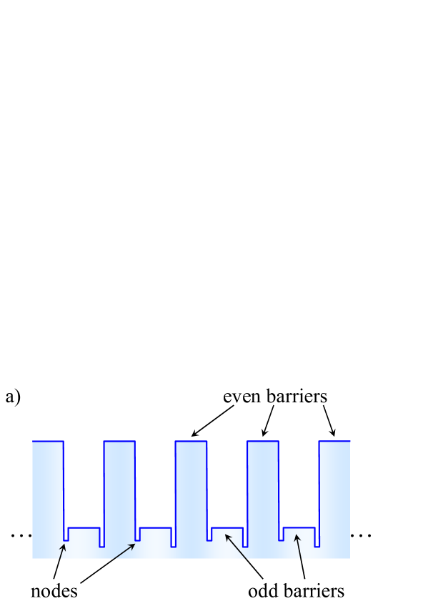
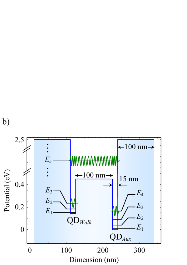
Figure 1: a) An array of quantum dots representing the discrete nodes for a quantum walk on a line. b) The electronic structure of a pair of quantum dots $\text{QD}_{Walk}$ and $\text{QD}_{Aux}$. For the first few energy eigenstates, the overlap between the electron wavefunction inside the dots is negligible.

To implement the quantum walk we use an array of quantum dots, depicted in Fig. 1a, where all the odd barriers have been significantly lowered creating pairs of coupled dots. Figure 1b illustrates a more detailed structure of the pair, labeled as the walk quantum dot $\text{QD}_{Walk}$ and the auxiliary quantum dot $\text{QD}_{Aux}$. The essential feature of this design is that for low energies, the energy eigenstates of $\text{QD}_{Walk}$ and $\text{QD}_{Aux}$ are, to a very good approximation, spatially separable and the electron wavefunction is localized within the dot. For energies above their joint potential barrier however the two dots share common electronic states.

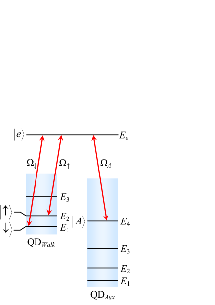
Figure 2: Labeling of the energy levels as coin states $|\downarrow\rangle$ and $|\uparrow\rangle$, excited state $|e\rangle$ and auxiliary state $|A\rangle$. STIRAP operations between states $|\downarrow\rangle\longleftrightarrow|A\rangle$ and $|\uparrow\rangle\longleftrightarrow|A\rangle$ are facilitates via the intermediary state $|e\rangle$, using laser pulses with angular frequencies $\Omega_{\downarrow}$, $\Omega_{\uparrow}$ and $\Omega_{A}$.

The nodes of the quantum walk are mapped to the successive $\text{QD}_{Walk}$ along the array of quantum dots. As depicted in Fig. 2, the first two energy levels of $\text{QD}_{Walk}$ encode the coin states $|\downarrow\rangle$ and $|\uparrow\rangle$ of the walk, the fourth energy level of $\text{QD}_{Aux}$ represents an auxiliary state $|A\rangle$, $E_{e}$ represents an excited state $|e\rangle$ well above the joint barrier between the two dots, and other states remain unoccupied throughout the walk. The quantum walk itself is represented by the propagation of a single electron wavefunction through the array of dots using a series of specially optimized 2- and 3-photon $\Lambda$ STIRAP operations.

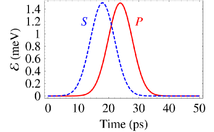
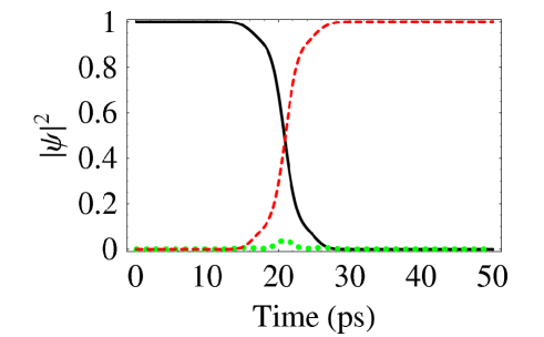
Figure 5: (upper panel) The two laser pulses involved in a 2-photon STIRAP process. Both pulses have a Gaussian envelope and are applied in the counter intuitive order, i.e. the Stokes pulse $S$ responsible for the $|e\rangle\longleftrightarrow|A\rangle$ transition is applied before the pump pulse responsible for the $|\uparrow\rangle\longleftrightarrow|e\rangle$ transition. (lower panel) The time evolution of dressed states $|\uparrow\rangle$ (solid), $|e\rangle$ (dotted) and $|A\rangle$ (dashed) due to the application of the 2-photon STIRAP with pulse parameters optimized to perform a swap operation. Initially $\psi_{\uparrow}=1$ and $\psi_{A}=\psi_{e}=0$.

The 2-photon STIRAP is used to perform the translation operation $\hat{T}^{\uparrow}_{+1}$. Here two laser pulses, pump $P$ and Stoke $S$, with angular frequencies $\Omega_{\uparrow}$ and $\Omega_{A}$ respectively, couple the dressed states $|\uparrow\rangle$ and $|A\rangle$ via the intermediate state $|e\rangle$. By tuning the laser parameters and applying the two pulses in the counter intuitive sequence, one can achieve coherent population transfer between states $|\uparrow\rangle$ and $|A\rangle$ with almost perfect fidelity and without leaving any appreciable papulation residual in state $|e\rangle$ (See Fig. 5).

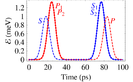
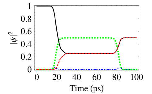
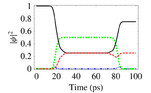
Figure 6: (upper panel) The six laser pulses involved in a 3-photon STIRAP process. All pulses have a Gaussian envelope and are applied in the counter intuitive order. (lower panels) The time evolution of dressed states $|\uparrow\rangle$ (solid), $|\downarrow\rangle$ (dashed), $|e\rangle$ (dot-dashed) and $|A\rangle$ (dotted) with pulse parameters optimized to implement the coin operators $\hat{C}(\nicefrac{{\pi}}{{4}},\nicefrac{{\pi}}{{2}},\nicefrac{{\pi}}{{2}})$ and $\hat{C}(\pi/6,\nicefrac{{\pi}}{{2}},\nicefrac{{\pi}}{{2}})$ respectively. Initially $\psi_{\uparrow}=1$ and $\psi_{\downarrow}=\psi_{A}=\psi_{e}=0$.

Likewise a pair of 3-photon STIRAP is used to perform the coin operation $\hat{C}$. First three laser pulses, $P1$ and $P2$ and $S$, with angular frequencies $\Omega_{\downarrow}$, $\Omega_{\uparrow}$ and $\Omega_{A}$ respectively, couple the dressed states $|\downarrow\rangle$, $|\uparrow\rangle$ and $|A\rangle$ via the intermediate state $|e\rangle$. A second 3-photon STIRAP is then applied in the reverse order. This procedure is shown to be capable of performing arbitrary rotations on the superposition state $\alpha|\uparrow\rangle+\beta|\downarrow\rangle$, independently of the initial amplitudes $\alpha$ and $\beta$ Kis and Renzon (2002) (See Fig. 6). Therefore with careful optimization of laser parameters we can engineer a variety of coin operators $\hat{C}$.

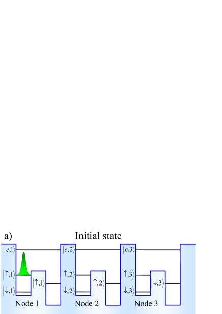
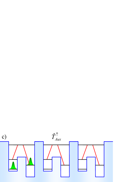
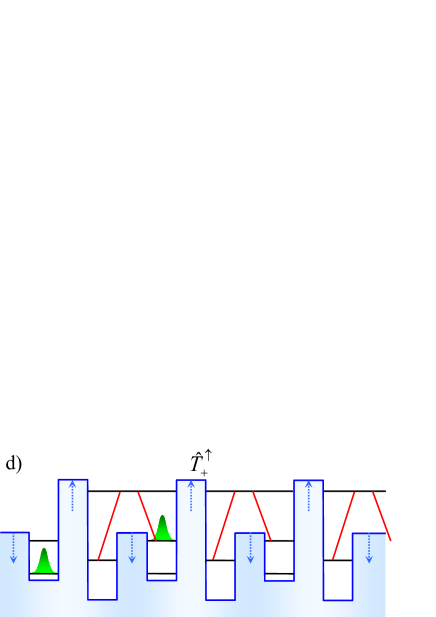
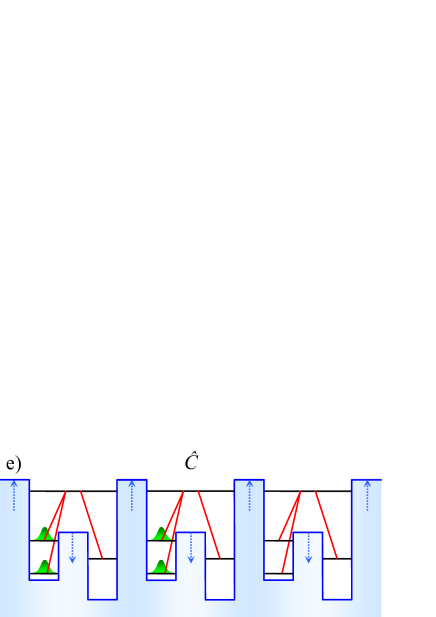
Figure 4: The sequence of 2-photon and 3-photon STIRAP to implement a single step of the quantum walk. a) The initial state of the walk with the electron confined to state $|\uparrow,1\rangle$; b) A 3-photon STIRAP implements the coin rotation $\hat{C}$, mixing the states $|\uparrow,i\rangle$ and $|\downarrow,i\rangle$; c) A 2-photon STIRAP transfers the population from state $|\uparrow,i\rangle$ to state $|A,i\rangle$; d) Even barriers are lowered and odd barriers are raised in order to regroup the quantum dots. It is now possible for another 2-photon STIRAP to transfers the population from state $|A,i\rangle$ to state $|\uparrow,i+1\rangle$, completing the translation operation $\hat{T}^{\uparrow}_{+1}$; e) Potential barriers are returned to their initial setting and the above process repeated.

Figure 4 illustrates how the quantum walk can be performed. First a pair of 3-photon STIRAP operations perform a coin rotation $\hat{C}$ simultaneously on all coin states. A 2-photon STIRAP will then transfer all the $|\uparrow,i\rangle$ states to their corresponding $|A,i\rangle$ state. We then adiabatically raise all the odd barriers and lower the even barriers, virtually reversing the paring of the quantum dots. In this new arrangement every $\text{QD}_{Aux}$ previously associated with the $i$th node is now paired up with $(i+1)$th $\text{QD}_{Walk}$. Using a second 2-photon STIRAP we can now transfer $|A,i\rangle$ to $|\uparrow,i+1\rangle$ which completes the implementation of $\hat{T}^{\uparrow}_{+1}$ operator. The barriers are then returned to their original setting and the process repeated for additional steps. The final quantum walk distribution corresponds to the probability distribution for detecting the electron inside each $\text{QD}_{Walk}$ in the array of dots.

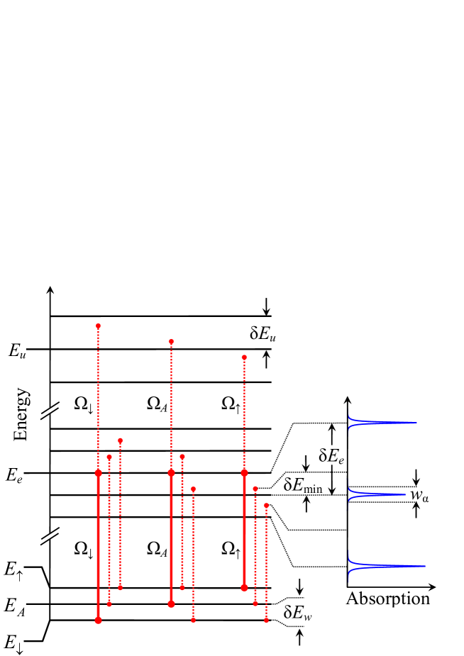
Figure 3: Energy level diagram for a single node corresponding to the quantum dot dimensions presented in Fig. 1: $E_{A}\approx 173$ meV, $E_{e}\approx 1045$ meV and $E_{u}\approx 1912$ meV. Energy levels $E_{\uparrow}$ and $E_{\downarrow}$ are nearly equidistant from $E_{A}$ with an energy gap $\delta E_{w}\approx 15$ meV. Similarly, the immediate levels above and below $E_{e}$ and $E_{u}$ are separated by $\delta E_{e}\approx 20$ meV and $\delta E_{e}\approx 30$ meV respectively. The absorption spectrum is assumed to have a line width $w_{\alpha}\lesssim 1$ meV. Solid lines represent the coupling between the desired energy levels via $\Omega_{\downarrow}$, $\Omega_{\uparrow}$ and $\Omega_{A}$ pulses. Dotted lines demonstrate that these frequencies are prevented by the energy structure from activating any spurious coupling between other any levels.

An important consideration in the design of the quantum dots is the ability to perform selective addressing of states which are being coupled via STIRAP and to avoid all unwanted secondary excitations. Taking, for example, the $\Omega_{\uparrow}$ pulse which is intended to couple the energy levels $E_{\uparrow}$ and $E_{e}$, the quantum dot energy structure should disallow a secondary excited state, say $E_{e^{\prime}}=E_{\downarrow}+\Omega_{\uparrow}\hbar$ to exist, as it would lead to the unwanted excitation of the $E_{\downarrow}$ level. Similarly, to avoid leaking the electron out of the dot via ladder excitations, the energy structure should prevent the coupling of $E_{e}$ to an upper energy level $E_{e}+\Omega_{\uparrow}\hbar$. What is attractive about our proposal is that experimentally this can be achieved without resorting to complex profiles for the quantum dot potential. In fact using simple square wells with dimensions given in Fig. 1b we were able to produce the necessary energy structure depicted in Fig. 3. Assuming absorption line widths $\alpha\lesssim 1$ meV, all superfluous excitations will be far off resonance and will not have any appreciable magnitude.

IV Results

In order to simulate the evolution of the quantum walk in the array of dots, we first tuned our laser parameters to correctly perform the desired $\hat{C}$ rotation and $\hat{T}^{\uparrow}_{+1}$ translation operations. For our 2-photon STIRAP operations we employ pump and Stokes pulses with Gaussian envelopes $\mathcal{E}_{s}(t)$ and $\mathcal{E}_{p}(t)$ and parameterize them using their peak interaction energies $\mathcal{\overline{E}}_{p}$ and $\mathcal{\overline{E}}_{s}$, standard deviations $\sigma_{p}$ and $\sigma_{s}$, phase angles $\alpha_{p}$ and $\alpha_{s}$, and the time interval $\Delta\mathcal{T}$ between the peak interaction energies. The STIRAP process can now be modeled by the time-dependant hamiltonian

$$\hat{H}(t)=\left(\begin{array}[]{ccc}0&\mathcal{E}_{s}(t)e^{i\alpha_{s}}&0\\ \mathcal{E}_{s}(t)e^{-i\alpha_{s}}&0&\mathcal{E}_{p}(t)e^{i\alpha_{p}}\\ 0&\mathcal{E}_{p}(t)e^{-i\alpha_{p}}&0\end{array}\right),$$ (5)

constructed using the Rotating Wave Approximation Shore (1990) in the Raman resonance limit. The pulse parameters need to be tuned such that the resulting 2-photon STIRAP operation coherently transfers an entire population from state $|\uparrow,i\rangle$ to state $|A,i\rangle$ via state $|e,i\rangle$. We achieve this by optimizing $\mathcal{\overline{E}}_{p}$ and $\Delta\mathcal{T}$, using a technique detailed in the appendix, while other parameters are fixed to any desired values. Figure 5 shows the time evolution of the dressed states $|\uparrow,i\rangle$ and $|A,i\rangle$ and $|e,i\rangle$ under the application of the optimized 2-photon STIRAP, where we have set $\mathcal{\overline{E}}_{s}=1.5$ meV, $\sigma_{p}=\sigma_{s}=4.0$ ps and $\alpha_{p}=\alpha_{s}=0$, and the optimum $\mathcal{\overline{E}}_{p}=1.50$ meV and $\Delta\mathcal{T}=5.87$ ps. In order to achieve the second transition from $|A,i\rangle$ to $|\uparrow,i+1\rangle$ (after raising and lowing the alternate potential barriers) we simply reverse the order in which the pump and Stoke pulses are applied.

In the double 3-photon STIRAP process depicted in Fig. 6, the pulse parameters need to be tuned to perform a unitary operation $\hat{C}$ on the coin states. As before we achieve this by optimizing $\mathcal{\overline{E}}_{b}$ and $\Delta\mathcal{T}$ after fixing the other parameters to any desired values. Setting $\mathcal{\overline{E}}_{a}=1.0$ meV, $\sigma=4.0$ ps, $\alpha_{s}=\alpha_{p1}=\beta_{p}=0$, $\alpha_{p2}=\beta_{s1}=\beta_{s2}=\pi$, $\alpha_{p1}=\beta_{s1}=\pi$, $\alpha_{p2}=\beta_{s2}=0$ and $\alpha_{s}=0$, with optimum parameters $\mathcal{\overline{E}}_{b}=1.34$ meV and $\Delta\mathcal{T}=6.12$ ps, we obtain symmetric coins by simply varying $\beta_{p}$. Figure 6 depict the time evolution of the dressed states $|\downarrow\rangle$, $|\uparrow\rangle$, $|A\rangle$ and $|e\rangle$ under the action of the coin operators $\hat{C}(\nicefrac{{\pi}}{{4}},\nicefrac{{\pi}}{{2}},\nicefrac{{\pi}}{{2}})$ and $\hat{C}(\pi/6,\nicefrac{{\pi}}{{2}},\nicefrac{{\pi}}{{2}})$ for $\beta_{p}=\nicefrac{{\pi}}{{2}}$ and $\beta_{p}=\nicefrac{{\pi}}{{3}}$ respectively. We also obtain asymmetric coins like $\hat{C}(\nicefrac{{\pi}}{{4}},\nicefrac{{\pi}}{{2}},-\nicefrac{{\pi}}{{2}})$ by setting $\alpha_{p1}=\beta_{s1}=\pi$, $\alpha_{p2}=\beta_{s2}=\nicefrac{{\pi}}{{2}}$, $\alpha_{s}=0$ and $\beta_{p}=\nicefrac{{\pi}}{{2}}$.

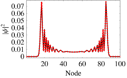
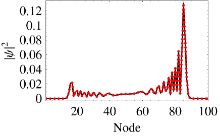
Figure 7: The electron probability distribution after 100 applications of the pulse sequence (solid) vs. the corresponding discrete-time quantum random walk distribution after 100 steps (dotted). The pulse 3-photon pulse parameters were optimized to perform $\hat{C}(\pi/4,\nicefrac{{\pi}}{{2}},\nicefrac{{\pi}}{{2}})$ and the electron was initially confined to node 1 with probability distribution: $\psi_{\uparrow}=\psi_{\downarrow}=\nicefrac{{1}}{{\sqrt{2}}}$ (upper panel) and $\psi_{\uparrow}=1$ and $\psi_{\downarrow}=0$ (lower panel).

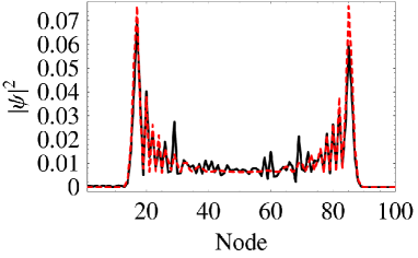
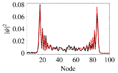
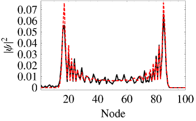
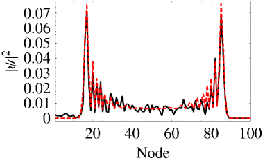
Figure 8: The impact of introducing some noise in the applied pulse parameters. a) Deviation from the exact quantum random walk distribution (dashed) due to an induced 2% uncertainty in the laser pulse peak energies (solid). b) Deviation from the exact quantum random walk distribution (dashed) due to an induced 5% uncertainty in the laser pulse phases (solid). c) Deviation from the exact quantum random walk distribution (dashed) due to an induced 2% uncertainty in the laser pulse standard deviations (solid). d) Deviation from the exact quantum random walk distribution (dashed) due to an induced 0.3% uncertainty in the laser pulse timing (solid).

Following the control pulse optimization, we obtain the full $3\times 3$ and $4\times 4$ evolution matrices corresponding to the 2- and 3-photon STIRAP operations respectively. We then use these to simulate the evolution of a single electron under the repeated applications of the pulse sequence outlined in Fig. 4. In Fig. 7 we have plotted the electron wavefunction after 100 steps, using optimized pulses corresponding to the translation operator $\hat{T}^{\uparrow}_{+1}$ as well as two different coin operators $\hat{C}(\nicefrac{{\pi}}{{4}},\nicefrac{{\pi}}{{2}},\nicefrac{{\pi}}{{2}})$, and $\hat{C}(\nicefrac{{\pi}}{{6}},\nicefrac{{\pi}}{{2}},\nicefrac{{\pi}}{{2}})$. The results are in excellent agreement with their respective ideal theoretical distributions. We also investigated the effect of noise disturbance and experimental uncertainty on the resulting distribution and demonstrated a relatively robust response against imperfect pulse parameters. Figure 8 shows a reasonable degree of fidelity after the introduction of white noise in the energy peak, phase, timing and the standard deviation of the laser pulses.

V Conclusion

We have proposed a physical implementation of a discrete-time quantum random walk using the action of 2- and 3-photon STIRAP operations on an array of quantum dots. We demonstrated that our scheme reproduces the characteristic quantum walk probability distribution which remains observable after the introduction of modest experimental uncertainty in the laser excitations.

Like many other proposed schemes however, our implementation of the quantum walk is essentially a wave interference experiment and does not involve any quantum entanglements. Such implementations come with a cost as the number of resources grows, at best linearly with the number of nodes required for the walk. Furthermore it is generally expected that almost all potentially useful applications of quantum walks such as search algorithms Shenvi et al. (2003) or element distinctness Ambainis (2003), stem from higher dimensional walks on general graphs. Nevertheless implementing one dimensional quantum walks is significant for carrying out feasibility studies of assembling such physical systems.

APPENDIX: Control Pulse Optimization

Considering a time-dependant hamiltonian $\hat{H}(t)$ for the 2-photon STIRAP, its action on a three-level system can be determined by solving the Schrödinger equation

$$\hat{H}\left(\begin{array}[]{c}\psi_{1}(t)\\ \psi_{2}(t)\\ \psi_{3}(t)\end{array}\right)=i\hbar\frac{\partial}{\partial t}\left(\begin{array}[]{c}\psi_{1}(0)\\ \psi_{2}(0)\\ \psi_{3}(0)\end{array}\right).$$ (A-1)

We do this by approximating $\hat{H}(t)$ using a series of time independent $\hat{H}_{i}$ over suitably short time steps $\delta t$, which allows us to write the solution as

$$\left(\begin{array}[]{c}\psi_{1}(t)\\ \psi_{2}(t)\\ \psi_{3}(t)\end{array}\right)=\hat{U}_{T}(t)\left(\begin{array}[]{c}\psi_{1}(0)\\ \psi_{2}(0)\\ \psi_{3}(0)\end{array}\right),$$ (A-2)

where the evolution operator

$$\hat{U}_{T}(t) = e^{-i\hat{H}_{t}\delta t/\hbar}e^{-i\hat{H}_{t-1}\delta t/\hbar}\cdots e^{-i\hat{H}_{2}\delta t/\hbar}e^{-i\hat{H}_{1}\delta t/\hbar}$$ (A-3)

$$= \left(\begin{array}[]{ccc}\hat{u}_{11}&\hat{u}_{12}&\hat{u}_{13}\\ \hat{u}_{21}&\hat{u}_{22}&\hat{u}_{23}\\ \hat{u}_{31}&\hat{u}_{32}&\hat{u}_{33}\end{array}\right).$$ (A-7)

By carefully optimizing the pulse parameters we can achieve

$$\left(\begin{array}[]{cc}\hat{u}_{11}&\hat{u}_{13}\\ \hat{u}_{31}&\hat{u}_{33}\\ \end{array}\right)\simeq\hat{T}=\left(\begin{array}[]{cc}0&1\\ 1&0\\ \end{array}\right),$$ (A-8)

which is the ideal swap operation between states $|1\rangle$ and $|3\rangle$ via the intermediate state $|2\rangle$. When state $|3\rangle$ is initially empty, this amounts to a translation operation which coherently transfers an amplitude from state $|1\rangle$ entirely to the empty state $|3\rangle$ without populating the intermediate state $|2\rangle$.

We achieve the optimization by first fixing $\mathcal{\overline{E}}_{s}$ and phase angles $\sigma_{p}$, $\sigma_{s}$, $\alpha_{p}$ and $\alpha_{s}$, and then varying $\mathcal{\overline{E}}_{p}$ and $\Delta\mathcal{T}$ in order to minimize the cost function

$$\kappa_{T} = \sum\left|\left(\begin{array}[]{cc}\hat{u}_{11}&\hat{u}_{13}\\ \hat{u}_{31}&\hat{u}_{33}\\ \end{array}\right)-\left(\begin{array}[]{cc}0&1\\ 1&0\\ \end{array}\right)\right|$$ (A-13)

$$= \left|\hat{u}_{11}\right|+\left|\hat{u}_{13}-1\right|+\left|\hat{u}_{31}-1\right|+\left|\hat{u}_{33}\right|.$$ (A-14)

The exponentials $e^{-i\hat{H}_{t}\delta t/\hbar}$, which have to be re-evaluated for every parameter variation, are efficiently and accurately computed using a Chebyshev expansion Tal-Ezer and Kosloff (1984); Wang and Midgley (1999)

$$e^{A}=\sum_{n=0}^{\mathcal{N}}a_{n}(\alpha)\phi_{n}(\mathcal{\widetilde{A}}),$$ (A-15)

where $A=-i\hat{H}_{t}\delta t/\hbar$, $a_{n}(\alpha)=2J_{n}(\alpha)$ except for $a_{0}(\alpha)=J_{0}(\alpha)$, $J_{n}(\alpha)$ are the Bessel functions of the first kind, $\phi_{n}$ are the Chebyshev polynomials, and $\mathcal{N}$ is the number of terms in the Chebyshev expansion. To ensure convergence, the exponent $A$ needs to be normalized as

$$\mathcal{\widetilde{A}}=\frac{2A}{\mu_{max}-\mu_{min}},$$ (A-16)

where $\mu_{min}$ and $\mu_{max}$ represent the minimum and maximum eigenvalues of $A$. Chebyshev polynomials $\phi_{n}$ are efficiently evaluated using the recurrence relation

$$\phi_{n}(\mathcal{\widetilde{A}})=2\mathcal{\widetilde{A}}\phi_{n-1}(\mathcal{\widetilde{A}})+\phi_{n-2}(\mathcal{\widetilde{A}}),$$ (A-17)

and

$$\phi_{0}(\mathcal{\widetilde{A}})=1,\text{~{}~{}}\phi_{1}(\mathcal{\widetilde{A}})=\mathcal{\widetilde{A}}.$$ (A-18)

In practice, iterations are continued until the norm of the matrix exponential converges to the required level of accuracy.

The 3-photon STIRAP process is similarly represented by

$$\left(\begin{array}[]{c}\psi_{1}(t)\\ \psi_{2}(t)\\ \psi_{3}(t)\\ \psi_{4}(t)\end{array}\right)=\hat{U}_{C}(t)\left(\begin{array}[]{c}\psi_{1}(0)\\ \psi_{2}(0)\\ \psi_{3}(0)\\ \psi_{4}(0)\end{array}\right),$$ (A-19)

where the evolution operator

$$\hat{U}_{C}(t)=\left(\begin{array}[]{cccc}\hat{u}_{11}&\hat{u}_{12}&\hat{u}_{13}&\hat{u}_{14}\\ \hat{u}_{21}&\hat{u}_{22}&\hat{u}_{23}&\hat{u}_{24}\\ \hat{u}_{31}&\hat{u}_{32}&\hat{u}_{33}&\hat{u}_{34}\\ \hat{u}_{41}&\hat{u}_{42}&\hat{u}_{43}&\hat{u}_{44}\end{array}\right).$$ (A-20)

This time pulse parameters can be optimized in order to to achieve

$$\left(\begin{array}[]{cc}\hat{u}_{11}&\hat{u}_{12}\\ \hat{u}_{21}&\hat{u}_{22}\\ \end{array}\right)\simeq\hat{C},$$ (A-21)

where $\hat{C}$ is a desired unitary coin matrix given by Eq. 1.

As before, this is achieved by fixing all the parameters except for $\mathcal{\overline{E}}_{b}$ and $\Delta\mathcal{T}$ which are varied to minimize the cost function

$$\kappa_{C}=\sum\left|\left(\begin{array}[]{cc}\hat{u}_{11}&\hat{u}_{12}\\ \hat{u}_{21}&\hat{u}_{22}\\ \end{array}\right)\left(\begin{array}[]{cc}\hat{u}_{11}&\hat{u}_{21}\\ \hat{u}_{12}&\hat{u}_{22}\\ \end{array}\right)^{\ast}-\left(\begin{array}[]{cc}0&1\\ 1&0\\ \end{array}\right)\right|.$$ (A-22)

Figure 9 shows the minimization surface profile for the parameters given in Sec. IV. It is important to note that the above cost function leads to a “loose” optimization in the sense that it does not strictly optimize the STIRAP into any specific coin operator. Rather, it only requires that the coin matrix be unitary. It also turns out that the optimum parameters for a unitary $\hat{C}$ are independent of the choice of phase factors $\alpha$ and $\beta$. Instead these phases can be conveniently altered to manipulate the exact form of the operator $\hat{C}$ while maintaining its unitarity.

VI Figures

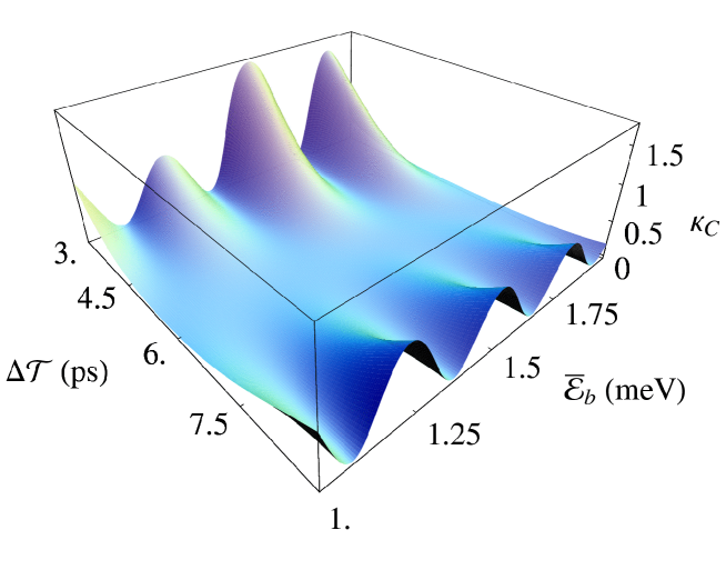
Figure 9: The optimization surface of the $\hat{C}$ operator obtained by minimizing the cost function $\kappa_{C}$ (Eq. A-22). Referring to Fig. 6, $\mathcal{\overline{E}}_{b}$ is the $P1$ pulse energy peak and $\Delta\mathcal{T}$ is the time between the $S$ and $P1$ pulse energy peaks.

References

- Aharonov et al. (1993) Y. Aharonov, L. Davidovich, and N. Zagury, Phys. Rev. A 48, 1687 (1993).
- Farhi and Gutmann (1998) E. Farhi and S. Gutmann, Phys. Rev. A 58, 915 (1998).
- Kempe (2003) J. Kempe, in RANDOM ’03: Proceedings of 7th International Workshop on Randomization and Approximation Techniques in Computer Science (Princeton, NY, USA, 2003), pp. 354–369, eprint arXiv:quant-ph/0205083.
- Childs et al. (2003) A. Childs, R. Cleve, E. Deotto, E. Farhi, S. Gutmann, and D. Spielman, in STOC ’03: Proceedings of the 35th annual ACM Symposium on Theory of Computing (ACM Press, New York, 2003), eprint arXiv:quant-ph/0209131.
- Shenvi et al. (2003) N. Shenvi, J. Kempe, and K. B. Whaley, Phys. Rev. A 67, 052307 (2003).
- Childs and Goldstone (2004) A. Childs and J. Goldstone, Phys. Rev. A 70, 022314 (2004).
- Konno (2005) N. Konno, Phys. Rev. E 72, 26113 (2005).
- Patel et al. (2005) A. Patel, K. S. Raghunathan, and P. Rungta, Phys. Rev. A 71, 32347 (2005).
- Strauch (2006) F. W. Strauch, Phys. Rev. A 74, 030301 (2006).
- Du et al. (2003) J. Du, H. Li, X. Xu, M. Shi, J. Wu, X. Zhou, and R. Han, Phys. Rev. A 67, 042316 (2003).
- Ryan et al. (2004) C. A. Ryan, M. Laforest, J. C. Boileau, and R. Laflamme, Phys. Rev. A 69, 012310 (2004).
- Agarwal and Pathak (2005) G. S. Agarwal and P. K. Pathak, Phys. Rev. A 65, 032310 (2005).
- Sanders and Bartlett (2003) B. C. Sanders and S. D. Bartlett, Phys. Rev. A 67, 042305 (2003).
- Di et al. (2004) T. Di, M. Hillery, and M. S. Zubairy, Phys. Rev. A 70, 032304 (2004).
- Travaglione and Milburn (2002) B. C. Travaglione and G. J. Milburn, Phys. Rev. A 65, 032310 (2002).
- Zhi Zhao and Pan (2002) H. L. T. Y. Z.-B. C. Zhi Zhao, Jiangfeng Du and J.-W. Pan (2002), eprint arXiv:quant-ph/0212149.
- H. Jeong and Kim (2004) M. P. H. Jeong and M. S. Kim, Phys. Rev. A 69, 012310 (2004).
- Do et al. (2005) B. Do, M. L. Stohler, S. Balasubramanian, D. S. Elliott, C. Eash, Ephraim, Fischbach, M. A. Fischbach, A. Mills, and B. Zwickl, Opt. Soc. Am. B 22, 020499 (2005).
- Knight et al. (2003a) P. L. Knight, E. Roldán, and J. E. Sipe, Phys. Rev. A 68, 020301 (2003a).
- Knight et al. (2003b) P. L. Knight, E. Roldán, and J. E. Sipe, Opt. Com. 227, 147 (2003b).
- nuls et al. (2006) M. C. B. nuls, C. Navarrete, A. Pérez, E. Roldán, and J. C. Soriano, Phys. Rev. A 73, 062304 (2006).
- Francisco et al. (2006) D. Francisco, C. Iemmi, J. P. Paz, , and S. Ledesma, Phys. Rev. A 74, 052327 (2006).
- Zou et al. (2006) X. Zou, Y. Dong, and G. Guo, New Jour. Phys. 8, 81 (2006).
- Zhang et al. (2007) P. Zhang, X.-F. Ren, X.-B. Zou, B.-H. Liu, Y.-F. Huang, and G.-C. Guo, Phys. Rev. A 57, 052310 (2007).
- Hillery et al. (2003) M. Hillery, J. Bergou, and E. Feldman, Phys. Rev. A 68, 032314 (2003).
- Feldman and Hillery (2004) E. Feldman and M. Hillery (2004), eprint arXiv:quant-ph/0312062.
- Košík and Bužek (2005) J. Košík and V. Bužek, Phys. Rev. A 71, 012306 (2005).
- Dur et al. (2002) W. Dur, R. Raussendorf, V. M. Kendon, and H. J. Briegel, Phys. Rev. A 66, 052319 (2002).
- Chandrashekar (2006) C. M. Chandrashekar, Phys. Rev. A 74, 032307 (2006).
- Joo et al. (2006) J. Joo, P. L. Knight, and J. K. Pachos (2006), eprint arXiv:quant-ph/0606087 v2.
- Côté et al. (2006) R. Côté, A. Russell, E. E. Eyler, and P. L. Gould, New Jour. Phys. 8, 156 (2006).
- Eckert et al. (2005) K. Eckert, J. Mompart, G. Birkl, and M. Lewenstein, Phys. Rev. A 72, 012327 (2005).
- Solenov and Fedichkin (2006) D. Solenov and L. Fedichkin, Phys. Rev. A 73, 012313 (2006).
- Bergmann et al. (1998) K. Bergmann, H. Theuer, and B. W. Shore, Rev. Mod. Phys. 70, 1003 1025 (1998).
- Král and Shapiro (2001) P. Král and M. Shapiro, Phys. Rev. Lett. 87, 183002 (2001).
- Hohenester et al. (2000) U. Hohenester, F. Troiani, E. Molinari, G. Panzarini, and C. Macchiavello, Appl. Phys. Lett. 77, 1864 (2000).
- Kis and Renzon (2002) Z. Kis and F. Renzon, Phys. Rev. A 65, 032318 (2002).
- Shore (1990) B. W. Shore, The Theory of Coherent Atomic Excitation (Wiley-Interscience, 1990).
- Ambainis (2003) A. Ambainis (2003), eprint arXiv:quant-ph/0311001.
- Tal-Ezer and Kosloff (1984) H. Tal-Ezer and R. Kosloff, J. Chem. Phys. 81, 3967 (1984).
- Wang and Midgley (1999) J. B. Wang and S. Midgley, Phys. Rev. B 60, 13668 (1999).