A random walk approach to quantum algorithms

Abstract

quantum information, quantum computation, quantum algorithms The development of quantum algorithms based on quantum versions of random walks is placed in the context of the emerging field of quantum computing. Constructing a suitable quantum version of a random walk is not trivial: pure quantum dynamics is deterministic, so randomness only enters during the measurement phase, i.e., when converting the quantum information into classical information. The outcome of a quantum random walk is very different from the corresponding classical random walk, due to interference between the different possible paths. The upshot is that quantum walkers find themselves further from their starting point on average than a classical walker, and this forms the basis of a quantum speed up that can be exploited to solve problems faster. Surprisingly, the effect of making the walk slightly less than perfectly quantum can optimize the properties of the quantum walk for algorithmic applications. Looking to the future, with even a small quantum computer available, development of quantum walk algorithms might proceed more rapidly than it has, especially for solving real problems.

1 Introduction

The idea that quantum systems might be able to process information fundamentally more efficiently than our everyday classical computers arose over twenty years ago from visionary scientists such as Feynman (1982) and David Deutsch (1985). They both perceived that a superposition of multiple quantum trajectories looks like a classical parallel computer, which calculates the result of many different input values in the time it takes for one processor to do one input value. Except the quantum system doesn’t need a stack of processors, the parallel processing comes ‘for free’ with quantum dynamics, providing a vast economy of scale over classical computation. For the next ten years this remained a neat idea with no hope of practical application, since the fragile nature of quantum superpositions could not be perfectly controlled to yield a functional quantum computer. Then came two milestone results in quantum computation: error correction (Knill et al. 1996; Aharonov and Ben-Or 1996; Steane 1996) to protect the fragile quantum systems long enough to run a computation, and Shor’s algorithm (Shor 1997) for factoring large numbers, which threatens the security of cryptographic systems. This gave quantum computing both practicality and purpose: the growth in research over the past ten years has been phenomenal on both theoretical and experimental aspects of the challenge to construct a working quantum computer.

A quantum computer requires both hardware and software. Both are proving to be fascinating areas of research, with many beautiful results appearing at each step of the process. In terms of size, the hardware is not very far advanced: we cannot even manipulate as many as ten qubits (quantum bits) long enough to do a simple calculation a child could do in their head. But this belittles the exquisite control over single particles that has been developed in a diverse set of fields from photons to trapped atoms and ions to quantum dots to electrons floating on liquid helium to nuclear spins to SQUIDS (superconducting quantum interference devices), see Spiller et al. (2005) for a recent review. Progress has been steady and impressive: nothing has yet been discovered in all these experiments that says we cannot expand them as far as is necessary to make a useful quantum computer.

The software side is also at a relatively early stage. Shor’s factoring algorithm is the first in a family of quantum algorithms based on Fourier transforms, which exploit the fact that a quantum computer can calculate a Fourier transform efficiently for many different inputs in superposition then extract a common periodicity from the result. In technical terms, the task is to identify a hidden subgroup in the group structure of the problem (Lomont 2004, provides a recent review). This works well for Abelian groups, but extending the method to a non-Abelian groups, where some of the notorious hard problems, such as graph isomorphism, lie, is proving tricky. The parallelism of quantum systems may come ‘for free’, but extracting the answer does not. When a quantum superposition is measured, it only gives out a single randomly selected result from the many it is holding. One therefore has to be very ingenious about how to arrange the superposition prior to the measurement in order to maximize the chance of obtaining the required information.

Clearly we’d like to find many more methods for programming a quantum computer. One obvious place to look is where classical algorithms are having the most success, to see if a quantum version could be even faster. Randomized algorithms are one such arena, they provide the best known methods for approximating the permanent of a matrix (Jerrum et al. 2001), finding satisfying assignments to Boolean expressions ($k$SAT with $k>2$) (Schöning 1999), estimating the volume of a convex body (Dyer et al. 1991), and graph connectivity (Motwani and Raghavan 1995). Classical random walks also underpin many standard methods in computational physics, such as Monte Carlo simulations. There are two approaches to quantum versions of random walks: Farhi and Gutmann (1998) investigated quantum walks using a discrete space (lattice or graph) with a continuous-time quantum dynamics, and Aharanov, D et al. (2001) studied quantum walks with both space and time discretized. Within a few years, the first proper algorithms using quantum walks appeared from Childs et al. (2003) and Shenvi et al. (2003), and more have since followed: for a short survey see Ambainis (2003).

In this paper we will review how the simplest quantum walk behaves in comparison with a classical random walk, then briefly describe the two above-mentioned quantum walk algorithms. We will then turn to more basic questions about how quantum walks work, including the effects of making them slightly imperfect. Finally, we will consider the possible future of quantum walk algorithms in the context of the prospects for practical quantum computing.

2 A simple quantum walk

Lets start with a random walk on a line – a drunkard’s walk – where the choice of whether to step to the right or the left is made randomly by the toss of a coin. A step-by-step set of instructions for a classical random walk is given in table 1 in the left-hand column. As is well known, after taking $t$ random steps, the average distance from the starting point is $\sqrt{t}$ steps.

Table 1: Recipes for a classical random walk (left) and a quantum random walk (right) on a line. The symbol $|x,c\rangle$ denotes a quantum walker at position $x$ with a coin in state $c$. The quantum operations $\mathbf{H}$ and $\mathbf{S}$ are defined by their effect on $|x,c\rangle$ as given below.

Classical random walk	Quantum walk
1. start at the origin: $x=0$	1. start at the origin: $x=0$
2. toss a coin	2. toss a qubit (quantum coin)
result is head or tail	$\mathbf{H}|x,0\rangle\longrightarrow(|x,0\rangle+|x,1\rangle)/\sqrt{2}$
	$\mathbf{H}|x,1\rangle\longrightarrow(|x,0\rangle-|x,1\rangle)/\sqrt{2}$
3. move one unit left or right	3. move one unit left and right
according to coin state:	according to qubit state
tail: $x\longrightarrow x-1$	$\mathbf{S}|x,0\rangle\longrightarrow|x-1,0\rangle$
head : $x\longrightarrow x+1$	$\mathbf{S}|x,1\rangle\longrightarrow|x+1,1\rangle$
4. repeat steps 2. and 3. $t$ times	4. repeat steps 2. and 3. $t$ times
5. measure position $-t\leq x\leq t$	5. measure position $-t\leq x\leq t$
6. repeat steps 1. to 5. many times	6. repeat steps 1. to 5. many times
$\longrightarrow$ prob. dist. $P(x,t)$, binomial	$\longrightarrow$ prob. dist. $P(x,t)$ has
standard deviation $\langle x^{2}\rangle^{1/2}=\sqrt{t}$	standard deviation $\langle x^{2}\rangle^{1/2}\propto t$

Naïvely, for a quantum version of this based on the Feynman/Deutsch view of quantum computation as parallel processing, one would expect to follow all the possible random walks in superposition, instead of just one particular sequence of steps. At each step, then, move left and right in equal amounts, repeating this until the quantum walker is smeared out along the line in the same distribution as one finds after many trials with a classical random walk.

However, this isn’t possible within the constraints of quantum dynamics, as shown by Meyer (1996). Pure quantum dynamics must be unitary, which means being completely deterministic and reversible. The naïve superposition of all possible random walks is not reversible, you can’t tell which way you arrived at a particular location, so you don’t know which way to step to go back. The solution is to make the coin quantum too, and give it a unitary twist instead of a random toss. The quantum coin keeps track of which way you arrived at your location, allowing you to retrace your steps. This recipe for a quantum walk was first investigated with algorithmic applications in mind by Aharanov, D et al. (2001) and Ambainis et al. (2001). Table 1 compares the instructions for performing classical and quantum random walks on a line. The shape of the distributions obtained is shown in figure 1.

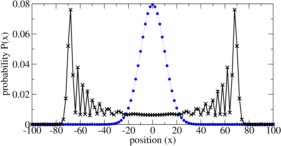
Figure 1: Comparison of quantum (crosses) and classical (circles) walks on a line, after 100 steps. Only even points are shown since odd points are unoccupied at even time steps.

The quantum walk looks nothing like the binomial distribution of the classical random walk. But we have gained something significant: the quantum walk spreads faster, at a rate proportional to the number of steps, instead of the square root of the number of steps as in the classical case, a quadratic speed up.

3 Quantum walk algorithms

Of course, quadratically faster spreading on a line isn’t an algorithm yet, but it is a good start, and soon Shenvi et al. (2003) showed that a quantum walk could search an unsorted database with a quadratic speed up. The first quantum algorithm for this problem is due to Grover (1996), using a different method to obtain the same quadratic speed up. A classical search of an unsorted database (e.g., starting with a phone number and searching a telephone directory to find the corresponding name), potentially has to check all $N$ entries in the database, and on average has to check at least half. A quantum search only needs to make $\sqrt{N}$ queries, though the queries ask for many answers in superposition. The quantum walk search algorithm sort of works backwards, starting in a uniform superposition over the whole database, and converging on the answer as the quantum walk proceeds. As already noted, quantum walks are reversible: a quantum walk running backwards is also a quantum walk.

Childs et al. (2003) proved that a quantum walk could perform exponentially faster than any classical algorithm when finding a route across a particular sort of network, see figure 2. This is a rather artificial problem, but proves in principle that quantum walks are a powerful tool.

Figure 2: (Small) example of the network in Childs et al. (2003). The gap between columns 4 and 5 is for clarity only, the length of the paths is the same between all nodes.

The task is to find your way from the entrance node to the exit node, treating the rest of the network like a maze where you cannot see the other nodes from where you stand, only the choice of paths. It is easy to tell which way is forward until you reach the random joins in the centre. After this, any classical attempt to pick out the correct path to the exit get lost in the central region and takes exponentially long, on average, to find the way out. A quantum walk, on the other hand, travels through all the paths in superposition, and the quantum interference between different paths allows the quantum walker to figure out which way is forward right up to the exit, which it finds in time proportional to the width of the network. Childs et al. (2003) use a continuous time quantum walk for this algorithm. The recipes for continuous time walks are similar to the discrete time walks in table 1. Continuous time walks do not use a coin: the coin toss and conditional shift (steps 2. and 3.) are replaced by a hopping rate $\gamma$ per unit time for the probability of moving to a neighbouring location, and step 4. by continuous evolution for a time $t$, see Farhi and Gutmann (1998).

4 Decoherence in quantum walks

Our quantum walks do not involve any random choices, and they have very different outcomes to classical random walks, so why are they a good quantum analogue of a classical random walk? The similarity of the recipes in table 1 should convince you that the choice is at least a plausible one. One might also reasonably require that the quantum walk reduces to the classical walk ‘in the classical limit’. By this we usually mean the limit obtained by making the system bigger and bigger, until Planck’s constant $h=6.6\times 10^{-34}$Js is very small compared to the energy and time scales in the system. We can’t apply this directly to our quantum walks, but another way to transform to a classical dynamics is by applying decoherence to destroy the quantum correlations that allow the quantum superpositions to exist.

Decoherence is essentially an interaction with the environment, in which the correlations within the system are transformed into correlations with the environment that we can no longer access or control. We can mimic this by measuring our quantum system: this correlates it with our measuring apparatus, but since the measuring apparatus is big enough to be classical in the sense of $h\rightarrow 0$, it forces our quantum walker to a classical state too, removing any quantum superpositions. If we measure the walker after each step, we will find it in just one location on the line, and because the quantum coin toss gives equal probability of moving left and right, we will find the walker one step to the left or right of where it was when we measured the previous step, with equal probability. This is exactly the recipe for a classical random walk, so our quantum walk recipe passes the test. In fact, this is the best definition we have of a quantum walk: a quantum dynamics that reduces to a classical random walk when completely decohered. There are many different examples of classical random walks, and no convenient quantum definition is known that covers everything that reduces to them. One may even start from classical random walks and quantize them (see, for example, Szegedy 2004).

In this sense, then, decoherence is absolutely basic to the definition of a quantum walk. But in a practical sense, decoherence is irrelevant for quantum walk algorithms. When constructing a physical quantum computer, we have to worry a great deal about decoherence, and build in enough error correction to allow the quantum computation to proceed without any errors. If we run our quantum walk algorithm on a quantum computer, just as with our classical computers, we should expect a properly functioning quantum computer to carry out the algorithm without any mistakes due to the action of the environment on the physical computer.

This is not the end of the story on decoherence in quantum walks. When asked whether decoherence would spoil a quantum walk, I thought: silly question, but, somehow that spiky quantum distribution has to turn into the smooth classical one: I wonder how it does it? The answer is in figure 3:

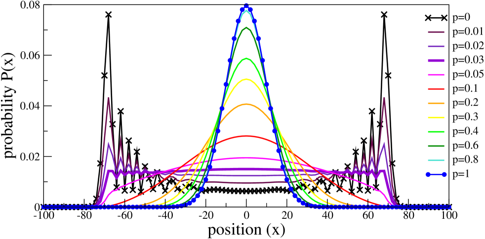
Figure 3: A quantum walk on a line of 100 steps is progressively decohered by random measurements with probability $p$ per time step as given in the key. for $p=0.03$, an approximately ‘top hat’ distribution is obtained (from Kendon and Tregenna 2003).

down come the spikes and up goes the central peak as the decoherence rate is turned up. And in between it passes through a good approximation of a ‘top hat’ distribution, which, for computational physicists who use random walks to sample distributions, is a very desirable feature, since it provides uniform sampling over a specific range.

Inspired by this result, Kendon and Tregenna (2003) also checked what happens to quantum walks on cycles. These are what you get if you take a line segment of length $N$ and join the ends to make a loop. The quantum walk goes round and round in both directions and, unlike a classical random walk, which settles down to within epsilon of a uniform distribution after a certain length of time – the mixing time – a quantum walk continues to oscillate indefinitely. Mixing is needed for uniform random sampling. The shorter the mixing time the more frequently you can sample, and the quicker you obtain a good estimate of the answer to your problem. If quantum walks don’t mix at all, this seems to be useless for algorithms. Fortunately, there is a simple remedy: we define an average distribution

$$\overline{P(x,T)}=\frac{1}{T}\sum_{t=1}^{T}P(x,t).$$ (1)

Operationally, this just means randomly choosing a value of $t$ between $1$ and $T$, then measuring the position of the quantum walker after $t$ steps instead of after $T$ steps. This time-averaged distribution does settle down after an initial mixing time. It does not necessarily settle to the uniform distribution, though (Aharanov, D et al. 2001), unlike the classical random walk which always mixes to a uniform distribution. This is thus another striking difference between quantum and classical random walks. However, if one uses odd-sized cycles, then the quantum walk does mix to uniform, and Aharanov, D et al. (2001) proved that they mix almost quadratically faster than classical random walks (in time proportional to $N\log N$ steps or better, compared to $N^{2}$ steps). Applying decoherence to a quantum walk on a cycle causes it to mix even faster than a pure quantum walk, and to always mix to a uniform distribution (Kendon and Tregenna 2003). So again, like the top hat distribution, decoherence seems to enhance the useful quantum features. Recent work by Richter (2006) suggests that the enhancement is linked to an amplification technique first applied to quantum walks by Aharanov, D et al. (2001).

However, quantum walks on other structures, such as the hypercube, do not necessarily mix faster than classical random walks, (Moore and Russell 2002). Such effects may be dependent on the structure having a favourable symmetry Krovi and Brun (2006); Keating et al. (2006). The real lesson to take from this is that we do not have to be restricted to pure quantum dynamics when designing algorithms, we have far more tools at our disposal to tune and optimize our quantum walk to suit the problem at hand. Indeed, the idea that measurements form an integral part of the quantum computational process has been suggested in several contexts (for an overview see Jozsa 2005b), in particular the cluster state model by Raussendorf and Briegel (2001), And in practical situations, a constant factor of (say) 100 makes a big difference to what can be achieved with a computer of fixed size, so algorithmically insignificant effects may still be valuable once usable quantum computers are available.

5 What makes a quantum walk ‘quantum’?

How does the quantum walk ‘go faster’ than a classical random walk? Those readers familiar with wave dynamics (in whatever context) will have recognized the interference that is occurring between different paths taken by the quantum walker. Here it is in three steps of the quantum walk on a line. Our notation is the same as in table 1, with $|x,c\rangle$ denoting a quantum walker at location $x$ with a quantum coin in state $c$. As defined in table 1, $\mathbf{H}$ is the quantum coin toss operator, and $\mathbf{S}$ is the quantum step operator:

t=0        $$|0,0\rangle$$

t=1 apply $$\mathbf{H} \longrightarrow(\mbox{$|0,0\rangle$}+\mbox{$|0,1\rangle$})/\sqrt{2}$$

apply $$\mathbf{S} \longrightarrow(\mbox{$|{-1},0\rangle$}+\mbox{$|1,1\rangle$})/\sqrt{2}$$

t=2 apply $$\mathbf{H} \longrightarrow(\mbox{$|{-1},0\rangle$}+\mbox{$|{-1},1\rangle$}+\mbox{$|1,0\rangle$}-\mbox{$|1,1\rangle$})/2$$

apply $$\mathbf{S} \longrightarrow(\mbox{$|{-2},0\rangle$}+\mbox{$|0,1\rangle$}+\mbox{$|0,0\rangle$}-\mbox{$|2,1\rangle$})/2$$

t=3 apply $$\mathbf{H} \longrightarrow(\mbox{$|{-2},0\rangle$}+\mbox{$|{-2},1\rangle$}+\mbox{$|0,0\rangle$}-\mbox{$|0,1\rangle$}$$ (2)

$$\hbox{}\hskip 93.00017pt+\mbox{$|0,0\rangle$}+\mbox{$|0,1\rangle$}+\mbox{$|2,0\rangle$}-\mbox{$|2,1\rangle$})/\sqrt{8}$$

$$\mbox{\hbox{}\hskip 6.99997pt}=(\mbox{$|{-2},0\rangle$}+\mbox{$|{-2},1\rangle$}+2\mbox{$|0,0\rangle$}+\mbox{$|2,0\rangle$}-\mbox{$|2,1\rangle$})/\sqrt{8}$$

apply $$\mathbf{S} \longrightarrow(\mbox{$|{-3},0\rangle$}+\mbox{$|{-1},1\rangle$}+2\mbox{$|{-1},0\rangle$}+\mbox{$|1,0\rangle$}-\mbox{$|3,1\rangle$})/\sqrt{8}$$

In step 3, the component with the coin in state $|1\rangle$ at the origin is eliminated while the component with coin state $|0\rangle$ is enhanced. This is such a simple effect, entirely due to the wave nature of quantum mechanics, that the need for a quantum system to gain the speed up, rather than a wave system such as classical light, has been questioned by Knight et al. (2003). Indeed, the experiment with classical light has already been done by Bouwmeester et al. (1999).

To properly address this question, we need to distinguish two different contexts: physical systems, and algorithms. Table 2 shows examples of random walks in various settings.

Table 2: Examples of random walks.

	quantum	classical
physical	atom in optical lattice	snakes and ladders (board game)
computer	glued trees algorithm	lattice QCD calculation

Lined up side by side like this, the distinctions between them should be obvious, but notice that classical computer simulations of all four examples have also been done. Dür et al. (2002) used simulation to assess the effects of errors when making an atom in an optical lattice perform a quantum walk. A quick search on the Internet finds a number of online snakes and ladders games you can play (e.g., http://www.bonus.com/bonus/card/SnakesandLadders.html). Simulations of quantum walk algorithms are described in Tregenna et al. (2003), and the one that seems silliest – classical simulation of a classical computer algorithm – is actually the most useful, for development of software to run on new parallel computers for lattice QCD calculations, Boyle et al. (2003).

For physical systems we can give a straightforward answer to the question of what makes a quantum walk ‘quantum’: like all quantum systems they should exhibit complementarity (Bohr 1928, 1950). The text-book complementarity experiment is Young’s double-slits, in which quantum particles (such as photons or electrons) are thrown through a pair of closely spaced slits, with a device that can detect which slit they pass through. If the particles pass through the slits unobserved, an interference pattern builds up from many particles arriving sequentially, conversely, if we observe which slit they pass through, the interference pattern disappears, corresponding to the wave and particle natures of quantum particles respectively. Although early descriptions of complementarity concern mutually incompatible measurements, Wootters and Zurek (1979) presented a description in which complementarity can be quantified as a trade-off between knowledge about which way each particle goes vs the sharpness of the interference pattern.

Quantum walks can be viewed as just a more complicated set of paths than a double-slit, so, to demonstrate complementarity in a quantum walk, we need to show the trade-off between quantum interference and knowledge of the path taken by the walker. This is just an extension of what was used in section 4 to show a quantum walk reduces to a classical random walk when decohered. We modeled decoherence by applying measurements of the path with probability $p$. If we now view $p$ as a coupling strength between our measuring device and the walker, we are doing a weak, or partial, measurement through which we learn only partial information about the path of the walker. Kendon and Sanders (2004) discuss in detail how to do this, using ancillae to couple the measuring device to the walker, as shown in figure 4.

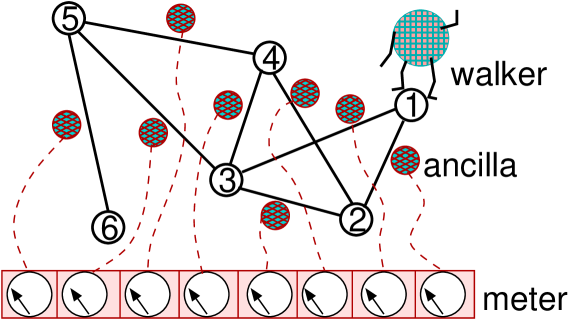
Figure 4: Quantum walker on a general graph with ancillae to measure the path.

An optical system can also exhibit complementarity, since light is not classical, it is made up of many photons. Photons do not interact with each other, so we can consider each photon in a ‘classical’ light beam as doing an independent quantum walk. The optical quincunx experiment (Bouwmeester et al. 1999) is thus a quantum walk experiment in which only the wave nature of light is demonstrated. To also demonstrate the particle nature of light would not be easy, but a possible approach using very low light levels (essentially one photon at a time) is discussed in Kendon and Sanders (2004). On the other hand, water waves could only reproduce the wave nature of a quantum walk, since the underlying particles are not behaving independently, and the wave nature of water arises out of their collective behaviour.

6 Algorithmic efficiency

We will now consider the question of what makes a quantum walk algorithm more efficient than a classical algorithm. A detailed answer is beyond the scope of this paper, being the substance of a major branch of computer science, but we can give a flavour of what is involved. An algorithm is an abstract mathematical concept, whereas we want to consider how efficiently we can run an algorithm on a computer of some sort. Computer scientists do this by associating a cost with each step of the algorithm and with the amount of memory required, embodying the idea that physical computers have a finite size (memory) and work at a finite rate of elementary calculation steps per unit time. This gives us a way to determine if one algorithm is intrinsically faster than another. However, if we want to compare algorithms run on quantum or classical computers, we also need to compare computers: the fundamental way to do this is to ask whether one computer can simulate another with only a constant extra overhead in computation. If so, then they are equivalent for computer science purposes (though not necessarily for practical purposes). In most cases, ‘efficient’ means the algorithms or computers are equivalent to within a factor that scales as a simple polynomial (like $N^{2}$) of the size $N$ of the system, or the number of steps it takes to run the algorithm.

If we could simulate a quantum algorithm efficiently on a classical computer, we would immediately have a classical algorithm that is sufficiently good to render the quantum algorithm superfluous. This is a criterion regularly applied in quantum computing, e.g. the Clifford group of operations can all be efficiently classically simulated, Aaronson and Gottesman (2004), so they are not sufficient to build a quantum computer. Quantum algorithms with no efficient classical simulation may still be equaled or bettered by a classical algorithm using a different method. To prove an algorithmic speed up for a quantum algorithm, we have to prove that no classical algorithm of any type can do as well: such proofs are in general very difficult. Childs et al. (2003) do prove their quantum algorithm is faster than any classical algorithm, but Shor’s algorithm (Shor 1997) is only the ‘best known’ algorithm for factoring, there is no proof something faster can’t be found in future.

6.1 Simulation of classical systems

Broadly speaking, a computer simulation of a physical system is useful if it can be calculated significantly faster and with less resources than just observing the physical system itself. For example, calculating the trajectory of a space probe that takes five years to reach its destination is crucial: we cannot just launch many test probes and see where they end up in order to work out which trajectory we want. Conversely, simulation of fluid flow is not so efficient, and wind tunnel testing is often used for aircraft and turbine design.

One key difference between a classical physical system and a computer simulation of it is that we represent it by binary numbers in a register in the computer. Thus, for our random walks on a line, we need only $\log_{2}N$ bits in our register for each $N$ points on the line. This is an exponential saving in resources. We still need to do $T$ steps of our random walk, so there is no saving in the running time of the program, but we can find out where the walker ended up by making just $log_{2}N$ measurements, each with a binary outcome (zero or one), in contrast to the physical system where we potentially have to examine all of the $N$ positions on the line to discover where the walker ended up. This binary encoding in a computer, compared to unary in a physical system, applies equally to classical and quantum digital computers. In the quantum context it was first remarked on by Jozsa (1998), and Blume-Kohout et al. (2002) presented explicit calculations of the most efficient way to use quantum systems as registers (they don’t need to be binary).

Of course, we don’t get something for nothing: there is a trade off for the exponentially smaller resources of the binary encoding. When we update the state of our random walker, we know that it can only move one step at a time. On the physical line, these steps are to nearest neighbouring points, but in the computer register, going from position ‘7’ to position ‘8’ is $0111\longrightarrow 1000$ in binary, so every one of the bits has to flip, the elementary operations are no longer ‘local’ to a small portion of the space. The price we pay (flipping up to $log_{2}N$ bits compared to a single hop on the line) is still in general a better deal than using exponentially more space to accommodate the whole $N$ points.

6.2 Simulation of quantum systems

The reason why quantum systems are generally hard to simulate with a classical computer is because of the quantum superpositions that all have to be kept track of, the original motivation for quantum computing. The Hilbert space of a quantum system is exponentially bigger than the phase space of a classical system with the same number of degrees of freedom. The numbers get fantastically large. A ten (classical) bit register can be in any one of $2^{10}$ different states. A ten qubit register can be in superposition of all of those $2^{10}$ states at once, with any proportion you like of each state. The quantum computer with a ten qubit register can thus perform up to $2^{10}$ calculations in parallel, each corresponding to a different input state. A hundred qubit computer can do $2^{100}$ calculations at the same time, more than there are particles in the universe (estimated to be around $2^{87}$). Again, of course, there is a trade off for this enormous parallelism. You only get one answer out, not $2^{10}$. A classical computer simulation of a ten qubit quantum computer is easily done with today’s computing power, and it can tell you what the whole superposition is at any stage of the computation, including all $2^{10}$ possible answers, so it is significantly more powerful in terms of the information it makes available.

A quantum simulation of a quantum system can be done efficiently. This is not a trivial statement. It is necessary to show, as Lloyd (1996) did, that if one maps the Hilbert space of the quantum system directly onto the Hilbert space of the quantum register (no binary encoding needed here), then it is possible to simulate the Hamiltonian evolution of the quantum system to sufficient accuracy using a sequence of standard Hamiltonians applied to the quantum register, each for short period of time. Quantum simulation has already been demonstrated (Somaroo et al. 1999), for small systems using NMR quantum computers. However, like classical analogue computing, quantum simulation has a problem with accuracy, which does not scale efficiently with the time needed to run the simulation, Brown et al. (2006).

6.3 Analogue computing

The discussion up until now has implicitly assumed we are discussing digital computers, but this leaves out an important piece of the puzzle. Classical analogue computers go back to Shannon (1941), who showed how they can solve differential equations, given the boundary conditions as inputs. Using a system of non-linear boxes with lots of feedback, they can do this very efficiently; general purpose analogue computers can be constructed with a small number of such boxes that will approximate any differential equation to arbitrary accuracy, Rubel (1981). It is also possible to extend the original concept (e.g., Rubel 1993) to solve a wider class of equations. Analogue computers do not binary encode their data, e.g., the inputs might be directly related to the size of a voltage, and the answer is obtained by measuring the outputs of a suitable subset of the non-linear boxes. The answer is thus as accurate as it is possible to make these measurements, and extra accuracy has an exponential cost compared to digital computing. Rubel (1989) proved that a classical digital computer can simulate an analogue computer, but the reverse question of whether an analogue computer can simulate a digital computer efficiently is open. The utility of analogue computers is in their speed: though they are now rare given the power of today’s digital computers, research continues, and the combination of an analogue ‘chip’ in a digital computer to perform specific real-time operations such as video rendering is one of many possible new applications.

The relevance of analogue computing to quantum computing has not been fully explored, (Jozsa 2005a). Quantum systems accomplish their feats of superposition through an analogue quality: a qubit may be in any superposition of zero and one,

$$\mbox{$|\psi\rangle$}=\alpha\mbox{$|0\rangle$}+\beta e^{i\phi}\mbox{$|1\rangle$},$$ (3)

where $\alpha$ and $\beta$ are real numbers satisfying $\alpha^{2}+\beta^{2}=1$ and $0\leq\phi<2\pi$. The quantum operations we apply to perform a quantum computation alter the values of $\alpha$, $\beta$ and $\phi$, and we can only do this to a finite accuracy. For digital quantum computing, analysis of the effects of limited accuracy in the quantum gates (for example, Nielsen and Chuang 2000, on Shor’s algorithm) suggest it does not affect the computation significantly, but as already mentioned, for quantum simulation the errors scale less favorably (linear in the size of the problem, Brown et al. (2006)).

7 The future of quantum walk algorithms

We do not yet know if we can build a quantum computer large enough to solve problems beyond the reach of the classical computational power available to us, but the rewards for success are so exciting that the challenge is well worth the sustained effort of many years of research by hundreds of talented scientists around the world. And should we find out it is fundamentally impossible to build such a machine, that in itself will tell us crucial facts about the way our universe works.

The first useful application for quantum computers is likely to be simulation of quantum systems. Small quantum simulations have already been demonstrated, and useful quantum simulations – that solve problems inaccessible to classical computation – require less qubits than useful factoring, and may be achievable within five to ten years. A useful digital quantum computer for factoring will need to create and maintain a complex superposition of at least a few thousand qubits. Aaronson (2004) provides a quantitative estimate of what this might mean, against which we can measure experimental achievements. Such a computer is probably ten to twenty years away from realization.

However, quantum walk algorithms may be among the first algorithms to provide useful computation beyond quantum simulation, both because of the wide range of important problems they can be applied to, and their versatility for optimizing their performance. In making this prediction I have a parallel to draw on from classical algorithms, in the development of lattice gas methods for simulating complex fluids. The original idea was first published by Hardy et al. (1973), but had a major shortcoming: on a square or cubic lattice, too many quantities are conserved. The solution (add diagonals to the lattice) came fifteen years later from Frisch et al. (1987), when the development of computers meant that testing and actual use of such methods was within reach. Practical computational methods proceed with a mixture of theory and refinement through testing real instances on real computers. For quantum walks we only have the theory, and simulation on classical computers. This is not enough to fully develop useful applications, and I expect the availability of a working quantum computer to speed up the development of quantum walk algorithms significantly.