Transient localization in the kicked Rydberg atom

Abstract

We investigate the long-time limit of quantum localization of the kicked Rydberg atom. The kicked Rydberg atom is shown to possess in addition to the quantum localization time $\tau_{L}$ a second cross-over time $t_{D}$ where quantum dynamics diverges from classical dynamics towards increased instability. The quantum localization is shown to vanish as either the strength of the kicks at fixed principal quantum number or the quantum number at fixed kick strength increases. The survival probability as a function of frequency in the transient localization regime $\tau_{L}<t<t_{D}$ is characterized by highly irregular, fractal-like fluctuations.

I Introduction

The quantum mechanics of classically chaotic few-degrees of freedom systems has become an intensively studied in the field of “quantum chaos” stock ; cas87 . One key feature is quantum localization, i.e. the localization of the quantum wavefunction while the corresponding classical distribution shows diffusion stock ; cas87 ; berry . In periodically driven systems, this effect has primarily been studied in the kicked rotor, e.g. cas79 ; fish ; adachi ; rotor , and in the Rydberg atom in a sinusoidal electric field, e.g. jensen ; bay ; koch ; buch98 ; buch95 ; leo . For both systems, quantum localization is closely related to Anderson localization in transport in disordered systems cas87 ; buch98 ; fish . One signal of this analogy are strong fluctuations in the quantum system for different observables when varying some external parameter. A third system experimentally and theoretically studied is the periodically kicked Rydberg atom (e.g. jones ; frey ; brom ; burg89 ; hill ; KleSch ; bucks ; noordam ; yo00 ; reinhold04 ), i.e. a hydrogen like atom prepared in a high-lying state and subjected to a sequence of ultra-short impulses. In a recent publication, we showed the existence of quantum localization in the positively kicked Rydberg atom eper03 , i.e. the hydrogenic system with the initial state prepared in a highly elongated quasi-one dimensional state localized on one side of the nucleus and the periodic impulsive momentum transfer $\Delta p>0$ pushing the electron away from the nucleus. The classical phase space of this system is globally chaotic with all tori destroyed for arbitrarily small $\Delta p$, and the classical survival probability decays algebraically, $P_{\rm sur}\propto t^{-\alpha}$, with $\alpha\approx 1.5$ (see Fig. 1 and hill ). In contrast, by following the time-dependent system up to a few thousands of kicks we could show both the quantum suppression of classical ionization and the “freezing out” of the wavefunction, the hallmarks of quantum localization. Several issues remained open, however. They include 1) The origin of a slow, yet noticeable, decay of the localized states, 2) the dynamical role of high harmonics (up to infinity) present in the system, and 3) the properties of strong fluctuations present in the localization regime.

In the following paper we address these issues. We identify two characteristic time-scales (“break times”) in this system. In addition to the localization time $\tau_{l}$, where quantum and classical dynamics begin to differ from each other due to universal destructive interferences, there is a second break time $\tau_{D}$ where localization is broken. Beyond $\tau_{D}$, a second cross-over occurs where the classical dynamics becomes more stable. This second cross-over in the kicked atom is related to the presence of non-classical photoionization.

In the next section, Sect. II, we describe the method used in our studies and in Sect. III we show that quantum localization in the kicked Rydberg atom is transient. Strong fluctuations in the survival probability as a function of frequency for fixed times are studied in Sect. IV and in the last section (Sect. V) a summary is given.

II Method

The Hamiltonian of the one-dimensional kicked Rydberg atom is (in atomic units)

$$H(t)=H_{0}-q\Delta p\sum_{k=1}^{K}\delta(t+T/2-kT)\;,$$ (1)

where $H_{0}=\frac{p^{2}}{2}-\frac{1}{q}$ is the hydrogen Hamiltonian and $q$ the position of the electron. $\Delta p$ and $T$ are the strength and the period of the train of kicks, respectively. We will use the number $K$ of kicks and time $t=K\times T$ interchangeably. The restriction to a 1D model in the present context is necessary since the study of the long-time limit in 3D is currently computationally not feasible. Our previous studies for up to $10^{3}$ kicks have shown that the 1D model can reproduce essential features of the 3D problem. For a more detailed discussion of the relation between the 1D model and the real 3D dynamics, see eper03 and references therein. In the case $\Delta p>0$, i.e. the kicks directed away from the nucleus, the classical phase space is void of stable islands and the effect of quantum localization has been shown to set in within a few hundreds of kicks eper03 . In the opposite case $\Delta p<0$ stable islands persist allowing for survival of Rydberg states both classically and quantum mechanically, referred to as stabilization yo00 .

The unidirectional kicks build up an average field $F^{\rm av}=-\Delta p/T$. Hence, the time-periodic Hamiltonian (1) can be decomposed into the time-independent Stark Hamiltonian

$$H_{\rm Stark}=H_{0}+qF^{\rm av}$$ (2)

plus an infinite series of harmonics of equal strength,

$$H(t)=H_{\rm Stark}+2F^{\rm av}q\sum\limits_{m=1}^{\infty}\cos\left(2\pi m/T\left(t-\frac{T}{2}\right)\;\right)\;.$$ (3)

In this paper, we will highlight the influence of the higher harmonics $m>1$, their presence distinguishing our system from the Rydberg atom driven by a microwave field. For the “positively kicked” Rydberg atom with $\Delta p>0$ (i.e. $F^{\rm av}<0$) the Stark Hamiltonian possesses a potential barrier with maximum at $E^{\rm barrier}=-\sqrt{2|F^{\rm av}|}$ and $q^{\rm barrier}=\sqrt{1/|F^{\rm av}|}$ resulting in a finite number of quasi-bound states and a continuum. To keep the Stark Hamiltonian invariant, i.e. the average field fixed, we vary $\nu$ and $\Delta p$ such as to keeping the average field $F^{\rm av}$ fixed.

To calculate the long-time evolution of the quantum system we represent the period-one time-evolution operator

$$U(T)=\exp(-iH_{0}\;T/2)\,\exp(i\Delta p\,q)\,\exp(-iH_{0}\;T/2)$$ (4)

in a basis $\mid n\rangle$ defined by $H_{0}\mid n\rangle=E_{n}\mid n\rangle$ by means of the pseudo-spectral method tong . Dirichlet boundary conditions are applied at $q=0$ and $q=q_{\rm max}$. Solving the eigenvalue equation $U(T)\mid\phi_{j}\rangle=\exp(-iT{\cal E}_{j})\mid\phi_{j}\rangle$ yields the time-dependent wavefunction in terms of Floquet states $\mid\phi_{j}\rangle$ as

$$\mid\psi(KT)\rangle=U(T)^{K}\mid\psi(0)\rangle=\sum\limits_{j}d_{j}\exp(-iKT{\cal E}_{j})\mid\phi_{j}\rangle$$ (5)

with $d_{j}=\langle\phi_{j}\mid\psi(0)\rangle$. A masking function in $q$ is introduced to avoid spurious reflections at $q_{\rm max}$ (see eper03 ). For the low frequencies used in this paper, we apply the masking operator three times per period. The convergence of the wavefunction obtained is tested both by varying $q_{\rm max}$ and by comparison with direct solutions of the time-dependent Schrödinger equation (i. e. without facilitating the Floquet states $\phi_{j}$) as described in eper03 ; tong .

For later reference we introduce scaled units, denoted by the subscript $0$. They leave the classical dynamics invariant and are defined by $E_{0}=E\times n_{i}^{2}$, $T_{0}=T/(2\pi n_{i}^{3})$, $\nu_{0}=1/T_{0}$, and $F_{0}^{\rm av}=F^{\rm av}\times n_{i}^{4}$ where $n_{i}$ is the principal quantum number (action) of the initial state koch . Note that the transition energy due to to absorption of one photon $E_{0}^{\gamma}=n_{i}^{2}\times\hbar\omega=n_{i}^{2}\times 2\pi/T=\nu_{0}/n_{i}$, is not scaling invariant.

III Transient quantum localization

III.1 Survival probability and effective quantum number

One measure to study quantum localization is the survival probability, defined as $P_{\rm sur}(K)=\langle\psi(KT)|P_{\rm bound}|\psi(KT)\rangle$ where $P_{\rm bound}$ is the projection operator onto bound hydrogenic states. The underlying picture is that transport along the energy axis towards the continuum is considered to be the equivalent of conductance in disordered systems borgonovi . Correspondingly, suppression of energy absorption from the pulse sequence and, thus, suppression of ionization is identified as localization in a purely chaotic system or stabilization when the classical phase space is mixed.

Figure 1: Classical $P_{\rm sur}^{\rm cl}$ (dashed line) and quantum $P_{\rm sur}^{\rm qm}$ (solid lines) survival probability for the positively kicked Rydberg atom as a function of number $K$ of kicks for $|F_{0}^{\rm av}|=0.005$ ($\Delta p_{0}\approx 0.021$). The quantum data are shown for 11 frequencies $\nu_{0}$ uniformly distributed between 1.45 and 1.45008, $n_{i}=50$. (a): Long-time behavior, the dashed-dotted line indicates a fit to a power-law with exponent $\alpha=-1.5$, Eq. (6), and (b): short-time behavior.

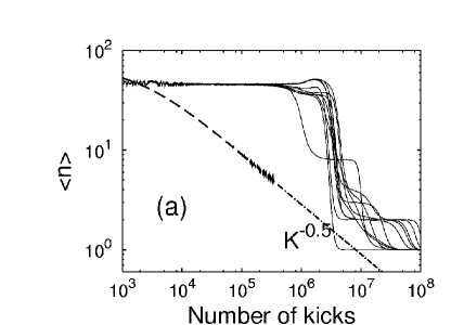
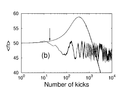
Figure 2: Mean principal quantum number $\langle n\rangle$, Eq. (7), for the same parameters as Fig. 1, $\langle n\rangle_{\rm cl}$: dashed line; $\langle n\rangle_{\rm qm}$: solid lines. (a): Long-time behavior (of $\log\langle n\rangle$), the dashed-dotted line indicates a fit to a power-law, and (b): short-time behavior of $\langle n\rangle$. The arrow in (b) indicates an approximate localization time defined in Eq. (16).

The classical $P_{\rm sur}^{\rm cl}(K)$ is obtained by the classical trajectory Monte Carlo method (CTMC) with a micro-canonical ensemble to represent the initial state arbi ; ctmc . The classical phase space (for $\Delta p>0$) is fully chaotic without any tori left intact. We show an example for the survival probability in Fig. 1. The classical $P_{\rm sur}^{\rm cl}(K)$ for times larger than $K_{0}$ kicks decays algebraically hill ,

$$P_{\rm sur}^{\rm cl}(K)=(K/K_{0})^{-\alpha}$$ (6)

with $\alpha\approx 1.5$. Both the time $K_{0}$ and the factor $\alpha$ are only weakly dependent on the parameters of the field ($\nu_{0}$ and $\Delta p_{0}$). By contrast, the quantum survival probability $P_{\rm sur}^{\rm qm}(K)$ displays a very different and much more complex behavior. One intriguing feature is an extreme sensitivity to the driving frequency $\nu_{0}$, especially in the long-time limit (compare also to the results in e. g. cas87 ; buch98 ; fish ). The resulting fluctuations in the kicked atom will be studied below in more detail (see Sect. IV).

For characterization of quantum (de)localization it is useful to introduce another observable that describes the bound portion of the wave packet. Inspired by the relation $n=1/\sqrt{-2E}$ for bound states, we introduce a mean quantum number as

$$\langle n(K)\rangle=\langle\psi(KT)|P_{\rm bound}\;\frac{1}{\sqrt{-2H_{0}}}\;P_{\rm bound}|\psi(KT)\rangle/P_{\rm sur}(K)\;.$$ (7)

In this equation, the expectation value is calculated for the portion of the wavefunction residing in the bound subspace. Equation (7) characterizes the specific position of that part of the wavefunction that remains bound, in particular that remains localized or stabilized near the initial state (or initial torus). Indeed, $\langle n\rangle$ displays a characteristically different behavior classically $\langle n\rangle_{\rm cl}$ and quantum mechanically $\langle n\rangle_{\rm qm}$, both at short times (Fig. 2b) and long times (Fig. 2a). The sharp drop of $\langle n\rangle_{\rm qm}$ from $50$ to $1$ at $K\approx 10^{6}$ will be analyzed in Sect. III.3. The corresponding non-normalized distributions $P(n,t)$ whose mean values are given by $\langle n\rangle$ are depicted in Fig. 3. The quantum $P^{\rm qm}(n,t)$ remains well localized close to the initial state while the time evolution of $P^{\rm cl}(n,t)$ features a rapid increase of width in the energy distribution and a shift towards increasingly lower energies (i.e. smaller $n$).

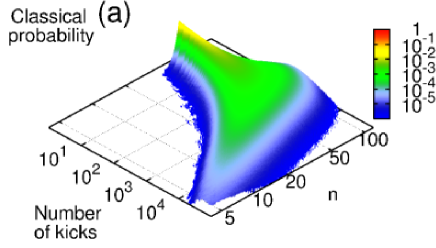
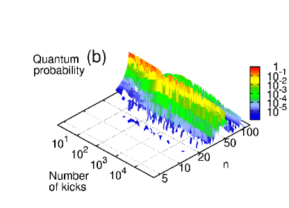
Figure 3: (Color online) Time-dependent spectral distribution $P(n,t)$, both classically (a) and quantum mechanically (b) for the same parameters as Fig. 2 (data shown for $\nu_{0}=1.45$).

Note, that classically $n$ does not possess a lower bound $n=1$, as the quantum distribution does. The fact that the energy distribution can grow to negative values without bound is at the root cause for the algebraic decay. The probability for crossing the $E=0$ line (i.e. the $n=\infty$ line) in the next time step and thus for reducing $P_{\rm sur}^{\rm cl}$ decreases as the mean distance to the $E=0$ line as measured by $\langle n(K)\rangle_{\rm cl}$ increases with $t$. We now relate the power-law decay Eq. (6) to the motion of $P^{\rm cl}(n,t)$ away from the threshold. The classical survival probability for large times is well fitted by Eq. (6) with $K_{0}\approx 1000$. The scaled average quantum-number is also well described by a power-law,

$$\langle n_{0}(K)~{}\rangle_{\rm cl}=b(K/K_{0})^{-0.5}\;,$$ (8)

where the power-law decay is assumed to start at the same time as that of the survival probability and $b\approx 1.8$. The differential form of Eq. (6),

$$\frac{dP_{\rm sur}^{\rm cl}(K)}{dK}=-\frac{\alpha}{K}P_{\rm sur}^{\rm cl}(K)\;,$$ (9)

can now be expressed by means of Eq. (8) as follows,

$$\frac{dP_{\rm sur}^{\rm cl}(K)}{dt}=-\frac{d}{K_{0}}\langle n_{0}(K)~{}\rangle_{\rm cl}^{2}P_{\rm sur}^{\rm cl}$$ (10)

with $d=\alpha/b^{2}$. For some cases with stronger average fields ($F_{0}^{\rm av}=0.02$ and $0.05$) shown in Figs. 4 and 5 (where $K_{0}\approx 60$ and $9$, respectively) we find that the power-law for $\langle n_{0}\rangle_{\rm cl}$, Eq. (8), holds with approximately the same constant $b$. Hence, Eq. (10) is still applicable and the constant $d$ has essentially the same value.

Figure 4: $\langle n\rangle$ averaged over the interval $1.45\leq\nu_{0}\leq 1.47$. In (a), $n_{i}=50$ and in (b), $|F_{0}^{\rm av}|=0.02$. Full line: quantum result and dashed line: classical result. The arrows indicate the lifetimes of the ground state estimated by direct coupling to the continuum. The average is calculated on the logarithmic scale, i.e. shown is $10^{<\log_{10}n>}$.

Figure 5: $P_{\rm sur}$ averaged over the interval $1.45\leq\nu_{0}\leq 1.47$. In (a), $n_{i}=50$, in (b), $|F_{0}^{\rm av}|=0.02$. Full line: quantum result, dashed line: classical result and dashed-dotted line: fit of classical result to a power-law. The arrows indicate the lifetimes of the ground state estimated by direct coupling to the continuum. The average is calculated on the logarithmic scale.

We now compare the numerical signatures of quantum localization for intermediary times as seen in $P_{\rm sur}$, Figs. 1a and 5, to the signatures seen in $\langle n\rangle$, Figs. 2a and 4. In all cases studied, the $\langle n\rangle^{\rm qm}>\langle n\rangle^{\rm cl}$ and a clear discrepancy between the quantum and the classical value can be seen for weak fields and low $n_{i}$. The discrepancy decreases as $|F_{0}^{\rm av}|$ or $n_{i}$ increases, i.e. $\langle n\rangle^{\rm qm}$ approaches the classical limit, however quite slowly. The approach to the classical limit appears faster in $P_{\rm sur}$. Here signatures of quantum localization can only be see for weak fields and low $n_{i}$ while in the other cases shown, $P_{\rm sur}^{\rm qm}$ has already reached the classical limit. We thus conclude that the more locally focused $\langle n\rangle$ provides stronger signature of quantum localization, i.e. the suppression of diffusion away from the initial state, than the $P_{\rm sur}$ probing the entire bound part of phase space.

III.2 Short-time dynamics: the cross-over to quantum localization

We take now a closer look at the short time dynamics for the weak field strength, Fig. 1b and Fig. 2b. Here a first surprise appears. One would, generally, expect $P_{\rm sur}^{\rm cl}$ and $P_{\rm sur}^{\rm qm}$ to agree with each other up to the localization time (or quantum break time, also referred to as Ehrenfest time) $\tau_{l}$. The present case is non-generic in that the classical phase space distribution remains up to $\tau_{l}$ ($\approx 200$ kicks) more localized when one identifies $P_{\rm sur}$ as a measure for localization. This quantum enhancement of ionization takes place even though the classical $\langle n\rangle_{\rm cl}$ moves closer to the ionization threshold while the quantum $\langle n\rangle_{\rm qm}$ remains close to the initial vale (Fig. 2b). The origin is a true quantum effect: perturbative single photon absorption of high frequency $m\nu_{0}$ from higher-harmonic components with $m\geq m_{c}(n_{i})$ sufficient to reach the continuum. Here

$$m_{c}(n_{i})=n_{i}/(2\nu_{0})\;.$$ (11)

A border for the field strength at which a single kick driving a high-lying Rydberg state displays quantum-classical correspondence can be found as follows jbhcp : The average classical energy transfer from a kick is

$$\Delta E_{k}=\Delta p_{0}^{2}\;.$$ (12)

This energy transfer can be resolved quantum mechanically if $\Delta E_{k}$ is not smaller than the quantum energy spacing $\Delta E_{n_{i}}^{0}=1/{n_{i}}$, leading to the critical momentum transfer

$$\Delta p_{0}^{\rm crit}=1/\sqrt{n_{i}}.$$ (13)

For $\Delta p_{0}>\Delta p_{0}^{\rm crit}$, the quantum and classical distributions after a single kick agree all the way up to the threshold $E=0$ since the quantum level spacing decreases as $n\to\infty$, and a good agreement between the quantum and classical survival probabilities is achieved. The difference between the classical and quantum distributions for $\Delta p_{0}<\Delta p_{0}^{\rm crit}$ can be understood by considering the dipole limit $\Delta p_{0}<\Delta p_{0}^{\rm dipole}=1/n_{i}$, for which the transition operator for a single kick, $\exp(i\Delta p\;q)$, reduces to

$$\exp\left(i\Delta p\;q\right)\approx 1+i\Delta p_{0}q_{0}n_{i}+...\;.$$ (14)

In this limit, the quantum transition amplitude is proportional to $\Delta p$ and the probability is proportional to $\Delta p^{2}$. By contrast, the classical probability is proportional to $\Delta p^{5}$ implying that the quantum survival probability after one kick is smaller than the classical one jbhcp . Physically, this can be understood by considering the Fourier transform of a delta kick,

$$\delta(t-t_{0})=\frac{1}{2\pi}\int\limits_{\infty}^{\infty}d\omega\exp\left(i\omega(t-t_{0})\right)\;,$$ (15)

indicating a “white” spectrum. The quantum system can absorb (virtual) photons of arbitrarily high frequency from the white spectrum accompanied by only a small momentum transfer $\Delta p_{0}\ll 1$. Processes with large energy transfer $\Delta\omega_{0}\gg 1$ but small momentum transfer $\Delta p_{0}$ are far from the line $\Delta\omega_{0}\approx\Delta p_{0}^{2}/2$ in the $\Delta\omega_{0}\;-\;\Delta p_{0}$ dispersion plane for a quasi-free electron, and thus effectively is inaccessible for a classical momentum transfer process. Only for deeply bound electrons with large local orbital momentum, $p_{0}$, near the nucleus, with $\Delta\omega_{0}\approx p_{0}\Delta p_{0}\gg\Delta p_{0}^{2}/2$ can such processes occur in the classical case. The density of classical phase space points for the initial state with such high $p_{0}$ is, however, very small. In the quantum case, the high-frequency components in the driving field interact non-locally with the whole initial state leading to an enhanced ionization probability. This corresponds to dipole allowed transitions. Classical-quantum correspondence is only restored when classical diffusion in phase space dominates the quantum enhancement due to (virtual) photon absorption.

Figure 6: As Fig. 1b, however for (a): $|F_{0}^{\rm av}|=0.02$ and $n_{i}=50$, (b): $|F_{0}^{\rm av}|=0.05$ and $n_{i}=50$, and (c): $|F_{0}^{\rm av}|=0.02$ and $n_{i}=200$.

For $n_{i}=50$ and $\nu_{0}=1.45$ the corresponding critical fields are $|F_{0}^{\rm crit}|=0.033$ and $|F_{0}^{\rm dipole}|=0.0047$, i.e. the case studied in Figs. 1 and 2 are close to the dipole limit. The important point is that the dynamical role of the high-harmonics spectrum of (virtual) photons is responsible for the surprising, non-generic features of the periodically kicked Rydberg atom, different from other systems such as the Rydberg atom in a microwave field. This is directly verified by increasing the field such that the scaled momentum transfer $\Delta p_{0}\approx\Delta p_{0}^{\rm crit}$, see Fig. 6. We show first a case in the transition region ($|F_{0}^{\rm av}|=0.02$, $n_{i}=50$) where still some traces of the non-generic features at short times can still be seen. For larger $n_{i}$ or larger $|F_{0}^{\rm av}|$ such that $\Delta p_{0}>\Delta p_{0}^{\rm crit}$ the quantum-classical agreement for short times is quite well fulfilled while discordance is found only for larger times, $t>\tau_{l}$. The short-time dynamics now conforms with the naive expectation of close classical-quantum correspondence for all $t<\tau_{l}$.

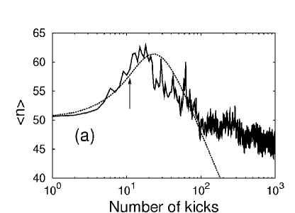
Figure 7: As Fig. 2b, however for (a): $|F_{0}^{\rm av}|=0.02$ and $n_{i}=50$, (b): $|F_{0}^{\rm av}|=0.05$ and $n_{i}=50$, and (c): $|F_{0}^{\rm av}|=0.02$ and $n_{i}=200$. The arrows indicate an approximate localization time defined in Eq. (16).

Well-known arguments aleiner for the localization time lead to the order of magnitude estimate

$$\tau_{l}\approx\frac{1}{\langle L\rangle}\;\ln\left(\frac{\langle q\rangle}{\lambda_{i}}\right)\;\;,$$ (16)

where $\langle q\rangle=n_{i}^{2}$ is the typical spatial extension of the initial state, $\lambda_{i}=n_{i}$ the wave length of the initial state, and $\langle L\rangle$ the mean Lyaponov exponent. $\tau_{l}$ is indicated by arrows in Fig. 2b and Fig. 7. For $\langle n\rangle$, $\tau_{l}$ gives a reasonable estimate for the number of kicks up to where quantum and classical dynamics mirror each other.

The situation for the survival probability is more involved: For $\Delta p_{0}<\Delta p_{0}^{\rm crit}$, Eq. (13) (see Figs. 1 and 6a), no agreement between $P_{\rm sur}^{\rm cl}$ and $P_{\rm sur}^{\rm qm}$ is found for short times and a break time $\tau_{l}$ now defined as the time where $P_{\rm sur}^{\rm cl}$ gets smaller than $P_{\rm sur}^{\rm qm}$ due to quantum localization takes on a different meaning. Consequently, this break time is not well described by Eq. (16). For the cases with $\Delta p_{0}>\Delta p_{0}^{\rm crit}$, (Figs. 5 and 6b and c) we find no clear numerical signatures of localization in $P_{\rm sur}$.

III.3 Long-time dynamics: the second cross-over

Quantum localization in the kicked Rydberg atom is transient. After a large but finite number of kicks (Figs. 1b and 6), the quantum survival probability rapidly decreases and at a second cross-over time (delocalization time) $\tau_{D}$ falls below even the classical value. Simultaneously, $\langle n\rangle_{\rm qm}$ drops sharply from values near $n_{i}$ to 1 (Figs. 2b and 7b). Beyond the cross-over point, $\langle n\rangle_{\rm cl}$ falls to values well below unity inaccessible to quantum mechanics. There, the residual fraction of the classical phase is “sheltered” and continues to decay slowly, i.e. algebraically. By contrast, the quantum bound-state probability decays exponentially in the long-time limit. Beyond $\tau_{D}$ the slow classical algebraic decay “wins” over the exponential decay. This novel scenario is markedly different from the sinusoidal driven Rydberg atom, where the quantum transport is bounded from below because of the regular phase space region, or, in a quantum picture, because of vanishingly small transition probabilities to states with low principal quantum numbers cas87 ; koch ; saw02 .

The rate of the long-time decay and, thus, of $\tau_{D}$ can be estimated from the decay rate of the state $n=1$ due to the high harmonics. This is the lowest-lying and most stable component of any coherent superposition forming a Floquet state. All frequencies of the driving field Eq. (3) with scaled energy $m\nu_{0}$ large enough to couple the Stark state having the largest overlap with the $n=1$ hydrogenic state to the Stark continuum contribute to the transition probability according to Fermi’s golden rule,

$$\Gamma_{m}=2\pi\rho(E_{m})|F^{\rm av}z(n=1,E_{m})|^{2}\;.$$ (17)

with $E_{m}=-1/2+m\nu_{0}/n_{i}^{3}$. Both dipole matrix elements $z(n,E)$ and the density of continuum states $\rho(E)$ are numerically obtained by diagonalizing the Stark Hamiltonian (2) in the pseudo-spectral basis. Summing over all contributions leads to a delocalization time $\tau_{D}=\left(\sum_{m}\Gamma_{m}\right)^{-1}$ which corresponds to within a factor of two to the lifetime of the most long-lived Floquet state with $\langle n\rangle\approx 1$. $\langle n\rangle_{\rm qm}$ averaged over an interval in $\nu$ ($1.45\leq\nu_{0}\leq 1.47$) together with the estimated $\tau_{D}$ are shown in Fig. 4. $\tau_{D}$ clearly gives a good estimate of the time-scale on which the break-down of quantum localization as seen in $\langle n\rangle$ takes place. The estimated $\tau_{D}$ also coincide with $P_{\rm sur}^{\rm qm}$ getting smaller than the classical value (Fig. 5). We thus attribute the break-down of quantum-localization to the higher harmonics in the driving field. The breakdown of localization is expected if the ground state $n=1$ is directly coupled to the continuum. We note parenthetically that an experimental realization would require half-cycle pulses with high-frequency components in the UV region. Work is currently under way on a protocol to produce half-cycle pulses in the atto-second regime atto .

We now comment on the decay of the quantum survival probability for $|F_{0}^{\rm av}|=0.005$ and $0.02$, $n_{i}=50$, seen for intermediate times ($K<10^{6}$ and $10^{4}$ in Figs. 5a and b, respectively). Here $\langle n\rangle^{\rm qm}\approx n_{i}$ (Fig. 4) indicating the localization of the quantum distribution $P(n,t)^{\rm qm}$ (see also Fig. 3b). As for $\langle n\rangle$, Eq. (7), we attribute the decay of the localized bound-part of the quantum wavefunction in the kicked atom to the higher harmonics present in the driving field, directly coupling the wave packet localized close to the initial state with the continuum.

IV Fluctuations in the survival probability

The quantum survival probability shown in Fig. 1 display strong fluctuations under small variations of the kick frequency. Such fluctuations are a direct consequence of the photonic localization scenario cas87 ; buch98 ; jensen , to be described in the following.

IV.1 High harmonics in the localization regime

The observation of localization, i.e. the suppression of ionization, or, equivalently, the freezing out of portions of the wavefunction near $n_{i}$, raises the question as to the underlying mechanism in the presence of the harmonic spectrum (Eq. (3) ). High harmonics cannot only directly couple to the continuum, see Sect. III.3, but they also can lead to sequential excitation through a ladder of intermediate (quasi)bound states. This channel is the dominant mechanism for the excitation and ionization by the harmonic driving by the lowest harmonic $\nu_{0}$. Jensen et al. jensen have discussed the suppression of the sequential ladder excitation by an harmonic driving as a mechanism for localization (“photonic localization”). It is therefore instructive to extend this approach to the present multi-photon case.

Following jensen we assume quasi-resonant one-photon transitions to dominate the time evolution, i.e. we consider only transition between (bound) states with energy differences to the initial state approximately equal to $k$ times the fundamental photon energy $E_{0}^{\gamma}=\nu_{0}/n_{i}$. The detunings

$$\Delta_{k}=E_{k}-E_{n_{i}}-k\nu$$ (18)

for the quasi-resonant states $\mid k\rangle$ form a pseudo-random sequence of numbers. Using the rotating wave approximation and setting $c_{k}(t)=b_{k}(t)\exp(-i\Delta_{k}t)$, with $b_{k}(t)$ the expansion coefficient for the ${\rm k^{th}}$ quasi-resonant state in the interaction picture, leads to a set of coupled differential equations,

$$i\frac{dc_{k}}{dt}=\sum\limits_{k^{\prime}}H^{J}_{kk^{\prime}}c_{k^{\prime}}$$ (19)

with the matrix $H^{J}$ given by

$$H^{J}_{kk^{\prime}}=\Delta_{k}\,\delta_{kk^{\prime}}+V_{k,k^{\prime}}.$$ (20)

The semiclassical expression for the coupling matrix elements is jensen

$$V_{kk^{\prime}}\approx 0.411F/\left((n_{k}\,n_{k^{\prime}})^{3/2}(m\nu_{0})^{5/3}\right)$$ (21)

with $m=|k-k^{\prime}|$ and $n_{k}$ the main quantum number of the ${\rm k^{th}}$ quasi-resonant state. While for the harmonically driven case $V_{kk^{\prime}}\neq 0$ only for $m=1$, the coupling matrix elements for the periodically kicked Rydberg atom in the ${\rm m^{th}}$ off diagonal are proportional to $m^{-5/3}$. Due to the randomness of the detunings $\Delta_{k}$, the matrix $H^{J}$ is thus a pseudo-random, power-law banded matrix. In random power-law banded matrices with the elements decreasing as $m^{-\beta}$, the eigenstates are (weakly) localized for $\beta\geq 1$ fyod . Our extension of the model introduced in jensen on the basis of cas87 thus predicts that the eigenstates for the kicked Rydberg atom should be localized. Infering from the numerical observation of quantum localization that the detunings are “sufficiently” random, the generalization of the photonic localization scenario appears applicable.

We finally comment on the (semi)classical border $n_{i}\to\infty$. Increasing $n_{i}$ from 50 to 200, the quantum localization for $|F_{0}^{\rm av}|=0.02$ almost vanishes (Figs. 4b and 5b). This indicates that a delocalization border is present in the kicked atom similar to that found for the harmonically driven system cas87 . The presence of a delocalization border implies a maximum $n_{i}$ for the applicability of the photonic localization theory. Detailed studies of this border in the kicked Rydberg atom remain to be performed.

IV.2 Characterization of parametric fluctuations

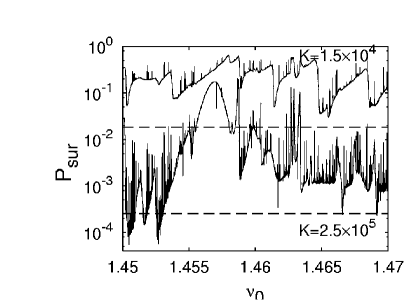
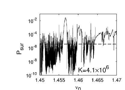
Figure 8: Survival-probability $P_{\rm sur}$ versus frequency $\nu$ for some numbers $K$ of kicks. $n_{i}=50$ and $|F_{0}|^{\rm av}=0.005$. The dashed lines give the classical results.

We turn now to a quantitative description of the parametric fluctuations of $P_{\rm sur}^{\rm qm}$ under variation of $\nu_{0}$ seen in Fig. 1. Fig. 8 displays the evolution towards an increasingly complex fluctuation pattern as $K$ increases. The amplitudes of the fluctuations increase by several orders of magnitude. Strong fluctuations in the survival probability have also been found e.g. in the harmonically driven Rydberg atom buch98 and in the kicked rotor when subjected to a varying Aharonov-Bohm flux casati01 or a variation of the kicking frequency sandro06 .

In order to characterize the increasingly finer scale on which these fluctuations occur, we determine the average distance between adjacent maxima and minima on the frequency scale, $\langle\delta_{\nu_{0}}(K)\rangle$. At times smaller than the delocalization time $\tau_{D}$, $\langle\delta_{\nu_{0}}(K)\rangle$ is rapidly decreasing (Fig. 9). A similar build-up of fluctuations in the survival probability with time is observed for the kicked rotor sandro06 . In the very-long time-limit beyond $\tau_{D}$, where the dynamics of the kicked system is governed by the decay of the ground state, no further fluctuations are produced but $\langle\delta_{\nu_{0}}(K)\rangle$ saturates.

Figure 9: Average distance $\langle\delta_{\nu_{0}}(K)\rangle$ between extrema in $P_{\rm sur}$ as a function of number $K$ of kicks. $n_{i}=50$ and $|F_{0}^{\rm av}|=0.005$. We analyze a set containing $10^{6}$ points on $1.45\leq\nu_{0}\leq 1.45008$.

It is now tempting to inquire whether the complexity of the fluctuations in the $P_{\rm sur}^{\rm qm}$ can be described by an approximate fractal dimension. For example, the fluctuations in the kicked rotor in the chaotic regime have been shown to have a fractal structure casati01 ; sandro06 . Fractal conductance fluctuations have been predicted ketz and experimentally found, e.g. hegger , for the transport through cavities with mixed classical phase space. A fractal structure has also been found in the survival probability of a system with a mixed phase space casati00 . In both cases, a semiclassical explanation based on on a classical power-law decay has been proposed. Since the kicked Rydberg atom displays classically such a power-law decay even though its phase space is fully chaotic, rather than mixed, a fractal is a conceivable candidate.

Figure 10: Fractal analysis of $\log_{10}(P_{\rm sur})$ for $n_{i}=50$ and $|F_{0}^{\rm av}|=0.005$. In (a) we show the data analyzed for $2\times 10^{6}$ points in the interval $1.45\leq\nu_{0}\leq 1.47$ for different numbers $K$ of kicks and in (b) we combine the wide set of (a) with data for a dense set containing $10^{6}$ points in the interval $1.45\leq\nu_{0}\leq 1.45008$ for $K=6.8\times 10^{7}$.

For a given “resolution” $\Delta\nu_{0}$ in frequency we calculate the local fractal dimension $D(\Delta\nu_{0})$ by means of a variational method varmeth . Rigorously, this value should be independent of $\Delta\nu_{0}$. In the present physical context, we are satisfied if $D(\Delta\nu_{0})$ is approximately constant over at least one order of magnitude in $\Delta\nu_{0}$. The fractal analysis of the data shown in Fig. 8 is presented in Fig. 10a. Since the survival probability fluctuates over many orders of magnitude, we analyze the logarithm of the data. After more than $10^{5}$ kicks, a plateau starts to develop, the width of which reaches almost two orders of magnitude for larger $K$. The value of $D$ on the plateau increases with $K$ up to about $D\approx 1.2$. The process of increasingly finer rescaling is transient and stops beyond $K>10^{7}$ when $\tau_{D}$ is reached. Zooming in on a narrow frequency interval for $K>K_{D}$, (Fig. 10b), the plateau value is still is $D\approx 1.2$, but the width of the plateau is only about one order of magnitude. Thus, a tendency towards a non-integer dimension can be found in the positively kicked Rydberg atom. The value is weakly dependent on the number $K$ of kicks for which the fractal analysis is made and appears to approach $D\approx 1.2$.

It is now instructing to compare this value with the semiclassical prediction ketz ; casati00 ; lai92 based on the power-law decay with exponent $\alpha=1.5$ (see Fig. 1) of the classical survival probability $P_{\rm sur}^{\rm cl}(K)$, $D_{\rm SC}=2-\alpha/2=1.25$. The value for $D_{\rm SC}$ is remarkably close to the plateau value found from the fractal dimension analysis. We thus conclude that the onset of a self-similar fluctuation pattern can be observed with a dimension close to the semiclassical prediction derived from the classical power-law decay. We note that this process is transient in that the finest scale for the fluctuations is determined by the time $\tau_{D}$ beyond which the most stable bound state decays.

V Summary

We have studied the long-time limit of quantum localization of the positively kicked Rydberg atom, involving clear signatures of a quantum suppression of classical ionization. We compare the localization as seen in the survival probability to that seen in an average quantum number $\langle n\rangle$ describing the position of the localized part of the wavefunction (see Eq. (7) ). In $\langle n\rangle$ clearer signatures of quantum localization prevailing to higher field strengths and larger quantum numbers are found. Two cross-over times could be identified. The cross-over from classical-quantum correspondence to localization ($\tau_{l}$) and the destruction or delocalization at a much later time ($\tau_{D}$). Remarkably, beyond $\tau_{D}$, the quantum system decays faster then the classical counterpart due to direct transitions to the continuum resembling photoionization. This process, identified in the present paper within a 1D model, is expected to be operative in a full 3D model as well. Quantum localization is accompanied by strong fluctuations in the survival probability after a given number of kicks as a function of the frequency of the driving field. The average distance between the fluctuations $\langle\delta_{\nu_{0}}(t)\rangle\propto 1/t$ until $t=\tau_{D}$, whereafter $\langle\delta_{\nu_{0}}\rangle$ saturates. In the localization regime, the complex fluctuation pattern approaches a fractal.

In this paper we have highlighted effects caused by the higher harmonics in the driving field distinguishing the kicked atom from the Rydberg atom driven by a microwave field. Further studies comparing these two systems, including an assessment on how closely the quantum localization in the kicked Rydberg atom is related to Anderson localization using e.g. the methods in cas87 ; buch98 , is left for forthcoming studies.

- (1) H.-J. Stöckmann, Quantum Chaos, an Introduction, Cambridge University Press (1999)
- (2) G. Casati, B. V. Chirikov, and D. L. Shepelyansky, Phys. Rep. 154, 77 (1987); G. Casati, I. Guarneri, and D. L. Shepelyansky , IEEE Jour. Quant. Elect. 24, 1420 (1988)
- (3) M. V. Berry, Physica D 33, 26 (1988)
- (4) G. Casati, B. V. Chirikov, F. M. Izraelev, and J. Ford, Lecture Notes in Phys. 93, 334 (Springer, 1979); G. Casati, I. Guarneri, and D. L. Shepelyansky, Phys. Rev. Lett. 62, 345 (1989)
- (5) S. Fishman, D. R. Grempel, and R. E. Prange, Phys. Rev. Lett. 49, 509 (1982)
- (6) S. Adachi, M. Toda, K. Ikeda, Phys. Rev. Lett. 61, 659 (1988)
- (7) F. L. Moore, J. C. Robinson, C. F. Bharucha, B. Sundaram, and M. G. Raizen, Phys. Rev. Lett. 75, 4598 (1995)
- (8) R. V. Jensen, S. M. Susskind, and M. M. Sanders, Phys. Rep 201, 1 (1991)
- (9) J. E. Bayfield and L. A. Pinnaduwage, Phys. Rev. Lett. 54, 313 (1985)
- (10) P. M. Koch and K. A. H. van Leeuwen, Phys. Rep. 255, 289 (1995)
- (11) A. Buchleitner, I. Guarneri, and J. Zakrzewski, Europhys. Lett 44, 162 (1998); S. Wimberger and A. Buchleitner, J. Phys. A 34, 7181 (2001)
- (12) A. Buchleitner, D. Delande, J. Zakrzewski, R. N. Mantegna, M. Arndt, and H. Walther, Phys. Rev. Lett. 75, 3818 (1995)
- (13) J. Leopold and D. Richards, J. Phys. B 22, 1931 (1989)
- (14) R. R Jones, D. You, and P. H. Bucksbaum, Phys. Rev. Lett. 70, 1236 (1993)
- (15) M. T. Frey, F. B. Dunning, C. O. Reinhold, J. Burgdörfer, Phys. Rev. A 53, R2929 (1996)
- (16) J. Bromage and C. R. Stroud, Phys. Rev. Lett. 83, 4963 (1999)
- (17) J. Burgdörfer, Nuc. Instr. Meth. B 42, 500 (1989); M. Melles, C. O. Reinhold, and J. Burgdörfer, ibid. 79, 109 (1993)
- (18) C. F. Hillermeier, R. Blümel, and U. Smilansky, Phys. Rev. A 45, 3486 (1992)
- (19) M. Klews and W. Schweizer, Phys. Rev. A 64, 053403 (2001)
- (20) J. Ahn, D. N. Hutchinson, C. Rangan, and P. H. Bucksbaum, Phys. Rev. Lett 86, 1179 (2001); T. J. Bensky, M. B. Campbell, R. R. Jones, Phys. Rev. Lett 81, 3112 (1998)
- (21) C. Wesdorp, F. Robicheaux, and L. D. Noordam, Phys. Rev. Lett 87, 083001 (2001)
- (22) S. Yoshida, C. O. Reinhold, and J. Burgdörfer, Phys. Rev. Lett. 84, 2602 (2000); S. Yoshida, C. O. Reinhold, P. Kristöfel, and J. Burgdörfer, Phys. Rev. A 62, 023408 (2000)
- (23) C. O. Reinhold, W. Zhao, J. C. Lancaster, F. B. Dunning, E. Persson, D. G. Arbó, S. Yoshida, and J. Burgdörfer, Phys. Rev. A 70, 033402 (2004)
- (24) E. Persson, S. Yoshida, X.-M. Tong, C. O. Reinhold, J. Burgdörfer, Phys. Rev. A 68, 063406 (2003)
- (25) X. M. Tong and S. I. Chu, Chem. Phys. 217, 119 (1997); J. Wang, Shih-I Chu, and C. Laughlin, Phys. Rev. A 50, 3208 (1994)
- (26) F. Borgonovi, I. Guarneri, L. Rebuzzini, Phys. Rev. Lett. 72, 1463 (1994)
- (27) R. Arbines and I. C. Percival, Proc. Phys. Soc. 88 861 (1966);
- (28) C. O. Reinhold, J. Burgdörfer, M. T. Frey, and F. B. Dunning, Phys. Rev. Lett. 79, 5226 (1997); M. T. Frey, F. B. Dunning, C. O. Reinhold, S. Yoshida, and J. Burgdörfer, Phys. Rev. A 59 1434 (1999)
- (29) C. O. Reinhold and J. Burgdörfer, J. Phys. B 26, 3101 (1993)
- (30) I. L. Aleiner and A. I. Larkin, Phys. Rev. B 54, 14423 (1996)
- (31) S. Wimberger, A. Krug, and A. Buchleitner, Phys. Rev. Lett 89, 263601 (2002)
- (32) E. Persson, K. Schissl, A. Scrinzi, and J. Burgdörfer, Phys. Rev. A (2006)
- (33) A. D. Mirlin, Y. V. Fyodorov, F.-M. Dittes, J. Quezada, and T. H. Seligman, Phys. Rev. E 54, 3221 (1996)
- (34) G. Benenti, G. Casati, I. Guarneri, and M. Terraneo, Phys. Rev. Lett. 87, 014101 (2001)
- (35) A. Tomadin, R. Mannella, and S. Wimberger, J. Phys. A 39, 2477 (2006)
- (36) R. Ketzmerick, Phys. Rev. B 54, 10841 (1996) ; A. S. Sachrajda, R. Ketzmerick, C. Gould, Y. Feng, P. J. Kelly, A. Delage, and Z. Wasilewski, Phys. Rev. Lett 80, 1948 (1998)
- (37) H. Hegger, B. Huckestein, K. Hecker, M Janssen, A. Freimuth, G. Reckziegel, and R. Tuzinski, Phys. Rev. Lett 77, 3885 (1996)
- (38) G. Casati, I. Guarneri, and G. Maspero, Phys. Rev. Lett. 84, 63 (2000)
- (39) B. Dubuc, J. F. Quiniou, C. Roques-Carmes, C. Tricot, and S. W. Zucker, Phys. Rev. A 39, 1500 (1989)
- (40) Y.-C. Lai, R. Blümel, E. Ott, and C. Grebogi, Phys. Rev. Lett 68, 3491 (1992)