Semiclassical Tunneling of Wavepackets with Real Trajectories

Abstract

Semiclassical approximations for tunneling processes usually involve complex trajectories or complex times. In this paper we use a previously derived approximation involving only real trajectories propagating in real time to describe the scattering of a Gaussian wavepacket by a finite square potential barrier. We show that the approximation describes both tunneling and interferences very accurately in the limit of small Planck’s constant. We use these results to estimate the tunneling time of the wavepacket and find that, for high energies, the barrier slows down the wavepacket but that it speeds it up at energies comparable to the barrier height.

I Introduction

The success of semiclassical approximations in molecular and atomic physics or theoretical chemistry is largely due to its capacity to reconcile the advantages of classical physics and quantum mechanics. It manages to retain important features which escape the classical methods, such as interference and tunneling, while providing an intuitive approach to quantum mechanical problems whose exact solution could be very difficult to find. Moreover, the study of semiclassical limit of quantum mechanics has a theoretical interest of its own, shedding light into the fuzzy boundary between the classical and quantum perspectives.

In this paper we will apply the semiclassical formalism to study the scattering of a one dimensional wavepacket by a finite potential barrier. In the case of plane waves, the tunneling and reflection coefficients can be easily calculated in the semiclassical limit, giving the well known WKB expressions merz . For wavepackets, however, the problem is more complicated and few works have addressed the question from a dynamical point of view Xav ; bez ; nov . The time evolution of a general wavefunction with initial condition $\psi(x,0)=\psi_{0}(x)$ can be written as

$$\psi(x,T)=<x|K(T)|\psi_{0}>= \int<x|K(T)|x_{i}>dx_{i}<x_{i}|\psi_{0}>,$$ (1)

where $K(T)=e^{-iHT/\hbar}$ is the evolution operator and $H$ is the (time independent) hamiltonian. The extra integration on the second equality reveals the Feynman propagator $<x|K(T)|x_{i}>$, whose semiclassical limit is known as the Van-Vleck formula  Va28 (see next section). When the Van-Vleck propagator is inserted in Eq.(1) we obtain a general semiclassical formula which involves the integration over the ‘initial points’ $x_{i}$:

$$\psi_{\textrm{sc}}(x,T)=\int<x|K(T)|x_{i}>_{\textrm{Van Vleck}}dx_{i}<x_{i}|\psi_{0}>.$$ (2)

If this integral is performed numerically one obtains very good results, specially as $\hbar$ goes to zero. However, doing the integral is more complicated than it might look, because for each $x_{i}$ one has to compute a full classical trajectory that starts at $x_{i}$ and ends at $x$ after a time $T$, which may not be simple task. Alternative methods involving integrals over initial conditions (instead of initial and final coordinates) in phase space have also been developed and shown to be very accurate kay97 ; BAKKS ; tanaka . All these approaches sum an infinite number of contributions and hide the important information of what classical trajectories really matter for the process.

In a previous paper Ag05 several further approximations for this integral were derived and applied to a number of problems such as the free particle, the hard wall, the quartic oscillator and the scattering by an attractive potential. The most accurate (and also the most complicated) of these approximations involves complex trajectories and was first obtained by Heller and collaborators Hu87 ; Hu88 . The least accurate (and the simplest to implement) is known as the Frozen Gaussian Approximation (FGA), and was also obtained by Heller He75 . It involves a single classical trajectory starting from the center of the wavepacket. However, other approximations involving real trajectories can be obtained Ag05 ; nov ; nov05 . These are usually not as accurate as the complex trajectory formula, but are much better than the FGA and can be very good in several situations. Moreover, it singles out real classical trajectories from the infinite set in Eq.(2) that can be directly interpreted as contributing to the propagation.

In this paper we apply these real trajectory approximations to study the tunnel effect. Since this is a purely quantum phenomena, it is a very interesting case to test the semiclassical approximation and to understand what are the real trajectories that contribute when the wavepacket is moving ‘inside’ the barrier. More specifically, we will consider the propagation of a Gaussian wavepacket through a finite square barrier. We shall see that the semiclassical results are very accurate, although some important features of the wavepacket propagation cannot be completely described.

This paper is organized as follows: in the next section we review the semiclassical results derived in Ag05 , which are the starting point of this work. Next we describe the evolution of a Gaussian through a square potential barrier in its three separate regions: before, inside and after the barrier. Finally in section IV we discuss the calculation of tunneling times, as proposed in Xav . We find that the barrier slows down the wavepacket at high energies, but that it speeds it up at energies comparable to the barrier height. Finally, in section V we present our conclusions.

II Approximation with complex and real trajectories

One important class of initial wavefunctions is that of coherent states, which are minimum uncertainty Gaussian wavepackets. In this paper we shall consider the initial wavepacket $|\psi_{0}>$ as the coherent state of a harmonic oscillator of mass $m$ and frequency $\omega$ defined by

$$|z\rangle=e^{-\frac{1}{2}|z|^{2}}e^{z\hat{a}^{{\dagger}}}|0\rangle,$$ (3)

where $|0\rangle$ is the harmonic oscillator ground state, $\hat{a}^{{\dagger}}$ is the creation operator and $z$ is the complex eigenvalue of the annihilation operator $\hat{a}$ with respect to the eigenfunction $|z\rangle$. Using the position and momentum operators, $\hat{q}$ and $\hat{p}$ respectively, we can write

$$\hat{a}^{{\dagger}}=\frac{1}{\sqrt{2}}\left(\frac{\hat{q}}{b}-i\frac{\hat{p}}{c}\right)\qquad z=\frac{1}{\sqrt{2}}\left(\frac{q}{b}+i\frac{p}{c}\right),$$ (4)

where $q$ and $p$ are real numbers. The parameters $b=(\hbar/m\omega)^{\frac{1}{2}}$ and $c=(\hbar m\omega)^{\frac{1}{2}}$ are the position and momentum scales respectively, and their product is $\hbar$.

In order to write the Van Vleck formula of the Feynman propagator, we need to introduce the tangent matrix. Let $S\equiv S(x_{f},T;x_{i},0)$ be the action of a classical trajectory in the phase space $(X,P)$, with $x_{i}=X(0)$ and $x_{f}=X(T)$. A small initial displacement $(\delta x_{i},\delta p_{i})$ modifies the whole trajectory and leads to another displacement $(\delta x_{f},\delta p_{f})$ at time $T$. In the linearized approximation, the tangent matrix $\mathfrak{M}$ connects these two vectors of the phase space

$$\begin{pmatrix}\dfrac{\delta x_{f}}{b}\\ \,\\ \dfrac{\delta p_{f}}{c}\end{pmatrix}=\begin{pmatrix}-\dfrac{S_{ii}}{S_{if}}&\quad-\dfrac{c}{b}\dfrac{1}{S_{if}}\\ \,&\,\\ \dfrac{b}{c}\left(S_{if}-S_{ff}\dfrac{S_{ii}}{S_{if}}\right)&\quad-\dfrac{S_{ff}}{S_{if}}\end{pmatrix}\begin{pmatrix}\dfrac{\delta x_{i}}{b}\\ \,\\ \dfrac{\delta p_{i}}{c}\end{pmatrix}\equiv\begin{pmatrix}m_{qq}&\;m_{qp}\\ \,&\,\\ m_{pq}&\;m_{pp}\end{pmatrix}\begin{pmatrix}\dfrac{\delta x_{i}}{b}\\ \,\\ \dfrac{\delta p_{i}}{c}\end{pmatrix}$$ (5)

where $S_{ii}\equiv\partial^{2}S/\partial x_{i}^{2},\,S_{if}\equiv\partial^{2}S/\partial x_{i}\partial x_{f}\equiv S_{fi}$ and $S_{ff}\equiv\partial^{2}S/\partial x_{f}^{2}$. In terms of the coefficients of the tangent matrix, the Van Vleck propagator is Va28

$$\langle x_{f}|K(T)|x_{i}\rangle_{VanVleck}=\frac{1}{b\sqrt{2\pi m_{qp}}}\exp\left[\frac{i}{\hbar}S(x_{f},T;x_{i},0)-i\frac{\pi}{4}\right].$$ (6)

For short times $m_{qp}$ is positive and the square root is well defined. For longer times $m_{qp}$ may become negative by going through zero. At these ‘focal points’ the Van Vleck formula diverges. However, sufficiently away from these points the approximation becomes good again, as long as one replaces $m_{qp}$ by its modulus and subtracts a phase $\pi/2$ for every focus encountered along the trajectory. We shall not write these so-called Morse phases explicitly.

Assuming some converging conditions, the stationary phase approximation allows us to perform the integral over $x_{i}$ in Eq. (2) (for more details, see  Ag05 ). We obtain

$$\psi(z,x_{f},T)_{sc}=\frac{b^{-1/2}\pi^{-1/4}}{\sqrt{m_{qq}+im_{qp}}}\exp\left[\frac{i}{\hbar}S(x_{f},T;x_{0},0)+\frac{i}{\hbar}p(x_{0}-q/2)-\frac{(x_{0}-q)^{2}}{2b^{2}}\right],$$ (7)

where $x_{0}$ is the value of the initial coordinate $x_{i}$ when the phase of the propagator is stationary. It is given by the relation

$$\frac{x_{0}}{b}+i\frac{p_{0}}{c}=\frac{q}{b}+i\frac{p}{c}\quad\text{where}\quad p_{0}=-\left(\frac{\partial S}{\partial x_{i}}\right)_{x_{0}}.$$ (8)

The end point of the trajectory is still given by $X(T)=x_{f}$. In spite of $q$ and $p$ being real, $x_{0}$ and $p_{0}$ are usually complex. This implies that the classical trajectories with initial position $x_{0}$ and momentum $p_{0}$ are complex as well, even with $x_{f}\in\mathbb{R}$. Eq. (7) was first obtained by Heller Hu87 ; Hu88 and it is not an initial value representation (IVR). There are a priori several complex trajectories satisfying the boundary conditions. Thanks to the stationary phase approximation, we were able to replace an integral over a continuum of real trajectories (2) by a finite number of complex ones (7). The problem is now solvable, but still quite difficult to compute. However, it turns out that, in many situations, these complex trajectories can be replaced by real ones, which are much easier to calculate Ag05 ; nov .

Therefore, we look for real trajectories that are as close as possible to the complex ones. Let $\left(X(t),P(t)\right)\in\mathbb{C}\times\mathbb{C}$ be the coordinates of a complex trajectory, and $\left(u(t),v(t)\right)$ a new set of variables defined by

$$u=\frac{1}{\sqrt{2}}\left(\frac{X}{b}+i\frac{P}{c}\right),\qquad v=\frac{1}{\sqrt{2}}\left(\frac{X}{b}-i\frac{P}{c}\right).$$ (9)

According to Eq. (8), the boundary conditions become

$$u(0)=\frac{1}{\sqrt{2}}\left(\frac{x_{0}}{b}+i\frac{p_{0}}{c}\right)=\frac{1}{\sqrt{2}}\left(\frac{q}{b}+i\frac{p}{c}\right)=z\quad\text{and}\quad X(T)=x_{f}.$$ (10)

The initial condition is then the complex coordinate $z$ and the final condition is the real position $x_{f}$. The real and imaginary parts of $z$ are related to the central position $q$ and the central momentum $p$ of the initial wavepacket respectively. This gives us three real parameters that we may use as boundary conditions to determine the real trajectory. But a particle whose initial conditions are $q$ and $p$ will not a priori reach $x_{f}$ after a time $T$. Although it is possible to satisfy such final condition, it will not usually happen because $X(T)$ is imposed by $q$ and $p$. Likewise, fixing the initial and final positions $q$ and $x_{f}$ will not generally lead to $P(0)=p$. Therefore we need to choose only two boundary conditions among the three parameters, and use the hamiltonian of the system to calculate analytically or numerically the third one. This means that the relation (8) will not be generally fulfilled and the hope is that it will be fulfilled approximately. For a discussion about the validity of this approximation, see the beginning of the third section in Ag05 . If we fix $(q,p)$, we obtain the Frozen Gaussian Approximation of Heller  He75 . This is an initial value representation that involves a single trajectory and is unable to describe interferences or tunneling, which are the aim of this paper. However, we can fix $X(0)=q\,,\,X(T)=x_{f}$ and calculate $P(0)=p_{i}$. When the complex quantities in Eq.(7) are expanded about this real trajectory we obtain Ag05

$$\psi(z,x_{f},T)_{sc}=\frac{b^{-1/2}\pi^{-1/4}}{\sqrt{m_{qq}+im_{qp}}}\exp\left[\frac{i}{\hbar}S(x_{f},T;q,0)+\frac{i}{2\hbar}pq-\frac{1}{2}\,\frac{im_{qp}}{m_{qq}+im_{qp}}\left(\dfrac{p-p_{i}}{c}\right)^{2}\right].$$ (11)

Eq. (11) is the semiclassical formula we are going to use in this paper. We shall show that, although still very simple, it can describe tunneling and interferences quite well.

III The 1-D square barrier

Consider the specific case of a particle of unit mass scattered by the 1-D square barrier defined by (see fig.1)

$$V(x)=\begin{cases}V_{0}&\text{if $x\in[-a,a]$ where $a\in\mathbb{R}^{+}$}\\ 0&\text{otherwise}\end{cases}.$$ (12)

The initial state of the particle is a coherent state $\psi(z,x,0)=\langle x|z\rangle$ with average position $q<-a$ and average momentum $p>0$, i.e., the wavepacket is at the left of the barrier and moves to the right. In all our numerical calculations we have fixed $V_{0}=0.5$ and defined the critical momentum $\tilde{p}=\sqrt{2V_{0}}=1$.

The application of the semiclassical formula Eq.11 requires the calculation of classical trajectories from q to $x_{f}$ in the time $T$. For the case of a potential barrier, the number of such trajectories depends on the final position $x_{f}$. This dependence, in turn, causes certain discontinuities in the semiclassical wavefunction.

Since the initial wavepacket starts from $q<-a$, it is clear that for $x_{f}>a$ (at the right side of the barrier) there is only one trajectory satisfying $x(0)=q$ and $x(T)=x_{f}$. This ’direct trajectory’ has $p_{i}>\sqrt{2V_{0}}$ and $x(t)$ increases monotonically from $q$ to $x_{f}$.

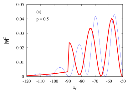
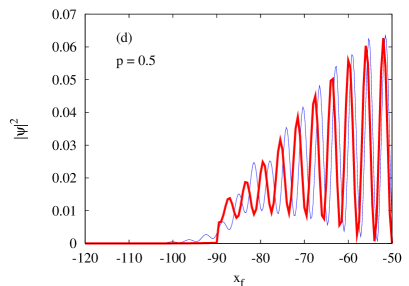
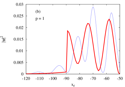
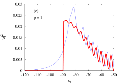
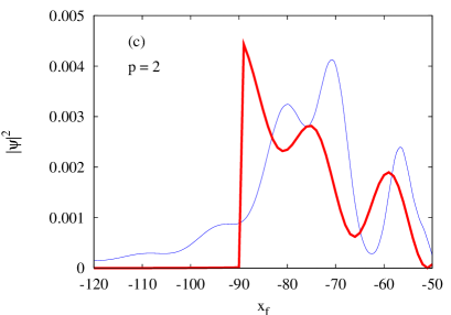
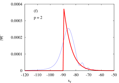
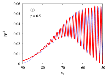
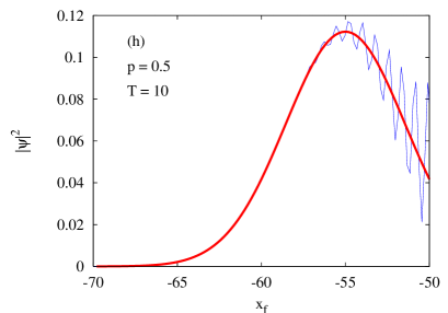
Figure 2: (Color online) Exact (blue thin lines) and semiclassical (red thick lines) wavepacket at time $T=50$, except for panel (h) where $T=10$. We fixed $\hbar=1$ for (a), (b) and (c), whereas $\hbar=1/4$ for (d), (e), (f), (h) and $\hbar=1/10$ for (g).

For $x_{f}<-a$, on the other hand, in addition to the direct trajectory there might also be a reflected trajectory, that passes through $x_{f}$, bounces off the barrier and returns to $x_{f}$ in the time $T$. The initial momentum of such a reflected trajectory must be greater than that of the direct one, since it has to travel a larger distance. However, if this distance is too big, i.e., if $x_{f}<<-a$, the initial momentum needed to traverse the distance in the fixed time $T$ becomes larger than $\sqrt{2V_{0}}$ and the reflected trajectory suddenly ceases to exist (see next subsection for explicit details for the case of the square barrier and figure 2 for examples).

This qualitative discussion shows that reflected trajectories exist only if $x_{f}$ is sufficiently close to the barrier. The points where these trajectories suddenly disappear represent discontinuities of the semiclassical calculation. Fortunatelly, this drawback of the approximation becomes less critical as $\hbar$ goes to zero, since the contribution of the reflected trajectory at those points become exponentially small as compared to the direct one (see for instance figure 2(g)).

In the remaining of this paper we are going to obtain explicit expressions for $\psi(z,x_{f},T)_{sc}$ before, inside and after the barrier. For fixed $q$ we will calculate the classical trajectories for each $x_{f}$, extracting the initial momentum $p_{i}$, the action $S\equiv S(x_{f},T;q,0)$ and its derivatives (in order to obtain $m_{qq}$ and $m_{qp}$).

III.1 Before the barrier: $x_{f}<-a$

The specificity of this region is that there may exist two different paths connecting $q$ to $x$ during the time $T$: a direct trajectory and a reflected one (fig. 1) whose initial momenta, action and tangent matrix elements are given by

$$p_{i\,d}=\frac{x-q}{T};\quad S_{d}=\frac{(x-q)^{2}}{2T};\quad m_{qq\,d}=1;\quad m_{qp\,d}=\frac{T}{\lambda},$$ (13)

$$p_{i\,r}=-\frac{x+q+2a}{T};\quad S_{r}=\frac{(x+q+2a)^{2}}{2T};\quad m_{qq\,r}=-1;\quad m_{qp\,r}=-\frac{T}{\lambda},$$ (14)

where $\lambda=b/c$. The contribution of each trajectory to the wavefunction at $x_{f}$, $\psi_{d}$ and $\psi_{r}$, is

$$\begin{array}[]{ll}\psi_{d}&=\frac{b^{-1/2}\pi^{-1/4}}{\sqrt{1+i\frac{T}{\lambda}}}\exp\left[\dfrac{i}{\hbar}\dfrac{(x_{f}-q)^{2}}{2T}+\dfrac{i}{2\hbar}pq-\dfrac{1}{2}\,\dfrac{iT}{\lambda+iT}\left(\dfrac{pT-x_{f}+q}{cT}\right)^{2}\right],\\ \\ \psi_{r}&=\frac{b^{-1/2}\pi^{-1/4}}{\sqrt{1+i\frac{T}{\lambda}}}\exp\left[i\theta+\dfrac{i}{\hbar}\dfrac{(x_{f}+q+2a)^{2}}{2T}+\dfrac{i}{2\hbar}pq-\dfrac{1}{2}\,\dfrac{iT}{\lambda+iT}\left(\dfrac{pT+x_{f}+q+2a}{cT}\right)^{2}\right].\end{array}$$ (15)

Notice that we have added an extra phase $\theta$ in $\psi_{r}$. Without this extra phase (that includes the minus sign coming from the tangent matrix elements in Eq.(14)), the wavepacket would not be continuous as it goes through the barrier. For a hard wall, for instance, we impose $\theta=\pi$ to guarantee that the wavefunction is zero at the wall. For smooth barriers this phase would come out of the approximation automatically, but for discontinuous potentials we need to add it by hand. To calculate $\theta$ we rewrite the previous expressions in complex polar representation, $\psi_{d}=D(x_{f})e^{i\varphi_{d}(x_{f})}$, $\psi_{r}=R(x_{f})e^{i\varphi_{r}(x_{f})+i\theta}$, and let $W(x_{f})e^{i\varphi_{w}(x_{f})+i\xi}$ be the wavefunction inside the barrier, where $\xi$ is the corresponding phase correction. The continuity of the wavefunction at $x_{f}=-a$ imposes

$$D(-a)e^{i\varphi_{d}(-a)}+R(-a)e^{i\varphi_{r}(-a)+i\theta}=W(-a)e^{i\varphi_{w}(-a)+i\xi}.$$ (16)

Eqs. (15) show that $R(-a)=D(-a)$ and $\varphi_{d}(-a)=\varphi_{r}(-a)$. Denoting $\varphi=\varphi_{w}(-a)-\varphi_{d}(-a)$, Eq. (16) becomes $1+e^{i\theta}=Ae^{i(\varphi+\xi)}$ where $A=[W(-a)/D(-a)]$. This complex relation represents in fact two real equations for the unknown variables $\theta$ and $\xi$. The solutions consistent with the boundary conditions are $\cos(\theta)=A^{2}/2-1$ and $\cos(\phi+\xi)=A/2$. In the limit where $p$ goes to zero (or the potential height $V_{0}$ goes to infinity) we obtain $\theta=\pi$ as expected. Finally, the full wavefunction before the barrier is $\psi(z,x_{f},T)_{sc}=\psi_{d}+\psi_{r}$ and the probability density can be written as

$$\begin{split}&|\psi(z,x_{f},T)_{sc}|^{2}=\frac{1}{b\sqrt{\pi}}\frac{1}{\sqrt{1+\frac{T^{2}}{\lambda^{2}}}}\Biggl{\{}\exp\left[-\frac{\lambda^{2}}{\lambda^{2}+T^{2}}\left(\dfrac{x_{f}-q-pT}{b}\right)^{2}\right]\\ &+\exp\left[-\frac{\lambda^{2}}{\lambda^{2}+T^{2}}\left(\dfrac{x_{f}+q+pT+2a}{b}\right)^{2}\right]\\ &+2\cos\left[\frac{2(x_{f}+a)}{\hbar(\lambda^{2}+T^{2})}\left(\lambda^{2}p-(q+a)T\right)-\theta\right]\exp\left[-\frac{\lambda^{2}}{\lambda^{2}+T^{2}}\dfrac{(pT+q+a)^{2}+(x_{f}+a)^{2}}{b^{2}}\right]\Biggr{\}}.\end{split}$$ (17)

This is the same result as obtained in Ag05 for a completely repulsive barrier ($V_{0}\rightarrow\infty$), except for the phase, because of the different boundary condition at $x_{f}=-a$ ($|\psi(-a)_{sc}|^{2}=0$ for the hard wall). However, as discussed in the beginning of this section, an additional difficulty appears when the wall is finite: the reflected trajectory does not always exist. From the classical point of view, there is no reflected part if the energy $E=p_{i\,r}^{2}/2>V_{0}$. The maximum initial momentum allowed is then $\sqrt{2V_{0}}$ and a particle with such momentum takes the time $T_{c}=-\dfrac{a+q}{\sqrt{2V_{0}}}$ to reach the barrier. Furthermore, for $T>T_{c}$ the reflected trajectory only exists if $p_{i\,r}=-\dfrac{x_{f}+q+2a}{T}\leqslant\sqrt{2V_{0}}$ i.e. if $|x_{f}|=-x_{f}\leqslant x_{c}=q+2a+\sqrt{2V_{0}}T$. Therefore, if $T\geqslant T_{c}$ and $|x_{f}|\leqslant x_{c}$, the probability density is given by Eq.(17), otherwise we only have the contribution of the direct $\psi_{d}$ and

$$|\psi(z,x_{f},T)_{sc}|^{2}=\frac{1}{b\sqrt{\pi}}\frac{1}{\sqrt{1+\frac{T^{2}}{\lambda^{2}}}}\exp\left[-\frac{\lambda^{2}}{\lambda^{2}+T^{2}}\left(\dfrac{x_{f}-q-pT}{b}\right)^{2}\right].$$ (18)

As a final remark we note that the calculation of $\theta$ might involve a technical difficulty depending on the values of $\hbar$, $p$ and $T$. For some values of these parameters the contribution of the direct and reflected trajectories might become very small at x=-a (see for instance fig.2(f), which shows the reflected wavepacket in a case of large transmission). In these cases the probability density becomes very small at x=-a and the value of the phase $\theta$ is irrelevant. In some of these situations, where the value of $\theta$ does not affect the results, we actually found that $\cos(theta)=A^{2}/2-1>1$, which cannot be solved for real $\theta$. For the sake of numerical calculations we have set $\theta=0$ in these cases.

The semiclassical wavepacket is now completely described for $x_{f}<-a$. The probability density $|\psi_{sc}|^{2}$ is a function of $q,p,x_{f},T$ and depends on several parameters, $a,b,\hbar$ and $V_{0}$. In our numerical calculations we fixed $a=50$. This makes the barrier large enough so that we study in detail what is happening inside (see subsection III.2). The height of the barrier intervenes only in $T_{c}$ and $x_{c}$ to establish the limits of the reflected trajectory. Its numerical value is not important, but its comparison with $p$ is fundamental: since we have fixed $V_{0}=0.5$ this gives $p_{i\,r}\leqslant\tilde{p}=\sqrt{2V_{0}}=1$. Finally, to simplify matters we fixed $b=c$, i.e. the same scale for position and momentum. This imposes $\lambda=b/c=1$. Quantum phenomena such as interference and tunneling should be more important for high values of $\hbar$. Since $\hbar=bc=b^{2}$, $b$ becomes in fact the only free parameter of the approximation. We have also fixed $q=-60$, which guarantees that the initial wavepacket is completely outside the barrier for all values of $b$ used.

Fig. 2 shows snapshots of the wavepacket as a function of $x_{f}$ at time $T=50$. Consider first the panels (a)-(c) with $\hbar=1$. The agreement between the exact and the semiclassical curves is qualitatively good for $p\leqslant\sqrt{2V_{0}}=1$. The interference peaks occurs at about the same positions, but the height of the peaks are not exactly the same. Also the intervals between peaks are a little bigger for the semiclassical curve than for the exact one. On the other hand, when $p$ is increased, the comparison gets worst and the approximation is not really accurate for $p=2$. However, we see that the value of $|\psi_{sc}|^{2}$ at $p=2$ is only a tenth of its value at $p=0.5$: the most important part of the wavepacket is in fact inside and after the barrier. It is then really important to consider $x_{f}>-a$ for high $p$ and we need to wait until subsections III.2 and III.3 to look at the whole picture.

When $\hbar=0.25$, Fig. 2(d)-(f) and (h), the approximation improves substantially, especially close to the barrier; this shows that the extra phase $\theta$ works well. When $p$ is increased, the contribution of the direct trajectory becomes irrelevant and the interference oscillations are lost in the semiclassical calculation, although it still shows good qualitative agreement in the average. The cut-off of the semiclassical curve at $x_{f}=-x_{c}$ is also clearly visible, whereas the exact one is decreasing continuously. On the one hand this means that the approximation is not perfect but, on the other hand, the semiclassical approximation explains that the fast rundown of the exact quantum wavepacket comes from the progressive disappearance of the reflected classical trajectory due to the finite size of the barrier. Finally, for $\hbar=0.1$, Fig. 2(g), the approximation becomes nearly perfect. As expected, the semiclassical approximation works better and better when $\hbar$ is decreasing, i.e. when the quantum rules give way to the classical ones.

To end this subsection, we mention that the quality of the approximation is independent of the time $T$, except for times slightly smaller than $T_{c}$. In this time interval only the direct trajectory contributes but the exact wavepacket already shows interferences that can not be described by $|\psi_{sc}|^{2}$ (fig. 2, $T=10$). We now enter the heart of the matter, and consider what’s happening inside and after the barrier.

III.2 Inside the barrier: $-a\leqslant x_{f}\leqslant a$

From the classical point of view there is only the direct trajectory in this region (see Fig. 1), since a reflection on the other side of the barrier (at $x=a$) can not be considered without quantum mechanics. Calling $p_{1}=p_{i}>\sqrt{2V_{0}}$ and $p_{2}$ the momentum of this trajectory before and inside the barrier respectively, energy conservation gives $p_{1}^{2}/2=p_{2}^{2}/2+V_{0}$. This is the first equation connecting $p_{1}$ to $p_{2}$, but we need a second one which is imposed by the propagation time $T=t_{1}+t_{2}$ where:

$\qquad t_{1}=-\frac{a+q}{p_{1}}$ is the time to go from $q$ to $-a$ with momentum $p_{1}$;

$\qquad t_{2}=\frac{x_{f}+a}{p_{2}}$ is the time to go from $-a$ to $x_{f}$ with momentum $p_{2}$.

The combination of these two equations gives

$$T=-\frac{a+q}{p_{1}}+\frac{x_{f}+a}{\sqrt{p_{1}^{2}-2V_{0}}}$$ (19)

which can be rewritten as

$$(p_{1}^{2}-2V_{0})(p_{1}T+a+q)^{2}=(x_{f}+a)^{2}p_{1}^{2}.$$ (20)

This is a quartic polynomial, which we solve numerically. We obtain four solutions: one is always negative, which we discard since we fixed the initial position $q$ on the left side of the barrier; two are sometimes complex and, when real, have $p_{1}<1$; finally, one of the roots is always real, larger than 1 and tends to $\frac{x_{f}-q}{T}$ when $V_{0}$ is negligible (the limit of a free particle). We take this last root as the initial momentum $p_{1}$.

The action $S$ is also a function of $p_{1}$ given by

$$\begin{split}S(z,x_{f},T)&=\int_{0}^{t_{1}}\frac{p_{1}^{2}}{2}\,dt+\int_{t_{1}}^{T}\left(\frac{p_{2}^{2}}{2}-V_{0}\right)\,dt\\ &=\frac{p_{1}^{2}}{2}\,t_{1}+\left(\frac{p_{2}^{2}}{2}-V_{0}\right)t_{2}\\ &=-\frac{1}{2}(a+q)p_{1}+\frac{1}{2}(x_{f}+a)\sqrt{p_{1}^{2}-2V_{0}}-\frac{V_{0}(x_{f}+a)}{\sqrt{p_{1}^{2}-2V_{0}}}.\end{split}$$ (21)

We calculate the derivatives of $S$ numerically by computing $p_{1}$ and $S$ for the initial conditions $(q,x_{f})$, $(q+dq,x_{f})$, $(q,x_{f}+dx_{f})$ …  and approximate $\dfrac{\partial S}{\partial x_{f}}(z,x_{f},T)$ by $[S(z,x_{f}+dx_{f},T)-S(z,x_{f},T)]/dx_{f}$, etc. Finally, the propagator inside the barrier is given by Eq.(11) plus the phase correction $\xi$ calculated in the previous subsection. The probability density, which in independent of $\xi$, becomes

$$|\psi(z,x_{f},T)_{sc}|^{2}=\frac{1}{b\sqrt{\pi}}\frac{1}{\sqrt{m_{qq}^{2}+m_{qp}^{2}}}\exp\left[-\frac{m_{qp}^{2}}{m_{qq}^{2}+m_{qp}^{2}}\left(\dfrac{p-p_{1}}{c}\right)^{2}\right].$$ (22)

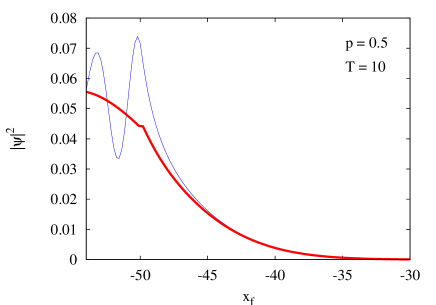
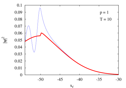
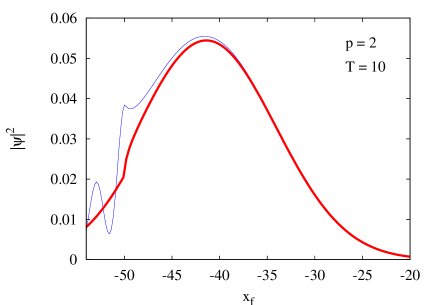
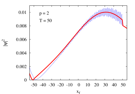
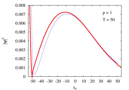
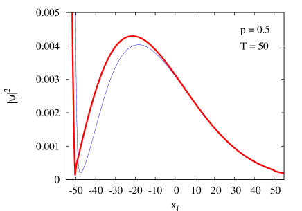
Figure 3: (Color online) Exact (blue thin lines) and semiclassical (red thick lines) wavepacket inside the barrier for various values of $p$ and $T$ and $\hbar=1$.

Figure 3 shows $|\psi_{sc}|^{2}$ as a function of $x_{f}$ for the same parameters as in subsection III.1. Although the semiclassical approximation also improves for small $\hbar$, here we shall fix $\hbar=1$. This is because the behavior of the propagator becomes trivial for small $\hbar$: if $p<1$ the wavepacket bounces off the barrier almost completely, and otherwise it simply passes over the barrier barely noticing the presence of the potential.

The first remark is that the wavepacket is continuous at $x_{f}=-a$: the extra phase $\theta$ does play its role correctly. As in the case before the barrier, the comparison between exact and semiclassical calculations is always at least qualitatively good, and sometimes even quantitatively so. However, there are two main effects that the semiclassical approximation cannot take into account.

1. there is a gap between the exact and semiclassical curves, which decreases progressively as $x_{f}$ increases, and is bridged near the local maximum of the probability density. The reason may come from the fact it is not possible to impose the continuity of the derivative of $\psi_{sc}$ with respect to $x_{f}$ at $-a$.

2. there are oscillations on the exact curve (especially for $p=2$ and $T=50$) close to the right side of the barrier, that are not present in the semiclassical approximation. This is a purely quantum effect, because classical mechanics can not account for a reflected trajectory which would interfere with the direct one in this case. $|\psi_{sc}|^{2}$ is in fact the mean-value of the oscillations, and that is why there is a discontinuity of the wavepacket at $x_{f}=a$, since the exact curve is beginning at the bottom of an oscillation.

If we want to stay strictly in the semiclassical limit, there is nothing we can do about the lack of interferences in the barrier region: this is the limit of our approximation. But if we want to use the semiclassical point of view in order to provide a more intuitive picture of the quantum world, we can add a ‘ghost’ trajectory that reflects at $x_{f}=a$ and see if it can account for the interferences. Similar ideas have been applied to the frequency spectrum of microwave cavities with sharp dielectric interfaces blumel and, more recently, to the spectrum of step potentials confined by hard walls koch . The argument will be the same as in subsection III.1, except of course that the reflected trajectory will now bounce on the right side of the barrier. The equation for $p_{i}=p_{1}$ is again a quartic polynomial given by

$$(p_{1}^{2}-2V_{0})(p_{1}T+a+q)^{2}=(3a-x_{f})^{2}p_{1}^{2}.$$ (23)

We know that $p_{1\,direct}$ is the same as $p_{1\,reflected}$ at $x_{f}=a$ and we choose the only solution of (23) which satifies this condition. The expression of the new action is:

$$S_{r}(z,x_{f},T)=-\frac{1}{2}(a+q)p_{1}+\left(\frac{p_{1}^{2}}{2}-2V_{0}\right)\frac{3a-x_{f}}{\sqrt{p_{1}^{2}-2V_{0}}}.$$ (24)

The expressions of $\psi_{d}$ and $\psi_{r}$ are the same as eq. (11) but with $p_{i},S,m_{qq}$ and $m_{qp}$ indexed by $d$ or $r$. After some calculations, the new expression of the probability density inside the barrier becomes

$$\begin{split}|\psi(z,x_{f},T)_{sc}|^{2}&=\frac{1}{b\sqrt{\pi}}\frac{1}{\sqrt{m_{qq\,d}^{2}+m_{qp\,d}^{2}}}\exp\left[-\frac{m_{qq\,d}^{2}}{m_{qq\,d}^{2}+m_{qp\,d}^{2}}\left(\frac{p-p_{1\,d}}{c}\right)^{2}\right]\\ &+\frac{1}{b\sqrt{\pi}}\frac{1}{\sqrt{m_{qq\,r}^{2}+m_{qp\,r}^{2}}}\exp\left[-\frac{m_{qq\,r}^{2}}{m_{qq\,r}^{2}+m_{qp\,r}^{2}}\left(\frac{p-p_{1\,r}}{c}\right)^{2}\right]\\ &+\frac{2}{b\sqrt{\pi}}\cos\left(\varphi_{r}-\varphi_{d}+\theta^{\prime}\right)\frac{1}{\sqrt[4]{\left(m_{qq\,r}^{2}+m_{qp\,r}^{2}\right)\left(m_{qq\,d}^{2}+m_{qp\,d}^{2}\right)}}\\ &\times\exp\left[-\frac{1}{2}\frac{m_{qq\,d}^{2}}{m_{qq\,d}^{2}+m_{qp\,d}^{2}}\left(\frac{p-p_{1\,d}}{c}\right)^{2}-\frac{1}{2}\frac{m_{qq\,r}^{2}}{m_{qq\,r}^{2}+m_{qp\,r}^{2}}\left(\frac{p-p_{1\,r}}{c}\right)^{2}\right],\\ \end{split}$$ (25)

where $\theta^{\prime}$ is the new extra phase (that absorbs the previously computed $\xi$) and

$$\begin{split}\varphi_{r}-\varphi_{d}=\frac{S_{r}-S_{d}}{\hbar}+\frac{1}{2}\arctan\left(\frac{m_{qp\,d}}{m_{qq\,d}}\right)-\frac{1}{2}\arctan\left(\frac{m_{qp\,r}}{m_{qq\,r}}\right)\\ +\frac{1}{2}\frac{m_{qq\,d}\,m_{qp\,d}}{m_{qq\,d}^{2}+m_{qp\,d}^{2}}\left(\frac{p-p_{1\,d}}{c}\right)^{2}-\frac{1}{2}\frac{m_{qq\,r}\,m_{qp\,r}}{m_{qq\,r}^{2}+m_{qp\,r}^{2}}\left(\frac{p-p_{1\,r}}{c}\right)^{2}.\end{split}$$ (26)

The results of such an expression, however, are not good: the oscillations become too big, which means that the reflected trajectory needs to be attenuated by a reflection coefficient $\rho$. To calculate $\rho$ we use the following reasoning: for each point $x_{f}$ inside the barrier there corresponds a reflected trajectory from $q$ to $x_{f}$ with a certain value of $p_{1}>1$ computed with Eq. (23). We take for $\rho$ the same attenuation coefficient a plane wave with momentum $p_{1}$ would have. Let $\left(F\,e^{i\kappa x_{f}}+G\,e^{-i\kappa x_{f}}\right)$ and $C\,e^{ikx_{f}}$ be such a plane wave inside and after the barrier respectively, where $\kappa=\sqrt{2(E-V_{0})}/\hbar=\sqrt{p_{1}^{2}-\tilde{p}^{2}}/\hbar$ and $k=\sqrt{2E}/\hbar=p_{1}/\hbar$. The continuity of this function and its derivative at $x_{f}=a$ give us the relative weight of the reflected trajectory with respect to the direct one:

$$\rho(p_{1},V_{0})=\left|\frac{G}{F}\right|=\frac{1-\kappa/k}{1+\kappa/k}=\frac{1-\sqrt{1-\tilde{p}^{2}/p_{1}^{2}}}{1+\sqrt{1-\tilde{p}^{2}/p_{1}^{2}}}.$$ (27)

The expression for the total propagator becomes $\left(\psi_{sc\,d}+\rho\,\psi_{sc\,r}\,e^{i\theta^{\prime}}\right)$. We use the same argument as in subsection III.1 to compute the extra phase $\theta^{\prime}$, adding another correction $\xi^{\prime}$ to the wavefunction on the right side of the barrier. Because there is always a single trajectory on the right side, $\xi^{\prime}$ does not affect the probability density there. We find that $\cos{\theta^{\prime}}=A_{+}^{2}/2-1$ where $A_{+}=W(a)/D(a)$.

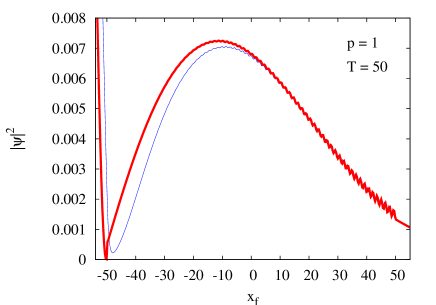
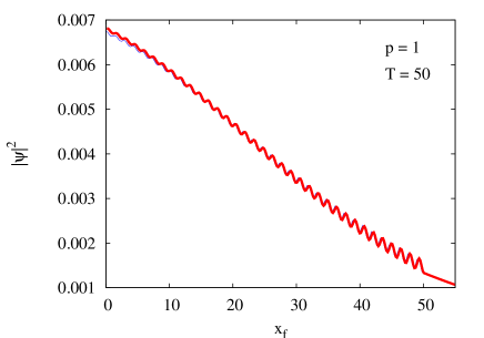
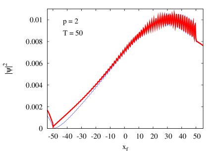
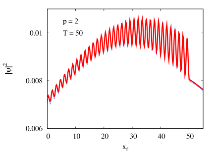
Figure 4: (Color online) Exact (blue thin lines) and semiclassical with ghost reflected trajectory (red thick lines) wavepacket inside the barrier . The panels on the right are magnifications of the left ones, showing the perfect match between the approximation and the exact solution.

The new results are displayed in figure 4. The gap is still present, but the agreement between exact and semiclassical on the right side is nearly perfect. The interferences are indeed coming from a real ’ghost’ trajectory that bounces off at the end of the barrier like a quantum plane wave. Since the left side of the figure has not changed much, the reflected trajectory has no effect on this part of the wavepacket and we don’t need to consider additional reflections. Furthermore, we don’t have to take $\rho\,\psi_{sc\,r}$ into account when we calculate $\theta$ in subsection III.1. We finish this subsection with two comments: first, the approximation with the ghost trajectory is accurate even for larger values of $\hbar$. Second, the wavepacket becomes continuous at $x_{f}=a$. That is very interesting because continuity comes only when we include the reflected trajectory, whereas the part of the wavepacket which goes through the barrier is calculated independently with a single direct trajectory (see next subsection). This means that the semiclassical propagator after the barrier somehow knows there is a reflected part.

In the next subsection, we will briefly present the computation of the wavefunction at the right side of the barrier.

III.3 After the barrier: $a<x$

Following the same arguments as in subsection III.2, we use the energy conservation $p_{1}^{2}/2=p_{2}^{2}/2+V_{0}=p_{3}^{2}/2$ (the index 3 refers to the right of the barrier) and the different times $t_{1}=-\frac{a+q}{p_{1}}$, $t_{2}=\frac{2a}{p_{2}}$ and $t_{3}=\frac{x-a}{p_{3}}$ to calculate the initial momentum of the direct trajectory. We obtain

$$(p_{1}^{2}-2V_{0})(p_{1}T+2a+q-x)^{2}=(2a)^{2}p_{1}^{2},$$ (28)

whereas the action becomes

$$\begin{split}S(z,x,T)&=\int_{0}^{t_{1}}\frac{p_{1}^{2}}{2}\,dt+\int_{t_{1}}^{t_{1}+t_{2}}\left(\frac{p_{2}^{2}}{2}-V_{0}\right)\,dt+\int_{t_{1}+t_{2}}^{T}\frac{p_{3}^{2}}{2}\,dt\\ &=\frac{1}{2}(x-q-2a)p_{1}+a\sqrt{p_{1}^{2}-2V_{0}}-\frac{2a\,V_{0}}{\sqrt{p_{1}^{2}-2V_{0}}}\end{split}.$$ (29)

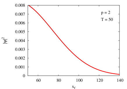
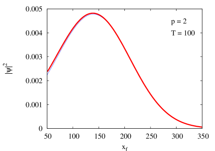
Figure 5: (Color online) Exact (blue thin lines) and semiclassical (red thick lines) wavepacket after the barrier for $p=2$ and $T=50$ and $100$.

In this region, no reflection is possible and the probability density $|\psi_{sc}|^{2}$ is simply given by Eq. (22). The results are presented in figure 5. For any values of $p$, $T$ or $\hbar$, there is still a very small difference between the exact and semiclassical curves for the ascending part of the wavepacket, whereas the agreement is perfect when the function is decreasing.

The conclusion of this section is that the semiclassical approximation with real trajectories gives very good results and is indeed able to describe some important quantum effects. Interference on the left side of the barrier appears naturally when the wavepacket hits the barrier and the comparison with the exact solution gets better as $\hbar$ gets smaller. However, these interferences cannot be obtained in the barrier region, since there are no reflected trajectories in the classical dynamics. We showed that these interferences can be recovered if a ‘ghost’ trajectory that reflects at $x=a$ is added and assumed to contribute with the same coefficient of a plane wave of initial momentum $p_{i}$. With this addition the semiclassical approximation becomes again very accurate inside the barrier. In the next section we shall briefly discuss the possibility of using our results to calculate the tunneling time as defined in Xav .

IV Semiclassical Tunneling Times

The question of how much time a particle spends in the classically forbidden region during the tunneling process has been attracting the attention of physicists for a long time hauge ; landauer ; Xav ; leavens ; ank ; cald ; cald2 ; xio . The very concept of a ‘tunneling time’ is, however, debatable leavens . Nevertheless, in a semiclassical formulation where real trajectories play crucial roles in the tunneling process, the temptation to estimate such a time is irresistible.

Since we are considering a wavepacket, and not a classical state localized by a point in the phase space, we can only define a mean value of the tunneling time. Let us fix the initial conditions $q,p$ (such that $p<1$) and $x_{f}>a$. The probability of finding the initial Gaussian state at $x_{f}$ after a time $T$ is given by $|<x_{f}|K(T)|z>|^{2}$. Therefore, the particle can reach $x_{f}$ from $(q,p)$ in several different time intervals $T$. For each value of the time $T$ there corresponds a single real trajectory whose initial momentum $p_{1}(T)>\tilde{p}=\sqrt{2V_{0}}$ is given by Eq. (28). This trajectory spends a time $\tau(T)=\frac{2a}{p_{2}(T)}=\frac{2a}{\sqrt{p_{1}^{2}(T)-\tilde{p}^{2}}}$ in the region $-a<x<a$. Notice that the average energy of the wavepacket is below the barrier but the contributing trajectory always has energy above the barrier. Therefore, for fixed $q,p,x_{f}$, the probability that the wavepacket crosses the barrier in a time $\tau(T)$ is proportional to $|<x_{f}|K(T)|z>|^{2}$. Following ref. Xav , we can define the mean value of the tunneling time as

$$\langle\tau\rangle=\mathfrak{N}^{-1}\int_{0}^{+\infty}\tau(T)\,|<x|K(T)|z>|^{2}\,dT$$ (30)

where

$$\mathfrak{N}=\int_{0}^{+\infty}|<x|K(T)|z>|^{2}\,dT$$ (31)

is the normalization factor. It is not equal to $1$ because only the part of the wavepacket which goes through the barrier is considered. This is important in our case, since the semiclassical approximation is better for $x_{f}>a$.

We calculated these integrals numerically, performing a discrete sum over $T_{n}=n\delta T$, with $n=1,2,\dots,N$ and $\delta T=T_{max}/N$. If an observer is placed at a fixed position $x_{f}>a$, as the time $T$ slips by, he/she sees the wavepacket arriving from the barrier, becoming bigger and bigger, reaching a maximum and then decreasing and disappearing. We ended the sum at $T_{max}$ such that $|<x|K(T)|z>|^{2}<10^{-4}\quad\forall~{}T>T_{max}$.

An important remark is that $\langle\tau\rangle$ is independent of the observer’s position $x_{f}$ (except for small fluctuations due to the numerical computation), since Eq.(30) measures only the time inside the barrier. The three different times we are going to use for comparison are:

• $\langle\tau_{barr}\rangle$ is the tunneling time computed according to Eq. (30)

• $\langle\tau_{free}\rangle$ is obtained from the same way as $\langle\tau_{barr}\rangle$, but in a system without barrier; $\langle\tau_{free}\rangle$ is simply the time for a free wavepacket to go from $-a$ to $a$.

• $\tau_{class}=\frac{2a}{\sqrt{p^{2}-\tilde{p}^{2}}}$ is the time required by a classical particle to cross the barrier.

Fig. 6 shows the dependence of these functions with respect to $p$. The curves become very similar as $p$ increases, because the barrier becomes more and more negligible. The wavepacket spreads but stays centered around $p$, which explains why it behaves like a particle of momentum $p$. When the influence of the barrier is more important, the wavepacket gets trapped by the barrier and slows down ($\langle\tau_{barr}\rangle$ is above $\langle\tau_{free}\rangle$), but for $p<1.8$, $\langle\tau_{free}\rangle$ and $\tau_{class}$ start to increase very fast ( $\tau_{class}$ actually diverges at $p=1$), whereas $\langle\tau_{barr}\rangle$ stays finite until $p$ is very close to $0$: thanks to the tunnel effect the wavepacket is accelerated by the barrier, which acts like a filter for the wavepacket and cuts off the contributions of its slowest components (see Fig. 7.(a)). On the other hand when $p$ increases, the fraction of the trajectories with $p<\sqrt{2V_{0}}=1$ becomes negligible and the barrier simply restrains the propagation of the wavepacket (fig. 7.(b)).

V Conclusion

In this paper we used the semiclassical approximation Eq. (11), derived in Ag05 , to study the propagation of a wavepacket through a finite square potential barrier. One of the main purposes of this work was to test the validity and accuracy of the approximation, which involves only real trajectories, in the description of tunneling. Surprisingly, we have shown that the approximation is very good to describe the wavepacket after the barrier, even when the average energy of the wavepacket is below the barrier height. The region before the barrier is also well described by the approximation, although discontinuities are always observed because of the sudden disappearance of the reflected trajectory. The continuity of the wavefunction between this region and the region inside the barrier also depends on the calculation of an extra phase $\theta$. Finally, inside the barrier the semiclassical formula is not able to describe interferences. These, however, can be recovered when a ghost trajectory, that reflects on the right side of the barrier, is included and attenuated with the proper coefficient. In all regions the approximation becomes more accurate as $\hbar$ becomes smaller.

The semiclassical approximation (11) is particularly relevant because the propagated wavepacket is not constrained to remain Gaussian at all times, as in the case of Heller’s Thawed Gaussian Approximation He75 , and also because it uses only a small number of real trajectories. These are much easier to calculate than complex ones, especially in multi-dimensional problems. The demonstration of its ability to describe tunneling and interferences is important to establish its generality and also to provide a more intuitive understanding the processes themselves. In particular, using the underlying classical picture, we have computed a tunneling time which shows that the wavepacket can be accelerated or restrained by the barrier depending on the value of the initial central momentum $p$.

Some interesting perspectives of this semiclassical theory are the study of propagations through smooth potential barriers (which are more realist and more adapted to semiclassical calculations), the study of time dependent barriers and the extension of the method to higher dimensions and to chaotic systems.

Acknowledgements

It is a pleasure to thank F. Parisio, A.D. Ribeiro and M. Novaes for many interesting comments and suggestions. This work was partly supported by the Brazilian agencies FAPESP, CNPq and FAEPEX.

Figure 1: Direct and reflected trajectories from $q$ to $x_{1}<-a$. For $-a<x_{2}<a$ or $x_{3}>a$ only the direct trajectory exists.

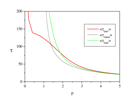
Figure 6: (Color online) Tunneling time as a function of $p$. The red thick line and the green curve show the semiclassical result according to Eq.(30) for the square barrier and the free particle respectively. The thin black line is the classical time for the square barrier potential.

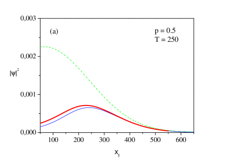
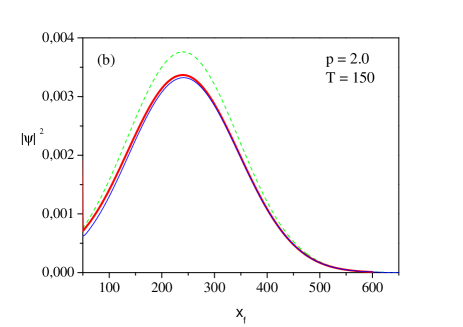
Figure 7: (Color online) Exact (blue thin lines) and semiclassical (red thick lines) wavepacket after going through the barrier. The green curve (above the other two in both figures) shows the corresponding free particle wavepacket. For $p=0.5$ the barrier acts like a filter and only the fast components of the initial wavepacket go through. For $p=2$, on the other hand, the wavepacket interacting with the barrier is slightly behind the free particle wavepacket, showing that the barrier slows the trajectories because the momentum is reduced to $p_{2}=\sqrt{p_{1}^{2}-2V_{0}}<p_{1}$ between $-a$ and $a$.

References

- (1) E. Merzbacher, Quantum Mechanics, cap. 7, 3rd edition, John Wiley and Sons, (1998).
- (2) A.L. Xavier Jr. and M.A.M. de Aguiar, Phys. Rev. Lett. 79, 3323 (1997).
- (3) F. Bezrukov and D. Levkov, J. Exp. Theor. Phys. 98, 820 (2004).
- (4) Marcel Novaes and M.A.M. de Aguiar, Phys. Rev. A 72, 32105 (2005).
- (5) J.H. Van Vleck, Proc. Nat. Acad. Sci. USA 14, 178 (1928).
- (6) Kenneth G. Kay, J. Chem. Phys. 107, 2313 (1997); Kenneth G. Kay, Ann. Rev. Phys. Chem. 56, 255 (2005).
- (7) M. Baranger, M.A.M. de Aguiar, F. Keck H.J. Korsch and B. Schellaas, J. Phys. A 34, 7227 (2001).
- (8) Atushi Tanaka, Phys. Rev. A 73, 24101 (2006).
- (9) M.A.M. de Aguiar, M. Baranger, L. Jaubert, F. Parisio, A.D. Riberio, J. Phys. A 38, 4645 (2005).
- (10) D. Huber, E.J. Heller, J. Chem. Phys. 87, 5302 (1987).
- (11) D. Huber, E.J. Heller, R.G. Littlejohn J. Chem. Phys. 89, 2003 (1988).
- (12) E.J. Heller, J. Chem. Phys. 62, 1544 (1975).
- (13) M. Novaes, J. Math. Phys. 46, 102102 (2005).
- (14) L. Sirko, P.M. Koch, and R. Blumel, Phys. Rev. Lett. 78, 2940 (1997).
- (15) A.S. Bhullar, R. Blümel and P.M. Koch, J. Phys. A: Math. Gen. 38, L563 (2005).
- (16) E. H. Hauge and J. A. Støvneng, Rev. Mod. Phys. 61, 917 (1989).
- (17) R. Landauer and Th. Martin, Rev. Mod. Phys. 66, 217 (1994).
- (18) C. R. Leavens, Found. Phys. 25, 229 (1995).
- (19) Joachim Ankerhold and Markus Saltzer, Phys. Lett. A 305, 251 (2002).
- (20) G. Garcia-Calderon and J. Villavicencio, Phys. Rev. A 66, 032104 (2002);
- (21) N. Yamada, G. Garcia-Calderon, and J. Villavicencio Phys. Rev. A 72, 012106 (2005).
- (22) Zhi-Yong Wang and Cai-Dong Xiong, quant-ph/0608031.