Measuring the size of a Schrödinger cat state

Abstract

We propose a measure for the ”size” of a Schrödinger cat state, i.e. a quantum superposition of two many-body states with (supposedly) macroscopically distinct properties, by counting how many single-particle operations are needed to map one state onto the other. This definition gives sensible results for simple, analytically tractable cases and is consistent with a previous definition restricted to Greenberger-Horne-Zeilinger-like states. We apply our measure to the experimentally relevant, nontrivial example of a superconducting three-junction flux qubit put into a superposition of left- and right-circulating supercurrent states and find this Schrödinger cat to be surprisingly small.

Introduction. - In his landmark 1935 paper Schrödinger (1935), Schrödinger introduced the notion of entanglement, and immediately pointed out its implications for measurement-like setups, where a microscopic quantum superposition may be transferred into a superposition of two “macroscopically distinct” states. His metaphor of a cat being in a superposition of “dead” and “alive”, initially designed just to reveal the bizarre nature of quantum mechanics, nowadays serves as a namesake and inspiration for a whole generation of experiments designed to test the potential limits of quantum mechanics in the direction of the transition to the “macroscopic” world, as well as to display the experimentalists’ prowess in developing applications requiring the production of fragile superpositions involving many particles. Recent experiments or proposals of this kind include systems as diverse as Rydberg atoms in microwave cavities Raimond et al. (2001), superconducting circuits Mooij et al. (1999); van der Wal et al. (2000); Friedman et al. (2000); Marquardt and Bruder (2001); Buisson and Hekking (2001); Vion et al. (2002), optomechanical Mancini et al. (1997); Marshall et al. (2003) and nanoelectromechanical Armour et al. (2002) systems, molecule interferometers Arndt et al. (1999), magnetic biomolecules Awschalom et al. (1992), and atom optical systems Julsgaard et al. (2001) (for a review with more references, see Ref. Leggett (2002)).

The obvious question of just how many particles are involved in such a superposition has not found any general answer so far Leggett (2002), and discussions of this point in relation to existing experiments have often remained qualitative. While the number of atoms participating in a macroscopic superposition of a $C_{60}$ molecule being at either one of two positions separated by more than its diameter is obviously sixty, the mere presence of a large number of particles in the system is not sufficient in itself. This is demonstrated clearly by the example of a single electron being shared by two atoms in a dimer, atop the background of a large number of “spectator electrons” in the atoms’ core shells. Therefore, obtaining a general measure for the “size” of a superposition of two many-body states is nontrivial, especially for systems such as superconducting circuits, where the relevant superimposed many-body states are not spatially separated.

Before proposing our solution to this challenge, we state right away that certainly more than one reasonable definition is conceivable, depending on which features of the state are deemed important for the superposition to be called “macroscopic”. Previous approaches can be roughly grouped into two classes: Measures of the first kind involve considering some judiciously chosen observable, evaluating the difference between its expectation values for the two superimposed states, and expressing the result in some appropriate “microscopic units” Leggett (1980, 2002) or in units of the spread of the individual wave packets Björk and Mana (2004). Several recent experiments have produced Schrödinger cats that, by those measures, are remarkably ”fat”. For example, for the experiments in Delftvan der Wal et al. (2000) and SUNYFriedman et al. (2000), the clock- and counterclockwise circulating supercurrents, whose superposition was studied, were in the micro-Ampere range, leading to a difference of $10^{6}\mu_{B}$ or even $10^{10}\mu_{B}$ in the magnetic moments, respectively.

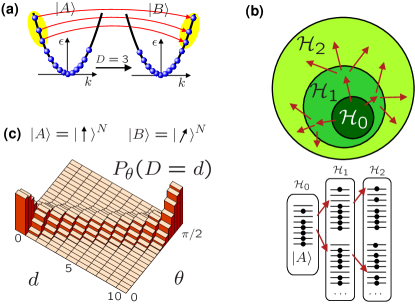
Figure 1: (Color online) (a) Example of normal-state persistent currents mentioned in the text, where $D=3$ single-particle operations are needed to turn state $\left|A\right\rangle$ into $\left|B\right\rangle$. (b) Hilbert spaces $\mathcal{H}_{d}$ generated by repeated application of single-particle operators. (c) Probability distribution $P_{\theta}(D=d)$ for the distance $D$ between two BEC states or between the two components of a generalized GHZ state, as a function of the angle between the corresponding single-particle states, for $N=10$ particles, see Eq. (4).

Measures of the second kind, in contrast, try to infer how many particles are effectively involved in those superpositions, which will be the focus of our paper. This category comprises Leggett’s “disconnectivity” Leggett (1980, 2002) and the measure of Dür, Simon and Cirac Dür et al. (2002) (DSC). The latter applies to a class of generalized Greenberger-Horne-Zeilinger (GHZ) states, which it compares to standard GHZ states in terms of susceptibility to decoherence and entanglement content.

In this paper, we propose a general definition for the size of a Schrödinger cat, or the effective distance between its two constituent many-body states, that is based on asking the following question: “How many single-particle operations are needed (on average) to map one of the two states to the other?” (see Fig. 1 a)

We will make this definition precise using the language of second quantization and show that in simple analytically tractable cases it agrees with reasonable expectations and with the measure of DSC Dür et al. (2002). After analyzing the general features of our measure, we evaluate it numerically for a superconducting three-junction flux qubit, whose eigenstates we find by exact numerical diagonalization. The resulting size turns out to be surprisingly small, which we attribute to the fact that repeated applications of single-particle operators quickly produce a very large Hilbert space, in which the “target” many-body state can be represented accurately.

Definition of the measure. - We start with a simple example. Consider a clean, ballistic, single-channel metallic ring capable of supporting normal-state persistent currents of electrons. Suppose it is put in a superposition of two Slater determinants, $\left|A\right\rangle$ and $\left|B\right\rangle$, which differ only in the number of right- and left-moving electrons (Fig. 1 a). The number of particles effectively participating in this superposition is clearly equal to the number of particles that have to be converted from right- to left-movers, in order to turn one of these many-body states into the other. This is identical to the number $D$ of single-particle operations that have to be applied to effect this change: $\left|B\right\rangle\propto\prod_{j=1}^{D}\hat{c}_{k^{\prime}_{j}}^{\dagger}\hat{c}_{k_{j}}\left|A\right\rangle$.

When turning this into a general definition, we have to realize that the “target” state $\left|B\right\rangle$ might be a superposition of components that can be created from $\left|A\right\rangle$ by applying different numbers $d$ of single-particle operations. In that case, we will end up with a probability distribution $P(D=d)$, defined as the weights of these components, for the “distance” $D$ between $\left|A\right\rangle$ and $\left|B\right\rangle$ to equal $d$. Furthermore, repeated application of single-particle operations may lead to a state that could have been created by a smaller number of such operations (such as $\left|B\right\rangle\propto\hat{c}_{k}^{\dagger}\hat{c}_{k^{\prime}}\hat{c}_{k^{\prime}}^{\dagger}\hat{c}_{k}\left|A\right\rangle\propto\left|A\right\rangle$ if $n_{k}=1$ and $n_{k^{\prime}}=0$). This has to be taken care of by projecting out the states that have been reached already.

The general definition (whether for fermions or bosons) is obtained by starting from the Hilbert space $\mathcal{H}_{0}\equiv{\rm span}\{\left|A\right\rangle\}$, and applying iteratively the following scheme, to generate spaces $\mathcal{H}_{1},\mathcal{H}_{2},\ldots$ (Fig. 1 b): Given a Hilbert space $\mathcal{H}_{d}$, apply all possible single-particle operators $\hat{c}_{j}^{\dagger}\hat{c}_{i}$ to all of its vectors. Consider the span of the resulting vectors and subtract the orthogonal projection on all previous Hilbert spaces, $\mathcal{H}_{0}\oplus\mathcal{H}_{1}\oplus\ldots\oplus\mathcal{H}_{d}$, thereby generating $\mathcal{H}_{d+1}$. This scheme is guaranteed to produce all vectors that can be generated from $\left|A\right\rangle$ by the time-evolution of an arbitrary (interacting, possibly time-dependent, but particle-conserving) Hamiltonian. Thus, we can represent the “target” state $\left|B\right\rangle$ (which is assumed to have the same particle number) as a superposition

$$\left|B\right\rangle=\sum_{d=0}^{\infty}\lambda_{d}\left|v_{d}\right\rangle$$ (1)

of orthonormalized vectors $\left|v_{d}\right\rangle\in\mathcal{H}_{d}$. The amplitudes $\lambda_{d}$ (defined up to a phase) produce the probability distribution for the distance $D$ from $\left|A\right\rangle$ to $\left|B\right\rangle$,

$$P(D=d)\equiv|\lambda_{d}|^{2}\,,$$ (2)

from which an average distance $\bar{D}$ may be obtained.

Generalized GHZ states. - Before discussing general features, let us consider an important example, namely a superposition of two non-interacting pure Bose condensates, $\left|A\right\rangle$ and $\left|B\right\rangle$, with $N$ particles being simultaneously in the single-particle state $\left|\alpha\right\rangle$ or $\left|\beta\right\rangle$, respectively, where $\left\langle\alpha\left|\beta\right.\right\rangle=\cos\theta$. We can write the two BEC many-body states as $\left|A\right\rangle=(N!)^{-1/2}(\hat{c}_{1}^{\dagger})^{N}\left|{\rm Vac}\right\rangle$ and $\left|B\right\rangle=(N!)^{-1/2}(\cos\theta\hat{c}_{1}^{\dagger}+\sin\theta\hat{c}_{2}^{\dagger})^{N}\left|{\rm Vac}\right\rangle$, with $\hat{c}_{1}^{\dagger}$ creating a particle in state $\left|\alpha\right\rangle$, and $\hat{c}_{2}^{\dagger}$ creating a particle in the state that defines the orthogonal direction in ${\rm span}\{\left|\alpha\right\rangle,\left|\beta\right\rangle\}$ (we have dropped a potentially present, but irrelevant global phase). Expanding $\left|B\right\rangle$, we find:

$$\left|B\right\rangle=\frac{1}{\sqrt{N!}}\sum_{d=0}^{N}\left(\begin{array}[]{c}N\\ d\end{array}\right)\left(\sin\theta\hat{c}_{2}^{\dagger}\right)^{d}\left(\cos\theta\hat{c}_{1}^{\dagger}\right)^{N-d}\left|{\rm Vac}\right\rangle.$$ (3)

Then $\left|v_{d}\right\rangle=[d!(N-d)!]^{-1/2}\left(\hat{c}_{2}^{\dagger}\right)^{d}\left(\hat{c}_{1}^{\dagger}\right)^{N-d}\left|{\rm Vac}\right\rangle$ is a normalized state that can be reached from $\left|A\right\rangle$ in exactly $d$ applications of the single-particle operator $\hat{c}_{2}^{\dagger}\hat{c}_{1}$, i.e. $\left|v_{d}\right\rangle\in\mathcal{H}_{d}$. Thus, $\left|B\right\rangle$ may be represented in the form (1), with coefficients

$$\lambda_{d}=\sqrt{\left(\begin{array}[]{c}N\\ d\end{array}\right)}\sin^{d}\theta\cos^{N-d}\theta.$$ (4)

The resulting distribution $P_{\theta}(D=d)=|\lambda_{d}|^{2}$ is binomial (Fig. 1 c), with probability $p=\sin^{2}\theta=1-|\left\langle\alpha\left|\beta\right.\right\rangle|^{2}$, and thus the average distance turns out to be $\bar{D}=Np$. It will be maximal, $\bar{D}=N$, for two orthogonal single-particle states, as expected. This example can be transcribed into spin-language, by considering the states $\left|A\right\rangle=\left|\uparrow\right\rangle^{N}$ and $\left|B\right\rangle=(\cos\theta\left|\uparrow\right\rangle+\sin\theta\left|\downarrow\right\rangle)^{N}$. In that case, we have to adapt our approach by defining single-spin operators as the single-particle operations, and replace $\hat{c}_{2}^{\dagger}\hat{c}_{1}$ by $\sum_{j=1}^{N}\hat{\sigma}_{-}^{(j)}$. Straightforward algebra shows the results for $P(D=d)$ and $\bar{D}$ to be the same. Comparing to DSC Dür et al. (2002), where such generalized GHZ-states were analyzed, we find that our result agrees precisely with theirs, for this special class of states, to which the analysis of DSC was restricted.

General features. - We can prove that the Hilbert spaces $\mathcal{H}_{d}$ thus constructed do not depend on the choice of the single-particle basis used to define the operators $\hat{c}_{i}^{\dagger}\hat{c}_{j}$. Consider an arbitrary unitary change of basis, $\hat{c}_{i}^{\prime}=\sum_{j}U_{ij}\hat{c}_{j}$. Starting from an arbitrary vector $\left|v\right\rangle$, we want to show that ${\rm span}\{\hat{c}_{i}^{\prime\dagger}\hat{c}_{j}^{\prime}\left|v\right\rangle\}={\rm span}\{\hat{c}{}_{i}^{\dagger}\hat{c}{}_{j}\left|v\right\rangle\}$ (where $i,j$ range over the basis). Indeed, any vector $\left|w\right\rangle$ from the Hilbert space on the left-hand-side can be written as $\left|w\right\rangle=\sum_{i^{\prime},j^{\prime},i,j}\mu_{i^{\prime},j^{\prime}}U_{i^{\prime}i}^{*}U_{j^{\prime}j}\hat{c}_{i}^{\dagger}\hat{c}_{j}\left|v\right\rangle$, which is an element of the right-hand-side (and vice versa). As a result, no particular basis (e.g. position) is singled out.

We can prove as well that the distance is symmetric under interchange of $\left|A\right\rangle$ and $\left|B\right\rangle$ for an important class of states, namely those connected by time-reversal (such as left- and right-going current states considered below). With respect to a position basis of real-valued wave functions, this means $\left|A\right\rangle=\left|B\right\rangle^{*}$. In that case, since the single-particle operators can be chosen real-valued, we have $\mathcal{H}_{d}^{A\rightarrow B}=(\mathcal{H}_{d}^{B\rightarrow A})^{*}$, making the weights $P^{A\rightarrow B}(D=d)$ and $P^{B\rightarrow A}(D=d)$ equal. The example treated above can also be expressed in this way, by an appropriate change of basis, with $\left|A/B\right\rangle\propto(\cos(\frac{\theta}{2})\hat{c}_{1}^{\dagger}\pm i\sin(\frac{\theta}{2})\hat{c}_{2}^{\dagger})^{N}\left|{\rm Vac}\right\rangle$. For other, non-symmetric pairs of states $\left|A\right\rangle$,$\left|B\right\rangle$, this is not true any longer, i.e $P^{A\rightarrow B}$ can become different from $P^{B\rightarrow A}$. An extreme example is provided by the states $\left|A\right\rangle=\frac{1}{\sqrt{2}}(\left|N,0\right\rangle+\left|0,N\right\rangle)$ and $\left|B\right\rangle=\left|N-1,1\right\rangle$, for $N$ bosons on two islands (with $\left|n_{1},n_{2}\right\rangle$ denoting the particle numbers). Here $P^{A\rightarrow B}(D=1)=1$, but $P^{B\rightarrow A}(D=1)<1$, with $P^{B\rightarrow A}(D=N-1)\neq 0$. In the following, we will restrict our discussion to time-reversed pairs of states.

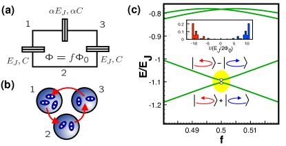
Figure 2: (Color online) (a) Circuit diagram of the three-junction flux qubit. (b) Equivalent representation in the charge basis. (c) Energy-level diagram for $E_{J}/E_{C}=20$ and $\alpha=1$, as a function of magnetic frustration. At $f=0.5$, the ground and first excited state are superpositions of left- and right-going current states, $\left|\pm I\right\rangle$, the states between which we calculate the “distance” $D$. The current distribution in the ground state is displayed in the inset.

Application to superconducting circuits. - A superconducting circuit such as a Cooper pair box or a flux qubit device can be viewed as a collection of metallic islands between which Cooper pairs are allowed to tunnel coherently through Josephson junctions. Adopting a bosonic description, we would describe tunneling by a term $\hat{c}_{i}^{\dagger}\hat{c}_{j}$, where $\hat{c}_{j}$ annihilates a Cooper pair on island $j$. However, as the total “background” number of Cooper pairs $\bar{n}$ on any island is very large and ultimately drops out of the calculation, the more convenient (and standard) approach is to consider instead operators $e^{-i\hat{\varphi}_{j}}=\sum_{n}\left|n-1\right\rangle_{j}\left\langle n\right|_{j}$ that reduce the number of Cooper pairs on island $j$ by exactly one. Then, the tunneling term becomes $\bar{n}^{-1}\hat{c}_{i}^{\dagger}\hat{c}_{j}\mapsto e^{i(\hat{\varphi}_{i}-\hat{\varphi}_{j})}$, while the total electrostatic energy may be expressed by the number operators $\hat{n}_{j}$ that count the number of excess Cooper pairs on each island. These two types of operators define the single-particle operators needed in our approach.

Let us now apply the measure defined above to a particular, experimentally relevant case, the three-junction flux qubit that has been developed in Delft Mooij et al. (1999); Orlando et al. (1999); van der Wal et al. (2000). Three superconducting islands are connected by tunnel junctions (Fig. 2), where the tunneling amplitude is given by the Josephson coupling $E_{J}$, and the charging energy $E_{C}=e^{2}/2C$ is determined by the capacitance $C$ of the junctions. One of the junctions is smaller by a factor of $\alpha$, introducing an asymmetry that is important for the operation of the device as a qubit. The tunneling term in the Hamiltonian is given by

$$\hat{H}_{J}=-\frac{E_{J}}{2}\left(e^{i(\hat{\varphi}_{2}-\hat{\varphi}_{1})}+e^{i(\hat{\varphi}_{3}-\hat{\varphi}_{2})}+\alpha e^{i(\hat{\varphi}_{1}-\hat{\varphi}_{3}+\theta)}+{\rm h.c.}\right),$$ (5)

where the externally applied magnetic flux $\Phi=f\Phi_{0}$ is expressed in units of the flux quantum $\Phi_{0}=h/(2|e|)$ to define the frustration $f$ that enters the extra tunneling phase $\theta=2\pi f$. The charging Hamiltonian is

$$\hat{H}_{{\rm ch}}=\frac{1}{2C}\left(\hat{Q}_{1}^{2}+\hat{Q}_{3}^{2}-\frac{(\hat{Q}_{1}-\hat{Q}_{3})^{2}}{2+1/\alpha}\right),$$ (6)

with $\hat{Q}_{j}=2e\hat{n}_{j}$ and the restriction $\sum_{j=1}^{3}\hat{Q}_{j}=0$. For simplicity, we have neglected the small effects of the self-inductance and external gate electrodes.

At $f=0.5$, the classical left- and right-going current states are degenerate in energy, and quantum tunneling (via the charging term) leads to an avoided crossing, with the ground and first excited state becoming superpositions of the two current states. We diagonalize the current operator $\hat{I}=-\partial\hat{H}/\partial\Phi$ in the two-dimensional subspace of the ground- and first excited states, which results in eigenvalues $\pm I$ belonging to the two counterpropagating current states $\left|\pm I\right\rangle$. Whenever the excited and the ground state are well removed from higher lying levels (as should be the case in a flux qubit), an equivalent way of finding $\left|\pm I\right\rangle$ is to write the ground state as a superposition of current operator eigenstates in the full Hilbert space, and keeping only the contributions with positive or negative current eigenvalues, respectively (as indicated in the inset of Fig. 2). The distance $D$ between the states $\left|\pm I\right\rangle$ then provides a measure of how “macroscopic” the ground (or excited) state superposition is, in the sense of the approach outlined above.

Our calculations have been performed in the charge basis, by truncating the Hilbert space to $(2\Delta n+1)^{2}$ states $\left|n_{1},n_{2},n_{3}\right\rangle$ with $n_{1,2}=-\Delta n\ldots+\Delta n$ (and $n_{3}=-n_{1}-n_{2}$). Exact numerical diagonalization of $\hat{H}=\hat{H}_{J}+\hat{H}_{{\rm ch}}$ yields the ground state and the first excited state, and, from them, the current states $\left|\pm I\right\rangle$, as explained above. The approach is then implemented by applying iteratively all possible single-particle operators (represented as matrices), starting from $\left|A\right\rangle=\left|+I\right\rangle$. The target state $\left|B\right\rangle=\left|-I\right\rangle$ is represented as a superposition (1) in the resulting Hilbert spaces $\mathcal{H}_{d}$, which yields the weights $P(D=d)$.

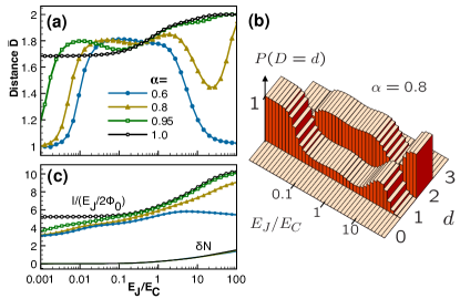
Figure 3: (Color online) (a) Average many-body distance $\bar{D}$ between the left- and right-going current states forming the ground state of a three-junction flux qubit at $f=0.5$, plotted as a function of $E_{J}/E_{C}$, for various asymmetry parameters $\alpha$. (b) Corresponding probability distribution for $\alpha=0.8$. (c) Magnitude $I$ of the average current in the two current states, and average charge fluctuation $\delta N$ in the ground state (symbols as in (a)).

Figure 3 shows the resulting average distance $\bar{D}$ (calculated with $\Delta n=6$). The fact that $D\geq 1$ is a consequence of defining the two states $\left|A\right\rangle$ and $\left|B\right\rangle$ as the eigenstates of the hermitean current operator, which makes them orthogonal by default, thus $P(D=0)=0$. At $\alpha=1$, the monotonic rise of $\bar{D}$ with $E_{J}/E_{C}$ is expected, as a larger $E_{J}/E_{C}$ allows the charges on each island to fluctuate more strongly, implying that more Cooper pairs can effectively contribute to the current states. The nonmonotonic dependence on $E_{J}/E_{C}$ for $\alpha<1$ was unexpected, but is likely due to the fact that smaller values of $\alpha$ tend to make the two counterpropagating current states no longer a “good” basis (the ring is broken for $\alpha=0$). In Fig. 3 (c), we have plotted both the expectation value of the current operator in one of the two superimposed states, as well as the average particle number fluctuation $\delta N$ in the ground state, where $\delta N^{2}\equiv\frac{1}{3}\sum_{j=1}^{3}\left\langle\left(\hat{n}_{j}-\left\langle\hat{n}_{j}\right\rangle\right)^{2}\right\rangle$. Evidently, neither of these quantities can be directly correlated to the average distance $\bar{D}$, apart from the general trend for all of them to usually increase with increasing $E_{J}/E_{C}$.

What is initially surprising is the fact that the distance remains small, although the examples discussed earlier clearly show that much larger distances may be reached in principle when applying our measure. In contrast, the “disconnectivity” for the Delft setup was estimated Leggett (2002) to be on the order of $10^{6}$, although a rigorous calculation seems very hard to do. Two reasons underly our finding for the flux qubit: First, it appears that the flux qubit considered here is really not that far from the Cooper pair box. In the Cooper pair boxNakamura et al. (1999), only a single Cooper pair tunnels between two superconducting islands, yielding $D=1$. In fact, allowing only for a small charge fluctuation (e.g. $\Delta n=4$) on each island of the flux qubit system is sufficient to reproduce the exact low-lying energy levels of this Hamiltonian to high accuracy for the parameter range considered here, since the charge fluctuations grow only slowly with $E_{J}/E_{C}$, as observed in Fig. 3 (c) ($\delta N\sim(E_{J}/E_{C})^{1/4}$ at large $E_{J}/E_{C}$). This means from the outset that very large values for $D$ may not be expected. Second, when analyzing the structure of the generated Hilbert spaces $\mathcal{H}_{d}$, it becomes clear that the dimensions of those spaces grow very fast with $d$, due to the large number of combinations of different single particle operators that are applied. For that reason, it turns out that the “target state” $\left|B\right\rangle=\left|-I\right\rangle$ can accurately be represented as a superposition of vectors lying within the first few of those spaces, yielding a rather small distance $\bar{D}$.

Outlook. - Our measure for the “size” of Schrödinger cat states can be applied, in principle, to any superposition of many-body states with constant particle number. Future challenges include the extension to states without a fixed particle number and the comparison to other measures, besides the DSC result Dür et al. (2002). In those cases where different particles couple to independent environments (as was assumed in DSC), our measure is expected to be an indication of the decoherence rate with which the corresponding superposition is destroyed, and it would be interesting to verify this in specific cases. Finally, we note that applications to many other physical systems are in principle straightforward, though the fast growth of Hilbert spaces may represent a significant hurdle for the direct numerical approach used here, and more efficient approximations would be desirable.

Acknowledgements. - We thank I. Cirac, who drew our attention to the question addressed here, as well as J. Clarke, K. Harmans, J. Korsbakken, A. J. Leggett, J. Majer, B. Whaley, F. Wilhelm and W. Zwerger for fruitful discussions. This work was supported by the SFB 631 of the DFG.

References

- Schrödinger (1935) E. Schrödinger, Naturwissenschaften 23, 807 (1935).
- Raimond et al. (2001) J. M. Raimond, M. Brune, and S. Haroche, Rev. Mod. Phys. 73, 565 (2001).
- Mooij et al. (1999) J. E. Mooij, T. P. Orlando, L. Levitov, L. Tian, C. H. van der Wal, and S. Lloyd, Science 285, 1036 (1999).
- van der Wal et al. (2000) C. H. van der Wal et al., Science 290, 773 (2000).
- Friedman et al. (2000) J. R. Friedman, V. Patel, W. Chen, S. K. Tolpygo, and J. E. Lukens, Nature 406, 43 (2000).
- Marquardt and Bruder (2001) F. Marquardt and C. Bruder, Phys. Rev. B 63, 054514 (2001).
- Buisson and Hekking (2001) O. Buisson and F. Hekking, in: Macroscopic Quantum Coherence and Quantum Computing (Kluwer, New York, 2001).
- Vion et al. (2002) D. Vion et al., Science 296, 886 (2002).
- Mancini et al. (1997) S. Mancini, V. I. Manko, and P. Tombesi, Phys. Rev. A 55, 3042 (1997).
- Marshall et al. (2003) W. Marshall, C. Simon, R. Penrose, and D. Bouwmeester, Physical Review Letters 91, 130401 (2003).
- Armour et al. (2002) A. D. Armour, M. P. Blencowe, and K. C. Schwab, Phys. Rev. Lett. 88, 148301 (2002).
- Arndt et al. (1999) M. Arndt et al., Nature 401, 680 (1999).
- Awschalom et al. (1992) D. D. Awschalom, J. F. Smyth, G. Grinstein, D. P. DiVincenzo, and D. Loss, Phys. Rev. Lett. 68, 3092 (1992).
- Julsgaard et al. (2001) B. Julsgaard, A. Kozhekin, and E. S. Polzik, Nature 413, 400 (2001).
- Leggett (2002) A. J. Leggett, J. Phys.: Condens. Matter 14, R415 (2002).
- Leggett (1980) A. J. Leggett, Prog. Theor. Phys. Suppl. 69, 80 (1980).
- Björk and Mana (2004) G. Björk and P. G. L. Mana, quant-ph/0310193 (2004).
- Dür et al. (2002) W. Dür, C. Simon, and J. I. Cirac, Phys. Rev. Lett. 89, 210402 (2002).
- Orlando et al. (1999) T. P. Orlando et al., Phys. Rev. B 60, 15398 (1999).
- Nakamura et al. (1999) Y. Nakamura, Y. A. Pashkin, and J. S. Tsai, Nature 398, 786 (1999).