On two-dimensional Bessel functions

Abstract

The general properties of two-dimensional generalized Bessel functions are discussed. Various asymptotic approximations are derived and applied to analyze the basic structure of the two-dimensional Bessel functions as well as their nodal lines.

1 Introduction

Generalized Bessel functions depending on several variables have been introduced in 1915 for a finite [1] and also an infinite number of variables [2]. They have very similar properties as the ordinary Bessel functions but are much less familiar. More recently, however, they found an increasing number of applications in various areas of physics (see, e.g., [3, 4, 5, 6, 7, 8, 9, 10, 11, 12, 13]). The basic theory of generalized Bessel functions is described in a mongraph by Dattoli and Torre [14]. Our own interest into the properties of these functions is caused by our recent studies of quantum dynamics in periodic structures [11, 12], in particular in studies of transport and dynamic localization [15].

In most cases these applications were restricted to the case of two variables, $u$ and $v$. Then the generalized Bessel functions  $J_{n}^{p,q}(u,v)$  are labeled by three integer indices $n,p,q$. The special case $(p,q)=(1,2)$ has been considered up to now almost exclusively [5, 10, 16, 17, 18, 8, 14]. Here we will analyze the two-dimensional Bessel functions  $J_{n}^{p,q}(u,v)$  for general indices $p$ and $q$ (see [19] for a well written introduction to the case of infinite variables).

We will derive the fundamental properties of the two-dimensional Bessel functions and analyze their basic structure for small and large arguments in the following sections. It will be seen that the two-dimensional Bessel functions show a rich oscillatory structure with regions of very different behavior. We will analyze these structural features with special attention to the nodal lines which are of considerable importance for recent applications to localization phenomena in quantum dynamics [15].

2 Basic properties

In this section we will collect the basic properties of the generalized Bessel functions  $J_{n}^{p,q}(u,v)$  with integer indices $n,\,p,\,q$ and two real arguments $u,\,v$. Most of the results in the literature (see, in particular, appendix B of [5] and chapter 2 of [14]) have been derived for the special case of  $J_{n}^{1,2}(u,v)$ .

2.1 Definition

The two-dimensional Bessel functions can be defined by the generating function

$${\rm e}^{{\rm i}(u\sin pt+v\sin qt)}=\sum\limits_{n=-\infty}^{\infty}J_{n}^{p,q}(u,v)\,{\rm e}^{{\rm i}nt}\,,$$ (1)

also known as a Jacobi-Anger expansion, or, somewhat more general, as

$$\exp\Big{(}\,\frac{u}{2}(z^{p}-z^{-p})+\frac{v}{2}(z^{q}-z^{-q})\,\Big{)}=\sum\limits_{n=-\infty}^{\infty}J_{n}^{p,q}(u,v)\,z^{n}\,.$$ (2)

Integration of (1) over $t$ using  $\int_{-\pi}^{+\pi}{\rm d}t\,{\rm e}^{{\rm i}nt}=2\pi\delta_{n,0}$ immediately leads to the integral representation

$$J_{n}^{p,q}(u,v)=\frac{1}{2\pi}\int_{-\pi}^{+\pi}{\rm d}t\,{\rm e}^{{\rm i}(u\sin pt+v\sin qt-nt)}\,,$$ (3)

a generalization of the integral representation of the well known ordinary Bessel function

$$J_{n}(x)=\frac{1}{2\pi}\int_{-\pi}^{+\pi}{\rm d}t\,{\rm e}^{{\rm i}(x\sin t-nt)}\,.$$ (4)

From the properties of Fourier series we immediately find the bounds

$$|J_{0}^{p,q}(u,v)|\leq 1\ \mbox{ and }\ |J_{n}^{p,q}(u,v)|\leq 1/\sqrt{2}\ \mbox{ for }\ n\neq 0\,.$$ (5)

As an immediate consequence of (3) the integers $p$ and $q$ can be assumed to be coprime because $J_{n}^{p,q}$ vanishes otherwise or it can be reduced to such a coprime case. This is seen as follows (we assume that $\mu$ is an integer, $0\neq\mu\neq 1$):

$$2\pi J_{n}^{\mu p,\mu q}(u,v)=\int_{0}^{2\pi}{\rm d}t\,{\rm e}^{{\rm i}(u\sin\mu pt+v\sin\mu qt-nt)}$$

$$=\int_{0}^{2\pi\mu}\frac{{\rm d}s}{\mu}\,{\rm e}^{{\rm i}(u\sin ps+v\sin qs-ns/\mu)}=\sum_{m=1}^{\mu}\int_{2\pi(m-1)}^{2\pi m}\frac{{\rm d}s}{\mu}\,{\rm e}^{{\rm i}(u\sin ps+v\sin qs-ns/\mu)}$$

$$=\Big{[}\sum_{m=1}^{\mu}{\rm e}^{-{\rm i}2\pi(m-1)n/\mu}\Big{]}\int_{0}^{2\pi}\frac{{\rm d}s}{\mu}\,{\rm e}^{{\rm i}(u\sin ps+v\sin qs-ns/\mu)}\,.$$ (6)

Using

$$\sum_{m=1}^{\mu}{\rm e}^{-{\rm i}2\pi(m-1)n/\mu}=\left\{\begin{array}[]{ll}\mu&\mbox{for }n/\mu\in\mathbb{Z}\\ 0&\mbox{else}\end{array}\right.$$ (9)

and – for $n/\mu\in\mathbb{Z}$ –

$$\int_{0}^{2\pi}\frac{{\rm d}s}{\mu}\,{\rm e}^{{\rm i}(u\sin ps+v\sin qs-ns/\mu)}=\frac{1}{\mu}\,J_{n/\mu}^{p,q}(u,v)$$ (10)

one obtains

$$J_{n}^{\mu p,\mu q}(u,v)=\left\{\begin{array}[]{ll}J_{n/\mu}^{p,q}(u,v)&\mbox{for }n/\mu\in\mathbb{Z}\\ 0&\mbox{else}\,.\end{array}\right.$$ (13)

In the following, we will therefore assume that the integers $p$ and $q$ have no common divisor.

2.2 Decomposition in terms of ordinary Bessel functions

A representation in terms of ordinary Bessel functions can be derived from the integral representation (3). Inserting the generating function for the ordinary Bessel functions

$${\rm e}^{{\rm i}x\sin s}=\sum\limits_{n=-\infty}^{\infty}J_{n}(x)\,{\rm e}^{{\rm i}ns}$$ (14)

for both $s=pt$ and $s=qt$ into (3), we obtain

$$J_{n}^{p,q}(u,v) = \frac{1}{2\pi}\int_{-\pi}^{+\pi}{\rm d}t\,{\rm e}^{{\rm i}(u\sin pt+v\sin qt-nt)}$$ (15)

$$= \sum_{\mu,\nu}J_{\mu}(u)\,J_{\nu}(v)\frac{1}{2\pi}\int_{-\pi}^{+\pi}{\rm d}t\,{\rm e}^{{\rm i}[(\mu p+\nu q-n)t]}\,.$$

The integral is only different from zero if  $n=\mu p+\nu q$  is satisfied. If $p$ and $q$ have no common divisor as assumed here, a solution $(\mu,\nu)=(M,N)$ of this Diophantine equation always exists and can be found systematically by, e.g., the Euclid algorithm [20]. Moreover there is an infinite number of solutions  $\mu=M-qk$, $\nu=N+pk$, $k=0,\pm 1,\pm 2,\,...$  because of

$$n=pM+qN=pM+qN+pqk-pqk=p(M-qk)+q(N+pk)\,.$$

We therefore have

$$J_{n}^{p,q}(u,v) = \sum\limits_{k=-\infty}^{\infty}J_{M-qk}(u)\,J_{N+pk}(v)\,,$$ (16)

where $(M,N)$ is an arbitrary solution of $n=pM+qN$.

For the case $p=1$ this reads ($M=n$ and $N=0$)

$$J_{n}^{1,q}(u,v)=\sum\limits_{k=-\infty}^{\infty}J_{n-qk}(u)\,J_{k}(v)\,.$$ (17)

In most of the previous applications one encounters the case $q=2$ and in these cases one usually simplifies the notation by dropping the $p,q$ indices, i.e. one defines

$$J_{n}(u,v)=J_{n}^{1,2}(u,v)\,.$$ (18)

2.3 Addition theorems

The addition theorem

$$J_{n}^{p,q}(u_{1}+u_{2},v_{1}+v_{2})=\sum\limits_{k=-\infty}^{\infty}J_{n-k}^{p,q}(u_{1},v_{1})\,J_{k}^{p,q}(u_{2},v_{2})$$ (19)

can be easily proved starting from (3) using (1):

$$J_{n}^{p,q}(u_{1}+u_{2},v_{1}+v_{2})=\frac{1}{2\pi}\int_{-\pi}^{+\pi}{\rm d}t\,{\rm e}^{{\rm i}(u_{1}\sin pt+v_{1}\sin qt-nt)}\,{\rm e}^{{\rm i}(u_{2}\sin pt+v_{2}\sin qt)}$$

$$=\frac{1}{2\pi}\int_{-\pi}^{+\pi}{\rm d}t\,{\rm e}^{{\rm i}(u_{1}\sin pt+v_{1}\sin qt-nt)}\sum\limits_{k=-\infty}^{\infty}J_{k}^{p,q}(u_{2},v_{2})\,{\rm e}^{{\rm i}kt}$$

$$=\sum\limits_{k=-\infty}^{\infty}J_{k}^{p,q}(u_{2},v_{2})\ \frac{1}{2\pi}\int_{-\pi}^{+\pi}{\rm d}t\,{\rm e}^{{\rm i}(u_{1}\sin pt+v_{1}\sin qt-(n-k)t)}$$

$$=\sum\limits_{k=-\infty}^{\infty}J_{k}^{p,q}(u_{2},v_{2})\,J_{n-k}^{p,q}(u_{1},v_{1})\,.$$

The Graf addition theorem for ordinary Bessel functions,

$$\sum_{\ell=-\infty}^{+\infty}\tau^{\ell}J_{\ell}(x_{1})J_{n+\ell}(x_{2})=\left[\frac{x_{2}-x_{1}/\tau}{x_{2}-x_{1}\tau}\right]^{\frac{n}{2}}J_{n}[g(x_{1},x_{2};\tau)]$$ (20)

with

$$\qquad g(x_{1},x_{2};\tau)=\big{(}x_{1}^{2}+x_{2}^{2}-x_{1}x_{2}(\tau+1/\tau)\big{)}^{1/2}\,,$$ (21)

can also be generalized to the two-dimensional case, at least for $p=1$ in the form

$$\sum_{\ell=-\infty}^{+\infty}\tau^{\ell}J_{\ell}^{1,q}(u_{1},v_{1})J_{n+\ell}^{1,q}(u_{2},v_{2})$$ (22)

$$=\sum_{\ell=-\infty}^{+\infty}\left[\frac{u_{2}-u_{1}/\tau}{u_{2}-u_{1}\tau}\right]^{\frac{n-q\ell}{2}}\left[\frac{v_{2}-v_{1}/\tau^{q}}{v_{2}-v_{1}\tau^{q}}\right]^{\frac{\ell}{2}}J_{n-q\ell}[g(u_{1},u_{2};\tau)]\,J_{\ell}[g(v_{1},v_{2};\tau^{q})]$$

(see Dattoli et al. [16, 14] for the special case $q=2$). The generalized Graf addition theorem (22) can be derived in a straightforward calculation expressing first the two-dimensional Bessel functions as a sum over ordinary ones (see eqn. (17)) and using the Graf addition theorem (20) for ordinary Bessel functions:

$$\sum_{\ell=-\infty}^{+\infty}\tau^{\ell}J_{\ell}^{1,q}(u_{1},v_{1})J_{n+\ell}^{1,q}(u_{2},v_{2})$$ (23)

$$\ =\sum_{\ell,j,k}\tau^{\ell}J_{\ell-qk}(u_{1})J_{k}(v_{1})J_{\ell+n-qj}(u_{2})J_{j}(v_{2})$$

$$\ =\sum_{j,k}J_{k}(v_{1})J_{j}(v_{2})\,\tau^{qk}\sum_{\ell^{\prime}}\tau^{\ell^{\prime}}J_{\ell^{\prime}}(u_{1})J_{n+q(k-j)+\ell^{\prime}}(u_{2})$$

$$\ =\sum_{j,k}J_{k}(v_{1})J_{j}(v_{2})\,\tau^{qk}J_{n+q(k-j)}(g(u_{1},u_{2};\tau))\left[\frac{u_{2}-u_{1}/\tau}{u_{2}-u_{1}\tau}\right]^{\frac{n+q(k-j)}{2}}$$

$$\ =\sum_{\ell}\left[\frac{u_{2}-u_{1}/\tau}{u_{2}-u_{1}\tau}\right]^{\frac{n-q\ell}{2}}\!\!J_{n-q\ell}(g(u_{1},u_{2};\tau))\sum_{k}\tau^{qk}J_{k}(v_{1})J_{\ell+k}(v_{2})$$

$$\ =\sum_{\ell}\left[\frac{u_{2}-u_{1}/\tau}{u_{2}-u_{1}\tau}\right]^{\frac{n-q\ell}{2}}\!\!\left[\frac{v_{2}-v_{1}/\tau^{q}}{v_{2}-v_{1}\tau^{q}}\right]^{\frac{\ell}{2}}\!\!J_{n-q\ell}(g(u_{1},u_{2};\tau))J_{\ell}(g(v_{1},v_{2};\tau^{q}))$$

with  $g(x_{1},x_{2};\tau)$  as defined in (21).

2.4 Symmetries, special cases and numerical examples

From the definition (1) one verifies (by taking the complex conjugate and changing variables $t\rightarrow-t$) that the  $J_{n}^{p,q}(u,v)$  are real valued and satisfy

$$J_{n}^{p,q}(0,0)=\delta_{n0}\,.$$ (24)

The symmetry relations

$$J_{n}^{p,q}(u,v) = J_{n}^{q,p}(v,u)$$ (25)

$$J_{-n}^{p,q}(u,v) = J_{n}^{p,q}(-u,-v)=J_{n}^{q,p}(-v,-u)=J_{n}^{-p,-q}(u,v)\,.$$ (26)

follow directly from the definition. For $n=0$ these equations imply the symmetries

$$J_{0}^{p,q}(u,v)=J_{0}^{p,q}(-u,-v)=J_{0}^{q,p}(v,u)\,.$$ (27)

A further direct result is a symmetry relation for even values of one of the $p,q$-indices, say $q$. Using $J_{n}(-z)=(-1)^{n}\,J_{n}(z)$ we get

$$J_{n}^{p,q}(-u,v)=\sum\limits_{k=-\infty}^{\infty}J_{M-qk}(-u)\,J_{N+pk}(v)$$

$$\quad=(-1)^{M}\sum\limits_{k=-\infty}^{\infty}J_{M-qk}(u)\,J_{N+pk}(v)=(-1)^{n}\,J_{n}^{p,q}(u,v)\,.$$ (28)

The last equality holds because of $(-1)^{n}=(-1)^{pM+qN}=(-1)^{M}$ for $q$ even and $p$ odd. This symmetry implies

$$J_{n}^{p,q}(0,v)=(-1)^{n}J_{n}^{p,q}(0,v)\ \Longrightarrow\ J_{n}^{p,q}(0,v)=0\mbox{ for }n\mbox{ odd and }q\mbox{ even}.$$ (29)

If both upper indices are odd, their difference must be even. This leads to another symmetry relation

$$J_{n}^{p,q}(-u,-v)=\sum\limits_{k=-\infty}^{\infty}J_{M-qk}(-u)\,J_{N+pk}(-v)$$

$$\qquad=\sum\limits_{k=-\infty}^{\infty}(-1)^{M+N+(p-q)k}J_{M-qk}(u)\,J_{N+pk}(v)$$ (30)

$$\qquad=(-1)^{M+N}\,J_{n}^{p,q}(u,v)=(-1)^{n}\,J_{n}^{p,q}(u,v)\quad\mbox{for }p,q\mbox{ odd}\,.$$

Here the last equality is based on the fact that for odd $p,q$-indices, $p=2j+1$ and $q=2k+1$, we have $n=pM+qN=M+N+2(j+k)$.

In the case $p=q$ the two-dimensional Bessel functions simplify and reduce to ordinary Bessel functions if $n$ is an integer multiple of $p$:

$$J_{n}^{p,p}(u,v) = \frac{1}{2\pi}\int_{-\pi}^{+\pi}{\rm d}t\,{\rm e}^{{\rm i}((u+v)\sin pt-nt)}=\frac{1}{2\pi}\int_{-p\pi}^{+p\pi}\frac{{\rm d}s}{p}\,{\rm e}^{{\rm i}((u+v)\sin s-ns/p)}$$ (33)

$$= \left\{\begin{array}[]{ll}J_{n/p}(u+v)&\mbox{for }n/p\in\mathbb{N}\\ 0&\mbox{else}\,.\end{array}\right.$$

Another relation between the generalized and ordinary Bessel functions can be observed if the index $n$ is a multiple of one of the upper indices, e.g. $n=mq$, $m$ integer. Then we get

$$J_{mq}^{p,q}(0,v) = \frac{1}{2\pi}\int_{-\pi}^{+\pi}{\rm d}t\,{\rm e}^{{\rm i}(v\sin qt-mqt)}=\frac{1}{2\pi q}\int_{-q\pi}^{q\pi}{\rm d}s\,{\rm e}^{{\rm i}(v\sin s-ms)}$$ (34)

$$= \frac{1}{2\pi}\int_{-\pi}^{+\pi}{\rm d}s\,{\rm e}^{{\rm i}(v\sin s-ms)}=J_{m}(v)$$

and, as a special case,

$$J_{n}^{p,1}(0,v)=J_{n}(v)\,.$$ (35)

According to (34) the two-dimensional Bessel function $J_{n}^{p,q}(0,v)$ is reduced to an ordinary Bessel function $J_{m}(v)$ for $n=mq$. Otherwise the function vanishes on the $v$-axis as can easily be seen from (16):

$$J_{n}^{p,q}(0,v)\!=\!\sum\limits_{k=-\infty}^{\infty}J_{M-qk}(0)\,J_{N+pk}(v)\!=\!\sum\limits_{k=-\infty}^{\infty}\delta_{M,qk}\,J_{N+pk}(v)=0\,,$$ (36)

if $M$ is not a multiple of $q$ or, equivalently,  $n=pM+qN$  is not an integer multiple of $q$. We therefore have

$$J_{n}^{p,q}(0,v)=0\quad\mbox{if}\ n\neq mq,\ m\in\mathbb{Z}$$ (37)

as a generalization of (29).

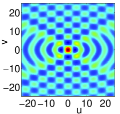
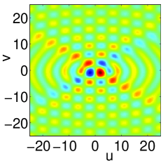
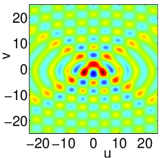
Figure 1: Color map of the two-dimensional Bessel function $J_{n}^{1,2}(u,v)$ for $n=0$, $n=1$, $n=2$ (from left to right).

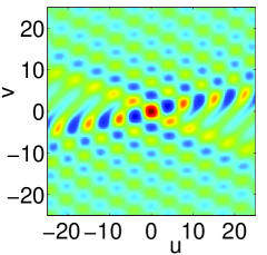
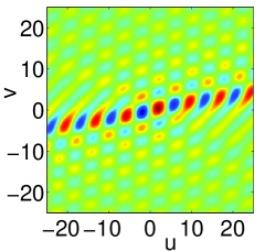
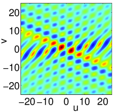
Figure 2: Color map of the two-dimensional Bessel function $J_{n}^{1,3}(u,v)$ for $n=0$, $n=1$, $n=2$ (from left to right).

Let us look at a few examples of two-dimensional Bessel functions calculated numerically using the representation (16) in terms of ordinary Bessel functions (similar graphs can be found, e.g., in [17, 14]). Figures 1 and 2 show color maps of $J_{n}^{1,2}(u,v)$ and $J_{n}^{1,3}(u,v)$ for $n=0$, $n=1$ and $n=2$ using a re-normalization to unit maximum in each case (the regions of positive values are colored red, of negative ones blue).

For $J_{n}^{1,2}$ in figure 1 we see that the symmetry relations

$$J_{0}^{1,2}(-u,-v)=J_{0}^{1,2}(u,v)\quad,\quad J_{n}^{1,2}(-u,v)=(-1)^{n}\,J_{n}^{1,2}(u,v)$$ (38)

are satisfied (compare eqs. (27) and (28) ). The last relation implies a nodal line for $n=1$ along the $v$-axis,  $J_{1}^{1,2}(0,v)=0$. For the case $J_{n}^{1,3}(-u,-v)$ in figure 2 we have the symmetry  $J_{n}^{1,3}(-u,-v)=(-1)^{n}\,J_{n}^{1,3}(u,v)$  (compare eq. (2.4)).

2.5 Sum rules and Kapteyn series

The simple sum rule

$$\sum\limits_{n=-\infty}^{\infty}J_{n}^{p,q}(u,v)=1$$ (39)

is a direct consequence of the generating function (1) for $t=0$. A variety of sum rules for special cases can be obtained by choosing $t$ in (1) appropriately. E.g. for the important special case $(p,q)=(1,2)$ another sum rule is found by setting $t=\pi/2$:

$$\sum\limits_{n=-\infty}^{\infty}{\rm i}^{n}\,J_{n}^{1,2}(u,v)={\rm e}^{{\rm i}u}\,.$$ (40)

Similar sum rules can be obtained for other special cases. Another sum rule,

$$\sum\limits_{k=-\infty}^{\infty}\big{(}J_{k}^{p,q}(u,v)\big{)}^{2}=1$$ (41)

follows from the addition theorem (19) for the special case $n=0$, $u_{1}=-u_{2}=u$, $v_{1}=-v_{2}=v$ using (24).

We furthermore note without proof the Kapteyn type series [21, 22]

$$\sum\limits_{n=-\infty}^{\infty}J_{n}^{p,q}(nu,nv)=\frac{1}{1-pu-qv}\quad,\quad|pu|+|qv|<1\,.$$ (42)

2.6 Further generalizations

As already stated in the introduction, the number of variables in the Bessel function can be extended. Different types of generalizations are, however, also possible. Modified higher dimensional Bessel functions can be constructed, e.g. by replacing one of the ordinary Bessel functions in (16) by a modified one [9]. In addition, two-variable, one-parameter Bessel functions [9, 23] can be defined as a generalization of (16):

$$J_{n}^{p,q}(u,v;\tau) = \sum\limits_{k=-\infty}^{\infty}J_{M-qk}(u)\,J_{N+pk}(v)\,\tau^{k}$$ (43)

(Let us recall that $(M,N)$ are arbitrary solutions of $n=pM+qN$.) Here again we find  $J_{n}^{p,q}(0,0;\tau)=\delta_{n0}$ .

In particular the case $\tau={\rm e}^{{\rm i}\delta}$ is of interest [9, 15] for applications in physics. We confine ourselves to the most important case $p=1$, i.e.

$$J_{n}^{1,q}(u,v;{\rm e}^{{\rm i}\delta}) = \sum\limits_{k=-\infty}^{\infty}J_{n-qk}(u)\,J_{k}(v){\rm e}^{{\rm i}k\delta}\,.$$ (44)

Following the lines in the derivations above, one can easily show that these functions are generated by

$${\rm e}^{{\rm i}(u\sin t+v\sin(qt+\delta))}=\sum\limits_{n=-\infty}^{\infty}J_{n}^{1,q}(u,v;{\rm e}^{{\rm i}\delta})\,{\rm e}^{{\rm i}nt}\,,$$ (45)

which leads to the integral representation

$$J_{n}^{1,q}(u,v;{\rm e}^{{\rm i}\delta})=\frac{1}{2\pi}\int_{-\pi}^{+\pi}{\rm d}t\,{\rm e}^{{\rm i}(u\sin t+v\sin(qt+\delta)-nt)}\,.$$ (46)

The generalized Bessel functions  $J_{n}^{1,q}(u,v;{\rm e}^{{\rm i}\delta})$  satisfy most of the properties of the  $J_{n}^{1,q}(u,v)$ , as for example the bounds (5), the addition theorem (19) and the sum rules (39) and (41). These function are, however, complex valued.

Figure 3 shows the real part of the Bessel functions $J_{n}^{1,2}(u,v;{\rm i})$ for $n=0,\,1,\,2$. A comparison with figure 1 shows that the structure of the functions is strongly altered by the angle parameter $\delta$.

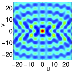
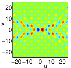
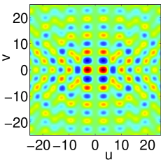
Figure 3: Color map of the two-dimensional, one-parameter Bessel function $J_{n}^{1,2}(u,v;{\rm i})$ for $n=0$, $n=1$, $n=2$ (from left to right). The figures show the real part.

2.7 Differential equations and recurrence relations

Finally, we will derive recurrence relations for the $J_{n}^{p,q}(u,v)$ and their derivatives. Differentiating the generating function (2) with respect to $u$ leads to

$${\textstyle\frac{1}{2}}\big{(}z^{p}-z^{-p}\big{)}\,{\rm e}^{\textstyle\frac{u}{2}(z^{p}-z^{-p})+\frac{v}{2}(z^{q}-z^{-q})}$$

$$\quad={\textstyle\frac{1}{2}}\sum\limits_{n=-\infty}^{\infty}J_{n}^{p,q}(u,v)\,\big{(}z^{n+p}-z^{n-p}\big{)}=\sum\limits_{n=-\infty}^{\infty}\partial_{u}J_{n}^{p,q}(u,v)\,z^{n}\,.$$ (47)

Equating the coefficients of $z^{n}$, we find

$$2\,\partial_{u}J_{n}^{p,q}(u,v)=J_{n-p}^{p,q}(u,v)-J_{n+p}^{p,q}(u,v)$$ (48)

and similarly

$$2\partial_{v}J_{n}^{p,q}(u,v)=J_{n-q}^{p,q}(u,v)-J_{n+q}^{p,q}(u,v)\,.$$ (49)

If we differentiate (2) with respect to $z$ and compare the coefficients, we find the recurrence equation

$$pu\,\big{(}J_{n-p}^{p,q}(u,v)\!+\!J_{n+p}^{p,q}(u,v)\big{)}\!+\!qv\,\big{(}J_{n-q}^{p,q}(u,v)\!+\!J_{n+q}^{p,q}(u,v)\big{)}\!=\!2nJ_{n}^{p,q}(u,v)\,.$$ (50)

These are generalizations of the relations derived by Reiss [5] for the case $J_{n}^{1,2}(u,v)$.

Similarly one can show that the derivatives of the generalized Bessel functions (44) are given by

$$2\partial_{u}J^{1,q}_{n}(u,v;{\rm e}^{{\rm i}\delta})=J^{1,q}_{n-1}(u,v;{\rm e}^{{\rm i}\delta})-J^{1,q}_{n+1}(u,v;{\rm e}^{{\rm i}\delta})$$

$$2\partial_{v}J^{1,q}_{n}(u,v;{\rm e}^{{\rm i}\delta})={\rm e}^{{\rm i}\delta}J^{1,q}_{n-q}(u,v;{\rm e}^{{\rm i}\delta})-{\rm e}^{-{\rm i}\delta}J^{1,q}_{n+q}(u,v;{\rm e}^{{\rm i}\delta}).$$ (51)

Using these relations one can show that the two-dimensional Bessel functions solve a variety of linear partial differential equations, depending on their indices $(p,q)$. These differential equation can be constructed systematically by adding up derivatives of different order such that the different terms $~{}J^{p,q}_{n}$ cancel each other for every value of $n$. For example the ordinary two-dimensional Bessel functions with $q=p$ solve the wave equation

$$\left(\partial_{u}^{2}-\partial_{v}^{2}\right)J_{n}^{1,1}(u,v)=0,$$ (52)

while the generalized Bessel functions with $(p,q)=(1,2)$ and $\delta=\pi/2$ solve the time-dependent Schrödinger equation [17, 24]

$${\rm i}\partial_{v}J^{1,2}_{n}(u,v;{\rm i})=\left(-2\partial_{u}^{2}-1\right)J^{1,2}_{n}(u,v;{\rm i}).$$ (53)

Furthermore, a repeated application of the differentiation rules (48), (49) and the recurrence relations (50) leads to the coupled differential equations

$$\left[\left(pu\partial_{u}+qv\partial_{v}\right)^{2}+\left(p^{2}u\partial_{u}+q^{2}v\partial_{v}\right)+p^{2}u^{2}+q^{2}v^{2}-n^{2}\right]J^{p,q}_{n}(u,v)$$

$$\quad=-pquv\left(J^{p,q}_{n-p+q}(u,v)+J^{p,q}_{n+p-q}(u,v)-2J^{p,q}_{n}(u,v)\right)$$ (54)

for arbitrary indices $(p,q)$. Except from the right-hand side this equation is structurally similar to the defining differential equation of the ordinary one-dimensional Bessel functions. Equations (54) can be decoupled for $q=\nu p,\;\nu\in\mathbb{Z}$ by applying again (50). For $(p,q)=(1,\pm 1)$ this yields

$$\left[\left(u\partial_{u}+v\partial_{v}\right)^{2}+\left(u\partial_{u}+v\partial_{v}\right)+(u\pm v)^{2}-n^{2}\right]J^{1,\pm 1}_{n}(u,v)=0,$$ (55)

while the respective calculations for other values of $q$ lead to more complicated results.

3 Polynomial expansion for small arguments

We will first analyze the regime of small arguments $u$ and $v$ and derive a leading order polynomial expansion. Following Wasiljeff [4], we expand the $u,v$-dependent part of the exponential function in (3) in a Taylor series:

$$J^{p,q}_{n}(u,v)=\frac{1}{2\pi}\int\limits_{-\pi}^{+\pi}{\rm e}^{{\rm i}(u\sin{pt}+v\sin{qt}-nt)}{\rm d}t$$ (56)

$$\quad=\frac{1}{2\pi}\sum\limits_{k=0}^{\infty}\frac{1}{2^{k}k!}\int\limits_{-\pi}^{\pi}\big{(}u{\rm e}^{{\rm i}pt}-u{\rm e}^{-{\rm i}pt}+v{\rm e}^{{\rm i}qt}-v{\rm e}^{-{\rm i}qt}\big{)}^{k}\,{\rm e}^{-{\rm i}nt}{\rm d}t\,.$$ (57)

Using the polynomial formula

$$(a+b+c+d)^{j}=j!\sum\limits_{\alpha,\beta,\sigma,\zeta}\nolimits^{\,{}^{\prime}}\,\frac{a^{\alpha}\,}{\alpha!}\frac{b^{\beta}}{\beta!}\frac{c^{\sigma}}{\sigma!}\frac{d^{\zeta}}{\zeta!}\,,$$ (58)

where the primed sum runs over all indices with $j=\alpha+\beta+\sigma+\zeta$, one obtains after rearranging terms and carrying out the integration the series expansion

$$J^{p,q}_{n}(u,v)=\sum\limits_{j=0}^{\infty}\frac{1}{2^{j}}\sum\limits_{\alpha,\beta,\sigma,\zeta}\nolimits^{\,{}^{\prime\prime}}\frac{u^{\alpha+\beta}\,v^{\sigma+\zeta}}{\alpha!\,\beta!\,\sigma!\,\zeta!}\,.$$ (59)

Here the double-primed sum includes all nonnegative integers with

$$j=\alpha+\beta+\sigma+\zeta\quad\mbox{and}\quad n=(\alpha-\beta)p+(\sigma-\zeta)q\,.$$ (60)

The sum can be transformed into a more convenient form by introducing $\ell=\alpha+\beta$, $2f=\ell+\alpha-\beta$, $m=\sigma+\zeta$ and $2g=m+\sigma-\zeta$. After some elementary algebra, this yields

$$J^{p,q}_{n}(u,v)=\sum\limits_{\ell,m\geq 0}\,a_{\ell,m}^{(n,p,q)}\,\frac{u^{m}v^{\ell}}{2^{\ell+m}}$$ (61)

with

$$a_{\ell,m}^{(n,p,q)}=\sum_{\begin{subarray}{c}f=0,\ldots,+\ell\cr g=0,\ldots,+m\cr n=p(2f-\ell)+q(2g-m)\end{subarray}}\frac{1}{f!(\ell-f)!g!(m-g)!}\,.$$ (62)

The lowest order approximation in this expansion can be found in explicit form for the case $p=1$. Then the lowest order term in (59) is given by

$$\qquad(\alpha,\,\beta,\,\sigma,\,\zeta)=\left\{\begin{array}[]{ll}(n-q\lfloor\frac{n}{q}\rfloor,\,0,\,\lfloor\frac{n}{q}\rfloor,\,0)&\mbox{if }\frac{n}{q}\notin\mathbb{N}\mbox{ and }2q\,{\rm mod}(n,q)\leq q+1\\[5.69054pt] (0,\,-n+q\lceil\frac{n}{q}\rceil,\,\lceil\frac{n}{q}\rceil,0)&\mbox{if }\frac{n}{q}\notin\mathbb{N}\mbox{ and }2q\,{\rm mod}(n,q)\geq q+1\\[5.69054pt] (0,\,0,\,\frac{n}{q},\,0)&\mbox{if }\frac{n}{q}\in\mathbb{N}\,.\hfill(66)\end{array}\right.$$ (67)

In most cases it is given by a single term, as for example in

$$J_{3}^{1,2}(u,v)\sim\frac{1}{2^{2}}\,uv\quad,\quad J_{4}^{1,2}(u,v)\sim\frac{1}{2^{2}}\,v^{2}\,.$$ (68)

Note that, because $n=3$ is not a multiple of $q=2$, the Bessel function $J_{3}^{1,2}$ is identically equal to zero on the $v$-axis (see eq. (37)), however $J_{3}^{1,2}$ and $J_{4}^{1,2}$ do not vanish on the $u$-axis, where we have $J_{n}^{1,2}(u,0)=J_{n}(u)\sim(u/2)^{n}/n!$ (see eq. (35)).

In certain cases more terms of the same minimum order $j$ appear. This happens if $\frac{n}{q}\notin\mathbb{N}$ and $2q\,{\rm mod}(n,q)=q+1$. One can easily check that this requires that $q$ is odd, $q=2\nu+1$, and $n=\mu q+\nu+1$ with $\nu,\mu\in\mathbb{N}$. In this case, the lowest order approximation reads

$$J^{1,q}_{n}(u,v)\sim\frac{u^{\nu}v^{\mu}}{2^{\nu+\mu+1}\nu!\mu!}\left(\frac{u}{\nu+1}+\frac{v}{\mu+1}\right)\,.$$ (69)

This yields the (approximate) nodal line

$$v=-\frac{\mu+1}{\nu+1}\,u$$ (70)

for small $u$ and $v$. As an example, we note $q=5$ and $n=23$, i.e. $\nu=2$ and $\mu=4$ and therefore

$$J^{1,5}_{23}(u,v)\sim\frac{u^{2}v^{4}}{2^{7}2!4!}\left(\frac{u}{3}+\frac{v}{5}\right)\,.$$ (71)

4 Asymptotic approximations

In the examples of two-dimensional Bessel functions $J_{n}^{p,q}(u,v)$ shown in figures 1 and 2 for $(p,q)=(1,2)$ and $(p,q)=(1,3)$, respectively, one observes a rich oscillatory structure which will be analyzed in the following. The skeleton of this structure and valuable approximations can be obtained asymptotically by means of the stationary phase approximation

$$\int\limits_{-\pi}^{\pi}{\rm d}t\,h(t)\,{\rm e}^{{\rm i}\,g(t)}\simeq\sum_{t_{s}}{\textstyle\sqrt{\frac{2\pi}{\pm g^{\prime\prime}(t_{s})}\,}}\,h(t_{s})\,{\rm e}^{{\rm i}g(t_{s})\pm{\rm i}\pi/4}\,.$$ (72)

The sum extends over all contributing real stationary points and the $\pm$ sign is chosen so that $\pm g^{\prime\prime}(t_{s})$ is positive (see, e.g., [25] for more details). Previous studies of asymptotic approximations for two-dimensional Bessel functions [3, 26, 10] have been restricted to the case $p=1$, $q=2$ and special regions of the index $n$ and arguments $u,v$.

Information about the oscillatory structure of the multivariable Bessel functions $J_{n}^{p,q}(u,v)$ can be obtained from asymptotic approximations for large arguments and/or large indices. We will consider three of the large number of possible limits: the case when both arguments $u$ and $v$ are large, whereas $n$ remains fixed, and the case where one argument, $v$, and the index $n$ are large for fixed value of the argument $u$. Finally we will consider the limit where both variables as well as the index $n$ are large. In all cases we assume small fixed values of the indices $p$ and $q$.

4.1 Basic structure for large arguments $u$ and $v$

We base our analysis on the integral representation (3)

$$J_{n}^{p,q}(u,v)=\frac{1}{2\pi}\int_{-\pi}^{+\pi}{\rm d}t\,{\rm e}^{{\rm i}(\phi(t)-nt)}\ ,\quad\phi(t)=u\sin pt+v\sin qt\,.$$ (73)

Here we will consider the asymptotic limit of large arguments $u$ and $v$ assuming that $n$ is fixed, i.e. we identify $g(t)=\phi(t)$ in an application of (72). The condition

$$\phi^{\prime}(t)=pu\cos pt+qv\cos qt=0$$ (74)

determines the stationary points $t_{s}$ (note that there are always pairs of such stationary points with different sign due to the symmetry of the cosine-function). The integral (73) is then approximately given by

$$J_{n}^{p,q}(u,v)=\sum_{t_{s}}\frac{1}{\sqrt{2\pi|\phi^{\prime\prime}(t_{s})|}}\,{\rm e}^{{\rm i}(\phi(t_{j})-nt_{s}\pm\pi/4)}\,,$$ (75)

where the $\pm$-sign is given by the sign of $\phi^{\prime\prime}(t_{j})$. The main contribution to the sum is provided by real-valued stationary points, complex points lead to exponentially decaying terms. At the points where two stationary points coalesce when the arguments $u$ and $v$ are varied, the second derivative

$$\phi^{\prime\prime}(t)=-p^{2}u\sin pt-q^{2}v\sin qt$$ (76)

vanishes and the approximation diverges. Crossing these bifurcation points, the function changes its character. In the present case, the bifurcations are determined by the simultaneous solution of

$$pu\cos pt_{s}=-qv\cos qt_{s}\quad\mbox{and}\quad p^{2}u\sin pt_{s}=-q^{2}v\sin qt_{s}\,.$$ (77)

This can be most easily satisfied if both sides of one of the two equations are equal to zero. We distinguish two cases:
Case (i) $\sin pt_{s}=-\sin qt_{s}=0$ : For coprime $p$ and $q$, this implies $t_{s}=0$ or $t_{s}=\pi$ and therefore (from $pu\cos pt_{s}=-qv\cos qt_{s}$) we have $pu=-qv$ or $pu=-(-1)^{p+q}\,qv$, respectively. We therefore obtain the bifurcation lines

$$v=\pm p\,u/q\quad \mbox{if one of the }p,q\mbox{ is even}$$ (78)

$$v=-p\,u/q\quad \mbox{else }.$$ (79)

Case (ii) $\cos pt_{s}=\cos qt_{s}=0$ : This implies $pt_{s}=\pi/2+j\pi$ and $qt_{s}=\pi/2+k\pi$ with integer $j$ and $k$ or  $(2k+1)p=(2j+1)q$  and (for coprime $p$ and $q$)  $p=2j+1$  and  $q=2k+1$ . With  $\sin pt_{s}=\sin(\pi/2+j\pi)=(-1)^{j}$  and  $\sin qt_{s}=\sin(\pi/2+k\pi)=(-1)^{k}$  the second condition in (77) leads to

$$v=-(-1)^{j+k}\,u\,p^{2}/q^{2}\quad p=2j+1\ ,\ q=2k+1\,.$$ (80)

The examples in figure 1 show Bessel functions $J_{n}^{1,2}(u,v)$ for various values of $n$. Here $q$ is even and from equation (79) we find the bifurcation lines

$$v=\pm u/2\,.$$ (81)

We observe that the structure of the Bessel functions changes if one crosses these lines. In the left and right sectors, we have only two stationary points, $\pm t_{1}$, whereas in the upper and lower sectors we have four stationary points, $\pm t_{1}$ and $\pm t_{2}$, and consequently a richer interference pattern. This will be analyzed in more detail below.

For the two-dimensional Bessel function $J_{n}^{1,3}(u,v)$ displayed in fig. 2 both upper indices are odd and the bifurcation lines are given by eqs. (79) and (80):

$$v=-\,u/3\quad\mbox{and}\quad v=u/9\,.$$ (82)

The qualitative difference to the behavior of $J_{n}^{1,2}(u,v)$ in fig. 1 is obvious.

Let us now analyze the function  $J_{n}^{1,2}(u,v)$  in more detail working out explicitly the stationary phase approximation. In view of the symmetry $J_{n}^{1,2}(u,v)=J_{-n}^{1,2}(-u,-v)$ (26) we can assume $v>0$ in the following for simplicity. The stationary phase condition

$$u\cos t=-2v\,\cos 2t=-2v\,(2\cos^{2}t-1)$$ (83)

can be solved for $c=\cos t$ with solution

$$c_{\pm}=\frac{1}{8}\,\big{(}-u/v\pm\sqrt{(u/v)^{2}+32\,}\,\big{)}\,.$$ (84)

In the region $-2<u/v<+\infty$ the necessary condition $|c_{\pm}|\leq 1$ is met by $c_{+}$ and vice versa by $c_{-}$ in the region $-\infty<u/v<+2$. Note that in the interval $-2<u/v<+2$ both solutions fulfill $|c_{\pm}|\leq 1$. With  $t_{\pm}=\arccos c_{\pm}$  and  $\sin t_{\pm}=\pm\sqrt{1-c^{2}_{\pm}}$  we arrive at

$$\phi_{\pm} = u\sin t_{\pm}+v\sin 2t_{\pm}=\pm(u+2vc_{\pm})\,\sqrt{1-c^{2}_{\pm}}$$ (85)

$$\phi^{\prime\prime}_{\pm} = -u\sin t_{\pm}-4v\sin 2t_{\pm}=\mp(u+8vc_{\pm})\,\sqrt{1-c^{2}_{\pm}}$$ (86)

and with the definitions

$$F_{+}(u,v)\!\! = \!\!\left\{\begin{array}[]{l l}\sqrt{\frac{2}{\pi|\phi^{\prime\prime}_{+}|}}\,\cos\big{(}\phi_{+}-n\arccos c_{+}-\frac{\pi}{4}\big{)}&\mbox{for }-2v<u\\[5.69054pt] 0&\mbox{else }\end{array}\right.$$ (89)

$$F_{-}(u,v)\!\! = \!\!\left\{\begin{array}[]{l l}\sqrt{\frac{2}{\pi|\phi^{\prime\prime}_{-}|}}\,\cos\big{(}\phi_{-}+n\arccos c_{-}-\frac{\pi}{4}\big{)}&\mbox{for }u<+2v\\[5.69054pt] 0&\mbox{else }\end{array}\right.\,$$ (92)

the final result can be written as

$$J_{n}^{1,2}(u,v)\simeq F_{+}(u,v)+F_{-}(u,v)\,.$$ (93)

Here one should be aware of the fact that in the region  $|u|\ll 2|v|$  both of the terms $F_{\pm}(u,v)$ provide a non-vanishing contribution.

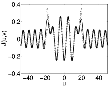
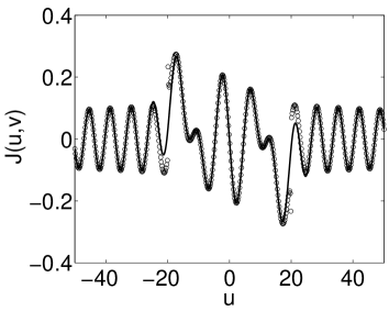
Figure 4: Two-dimensional Bessel functions $J_{n}^{1,2}(u,v)$ with $v=10$ for $n=0$ (left) and $n=1$ (right) as a function of $u$ (full curve) in comparison with the stationary phase approximation (93) (open circles).

This so-called ’primitive’ stationary phase approximation diverges at the bifurcation lines $v=\pm 2u$. If desired, it can be improved by taking complex stationary points into account and by taming the divergences by uniformization methods.

In the limit $|u|\rightarrow\infty$ the asymptotic approximation (93) simplifies drastically. Only $F_{+}$ contributes for $u>0$ ($F_{-}$ for $u<0$) and with $t_{\pm}=\pm\pi/2$, $\phi_{\pm}=\phi^{\prime\prime}_{\pm}=\pm u$ we find

$$J_{n}^{1,2}(u,v)\simeq\sqrt{\frac{2}{\pi|u|}}\,\cos\big{(}u-n\frac{\pi}{2}-\frac{\pi}{4}\big{)}\,,$$ (94)

which agrees with the well-known asymptotic approximation of the ordinary Bessel function $J_{n}(u)$ for large arguments [27]. In the alternative limit $v\rightarrow\infty$ both terms, $F_{+}$ and $F_{-}$ contribute. With $c_{\pm}=-\frac{u}{8v}\pm\frac{1}{\sqrt{2}}$, $\phi_{\pm}=v\pm\frac{u}{\sqrt{2}}$ and $\phi^{\prime\prime}_{\pm}=\pm 4v$ we obtain

$$J_{n}^{1,2}(u,v)\simeq\sqrt{\frac{2}{\pi v}}\left\{\begin{array}[]{ll}+\cos\big{(}v-(n+1)\frac{\pi}{4}\big{)}\,\cos\frac{u}{\sqrt{2}}&n\mbox{ even}\\[5.69054pt] -\sin\big{(}v-(n+1)\frac{\pi}{4}\big{)}\,\sin\frac{u}{\sqrt{2}}&n\mbox{ odd}\,,\end{array}\right.$$ (97)

as already derived in [14].

As an illustration of the asymptotic formula (93), fig. 4 shows the two-dimensional Bessel function $J_{n}^{1,2}(u,v)$ in comparison with the stationary phase approximation for $v=10$ and $n=0$, $1$. With the exception of the vicinity of the divergences at $u=\pm 2v=\pm 20$, the agreement is excellent. This approximation can be used in oder to determine the nodal lines of the two-dimensional Bessel functions which is of interest for applications in physics [15].

4.2 Large argument $v$ and large index $n$

In this section we will consider the regime where the index $n$ and one of the arguments, e.g. $v$, are large. In view of (26), we can assume $n\geq 0$. Following the analysis applied to the special case $J^{1,2}_{n}(u,v)$ by Reiss and Krainov [10], we separate the integral representation (3) into a fast, ${\rm e}^{{\rm i}g(t)}$, and a slowly oscillating part:

$$J^{p,q}_{n}(u,v)=\frac{1}{2\pi}\int\limits_{-\pi}^{\pi}{\rm d}t\,{\rm e}^{{\rm i}u\sin{pt}}{\rm e}^{{\rm i}g(t)}\quad,\quad g(t)=v\sin{qt}-nt\,,$$ (98)

and evaluate the integral approximately by the method of stationary phase or the saddle point method if the stationary points are complex valued (for details see, e.g., [25]).

The stationary points $t_{s}$ of $g(t)$ are obtained from $g^{\prime}(t_{s})=0$ as

$$\cos{qt_{s}}=\frac{n}{qv}$$ (99)

with real valued solutions for $n<q|v|$ and complex solutions otherwise. We discuss these two cases separately.

(i) For $n<q|v|$ the stationary points are

$$t_{s}^{\pm}=\pm(t_{0}+2\pi s/q)\ ,\quad s=0,\,1,\,2,\,\ldots\ ,\quad t_{0}=\frac{1}{q}\,\arccos\frac{n}{qv}\,,$$ (100)

i.e. a finite number in the interval $-\pi<t_{s}^{\pm}\leq\pi$.

With $\sin qt_{s}^{\pm}=\pm\sin qt_{0}$ we have

$$g(t_{s}^{\pm}) = v\sin qt_{s}^{\pm}-nt_{s}^{\pm}=\pm v\sin t_{0}\mp n(t_{0}+2\pi s/q)\,]$$ (101)

$$g^{\prime\prime}(t_{s}^{\pm}) = -q^{2}v\sin qt_{s}=\mp q^{2}v\sin qt_{0}\,.$$ (102)

and, using  $\sin pt_{s}^{\pm}=\pm\sin p(t_{0}+2\pi s/q)$, the final result is

$$J_{n}^{p,q}(u,v)\simeq{\textstyle\sqrt{\frac{1}{2\pi q^{2}v\sin qt_{0}}\,}}\sum\limits_{s,\pm}\,{\rm e}^{\pm{\rm i}\,[\,u\sin p(t_{0}+\frac{2\pi s}{q})+v\sin qt_{0}-n(t_{0}+\frac{2\pi s}{q})-\frac{\pi}{4}\,]}$$

$$={\textstyle\sqrt{\frac{2}{\pi q^{2}v\sin qt_{0}}}}\sum\limits_{s}\cos\big{[}u\sin p(t_{0}+{\textstyle\frac{2\pi s}{q}})+v\sin qt_{0}-n(t_{0}+{\textstyle\frac{2\pi s}{q}})-{\textstyle\frac{\pi}{4}}\big{]}.$$ (103)

We will work out the case $p=1$ and $q=2$ in more detail. Here we find four stationary points $\pm(t_{0}+s\pi)$ with $s=0$ and $-1$ and therefore

$$J_{n}^{1,2}(u,v)\simeq{\textstyle\sqrt{\frac{1}{2\pi v\sin 2t_{0}}}}\,\Big{\{}\cos\,\big{[}\,u\sin t_{0}+v\sin 2t_{0}-nt_{0}-\frac{\pi}{4}\,\big{]}$$

$$\qquad\qquad\qquad+(-1)^{n}\cos\,\big{[}-\,u\sin t_{0}+v\sin 2t_{0}-nt_{0}-\frac{\pi}{4}\,\big{]}\Big{\}}$$ (104)

$$={\textstyle\sqrt{\frac{2}{\pi v\sin 2t_{0}}}}\,\left\{\begin{array}[]{ll}+\cos(u\sin t_{0})\,\cos(v\sin 2t_{0}-nt_{0}-\frac{\pi}{4})&n\mbox{ even}\\[4.30554pt] -\sin(u\sin t_{0})\,\sin(v\sin 2t_{0}-nt_{0}-\frac{\pi}{4})&n\mbox{ odd}\end{array}\right.$$ (107)

with

$$t_{0}=\frac{1}{2}\,\arccos\frac{n}{2v}\ ,\quad\sin 2t_{0}=\sqrt{1-\frac{n^{2}}{4v^{2}}\,}\ ,\quad\sin t_{0}=\sqrt{\frac{1}{2}-\frac{n}{4v}\,}\,.$$ (108)

In comparison with the semiclassical approximation derived in section 4.1, the result (104) agrees approximately with (93) also for small values of $n$, as for example $J_{0}^{1,2}(u,v)$ shown in figure 4 for $v=10$. Equation (104) misses however the structural transition at $|u|=2v$ and cannot describe the region $|u|>2v$.

(ii) For $n>q|v|$ the stationary points (100) are complex, $t_{s}=x_{s}+{\rm i}y$ with real part

$$x_{s}=\left\{\begin{array}[]{ll}2s\pi/q&,\ v>0\\ (2s+1)\pi/q&,\ v<0\end{array}\right.\ ,\ s=0,\,\pm 1,\,\pm 2,\ldots$$ (111)

with $-\pi<x_{s}\leq+\pi$. The imaginary part is the same for all $s$:

$$y_{\pm}=\pm\frac{1}{q}{\rm arccosh}{\left(\frac{n}{q|v|}\right)}\,.$$ (112)

The integral is approximately carried out by the saddle point integration, where the integration path is deformed to a steepest decent curve passing through the saddle points [25]:

$$\int\limits_{-\pi}^{\pi}{\rm d}t\,h(t)\,{\rm e}^{{\rm i}g(t)}\simeq\sum_{s}{\textstyle\sqrt{\frac{2\pi}{-{\rm i}g^{\prime\prime}(t_{s})}\,}}\,h(t_{s})\,{\rm e}^{{\rm i}g(t_{s})}\,.$$ (113)

The second derivative is

$${\rm i}g^{\prime\prime}(t_{s})=-{\rm i}vq^{2}\sin{qt_{s}}=-q^{2}v\sinh{qy}$$ (114)

and the conditions for the integration path [25] can only be satisfied for the saddle points in the upper (lower) complex plane for $v>0$ ($v<0$). With

$${\rm i}g(t_{s})={\rm i}(v\sin qt_{s}-nt_{s})=-v\sinh qy\,-{\rm i}nx_{s}-ny$$ (115)

we obtain the result

$$J_{n}^{p,q}(u,v)=\frac{{\rm e}^{-|v\sinh qy|-n|y|}}{\sqrt{2\pi q^{2}|v\sinh qy|}}\,\sum\limits_{s}{\rm e}^{-{\rm i}nx_{s}}{\rm e}^{{\rm i}u\sin{p(x_{s}+iy)}}.$$ (116)

Let us again consider the special case $p=1$, $q=2$ in more detail. Two saddle points contribute ($x_{s}=\pm\pi/2$ with $y_{-}$ for $v<0$ or $x_{s}=0$ and $\pi$ with $y_{+}$ for $v>0$) and equation (116) simplifies.
For $v<0$ we find

$$J_{n}^{1,2}(u,v)=\frac{{\rm e}^{+v\sinh 2y-ny}}{\sqrt{-2\pi v\sinh 2y}}\ \cos{\big{(}u\,\cosh y\,-n\,\frac{\pi}{2}\big{)}}$$ (117)

with

$$y=\frac{1}{2}\,{\rm arccosh}\frac{n}{2|v|}\ ,\quad\sinh 2y=\sqrt{\frac{n^{2}}{4v^{2}}-1\,}\ ,\quad\cosh y=\sqrt{\frac{n}{4|v|}+\frac{1}{2}\,}$$ (118)

in agreement with the result derived in [10].
For $v>0$ the resulting approximation is non-oscillatory:

$$J_{n}^{1,2}(u,v)=\frac{{\rm e}^{-v\sinh 2y-ny}}{\sqrt{4\pi{\sqrt{2v\sinh 2y}}}}\left\{\begin{array}[]{ll}\cosh(u\sinh y)&n\mbox{ even}\\[4.30554pt] \sinh(u\sinh y)&n\mbox{ odd}\end{array}\right.$$ (121)

with

$$y=\frac{1}{2}\,{\rm arccosh}\frac{n}{2v}\ ,\quad\sinh y=\sqrt{\frac{n}{4v}-\frac{1}{2}\,}\,.$$ (122)

Note that both asymptotic approximations (104) and (121) satisfy the symmetry relation $J_{n}(-u,v)=(-1)^{n}\,J_{n}(u.v)$ (cf. eq. (28) ).

Figure 5 demonstrates the quality of the asymptotic approximation for $n=30$ and $v=64$ (case (i)) or $v=-12$ (case (ii)). Reasonable agreement is observed for $|u|<10$. These simple approximations get worse in the vicinity of $n=q\,|v|$ where they diverge. A finite result can be obtained using an appropriate uniformization technique, in the present case an Bessel uniformization, e.g. a mapping onto an (ordinary) Bessel function [28] (see also [26] for an alternative method).

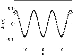
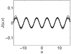
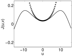
Figure 5: Comparison of the asymptotic approximation (117) (open circles) with the exact two-dimensional Bessel function $J_{n}^{1,2}(u,v)$ (full line) for $n=30$. Left: Case (i) for $v=64$ using eq. (104). Middle: Case (ii) with $v=-12$ using eq. (117). Right: Case (ii) with $v=+12$ using eq. (121)

The asymptotic approximations (104) and (117) provide explicit estimates for the nodal lines of $J_{n}^{1,2}(u,v)$. For $n<2|v|$ we find

$$u\sqrt{\frac{1}{2}-\frac{n}{4v}}=\left\{\begin{array}[]{ll}(2j+1)\frac{\pi}{2}&n\mbox{ even}\\[5.69054pt] j\pi&n\mbox{ odd}\end{array}\right.\quad,\quad j=0,\,\pm 1,\,\pm 2,\ldots$$ (125)

and for $n>2|v|$ we have for $v<0$ zeros at

$$u\,\sqrt{\frac{1}{2}-\frac{n}{4v}}=\big{(}2j+n\big{)}\frac{\pi}{2}\quad,\quad j=0,\,\pm 1,\,\pm 2,\ldots\,.$$ (126)

These results are, of course, in agreement with the zeros observed in fig. 5.

4.3 Large arguments $u$, $v$ and large index $n$

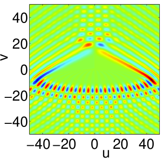
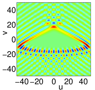
Figure 6: Color map of the two-dimensional Bessel functions $J_{n}^{1,2}(u,v)$ for $n=29$ (left) and $n=30$ (right). Note the different symmetries of these functions. Their overall structure can be explained by means of the bifurcation set shown in fig. 7.

As an example of the structure of the two-dimensional Bessel functions for large indices, fig. 6 shows $J_{n}^{1,2}(u,v)$ for $n=29$ and $n=30$. These functions look quite similar, they are clearly distinguished, however, by their symmetry property $J_{n}^{1,2}(-u,v)=(-1)^{n}J_{n}^{1,2}(u,v)$ (see eq. (28)), i.e. $J_{30}^{1,2}$ is even and $J_{29}^{1,2}$ is odd with respect to a reflection $u\rightarrow-u$. Therefore $J_{29}^{1,2}$ vanishes on the $v$-axis, $J_{29}^{1,2}(0,v)=0$. The function $J_{30}^{1,2}$ is symmetric on the $v$-axis: $J_{n}^{1,2}(0,-v)=J_{n}^{1,2}(0,v)$ (see eq. (37)), despite of the apparent asymmetry with respect to the reflection $v\rightarrow-v$.

In additions to the oscillatory pattern in the four sectors, we observe a region close to the center where the values of the Bessel functions are small. This pattern can again be explained by a consideration of the asymptotic limit where both arguments and the index $n$ are large using

$$g(t)=u\sin pt+v\sin qt-nt$$ (127)

in the stationary phase approximation (72). The stationary points $t_{s}$ are determined by

$$g^{\prime}(t_{s})=pu\cos pt_{s}+qv\cos qt_{s}-n=0\,.$$ (128)

The zeros of the second derivative

$$g^{\prime\prime}(t)=-p^{2}u\sin pt-q^{2}v\sin qt$$ (129)

appearing in the denominator of (72) determine the bifurcation set of these solutions.

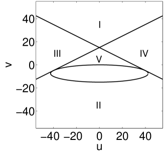
Figure 7: Bifurcation curves of the stationary points for the two-dimensional Bessel function $J_{30}^{1,2}(u,v)$.

Restricting ourselves again to the case $(p,q)=(1,2)$ these equations simplify and can be solved in closed form:

$$g^{\prime}(t_{s}) = u\cos t_{s}+2v\cos 2t_{s}-n=0$$ (130)

with solutions

$$c_{\pm}=\cos t_{s}=-\frac{u}{8v}\pm\sqrt{\Big{(}\frac{u}{8v}\Big{)}^{2}+\frac{1}{2}+\frac{n}{4v}\,}$$ (131)

(here again each solution $c_{\pm}$ implies two stationary points $t_{s}$ because of the symmetry of the cosine function). The bifurcation set – the skeleton of the Bessel function – is found when

$$g^{\prime\prime}(t_{s})=-u\sin t_{s}-4v\sin 2t_{s}=0$$ (132)

is satisfied in addition to (130). Eliminating $t_{s}$ we find the solutions

$$v=(n\pm u)/2$$ (133)

(note that for $|u|\gg n$ these straight lines agree with the ones stated above in eq. (81)) and the ellipse

$$\frac{16(v+n/4)^{2}}{n^{2}}+\frac{u^{2}}{2n^{2}}=1$$ (134)

centered at  $(u,v)=(0,-n/4)$  with half axes $\sqrt{2}\,n$ and $n/4$. Inside this ellipse the stationary points (131) are complex, outside they are real. A brief calculation furthermore shows that the straight lines (133) are tangential to the ellipse (134). This bifurcation set is shown in fig. 7. In the upper sector (I) between the bifurcation lines we have $-1<c_{\pm}<+1$, as well as in the lower sector (II) outside the ellipse. Hence we have four real solutions $t_{s}$ in these regions and a corresponding oscillatory pattern. In the right sector (IV) two of these solutions become complex because of $|c_{+}|>1$ and similarly in the left hand sector (III) with $|c_{-}|>1$. In the triangular segment (V) in the lower sector above the ellipse, we have $|c_{+}|>1$ and $|c_{-}|>1$ and therefore no real stationary points. In the elliptic region with complex valued stationary points, the Bessel function is damped but still oscillatory. An example is shown in fig. 5 (right hand side) which shows a cut through the Bessel function $J_{30}^{1,2}(u,v)$ shown in fig. 6 for $v=-12$ close to the elliptic bifurcation curve. A cut at $v=64$ (left hand side) shows the oscillations in region (I). Note that the semiclassical approximations shown in fig. 5 are the simplified versions developed in section 4.2. A more refined semiclassical treatment along the lines discussed above will provide a much better agreement for larger values of $u$ (compare also the treatment in [5]).

References

- [1] P. Appell, C. R. Acad. Sci. 160 (1915) 419
- [2] J. Pérès, C. R. Acad. Sci. 161 (1915) 160
- [3] A. I. Nikishov and V. I. Ritus, Sov. Phys. JETP 10 (1964) 529
- [4] A. Wasiljeff, Z. angew. Math. Phys. 20 (1969) 389
- [5] H. R. Reiss, Phys. Rev. A 22 (1980) 1786
- [6] W. Becker, R. R. Schlicher, and M. O. Scully, J. Phys. B 19 (1986) L785
- [7] W. Becker, R. R. Schlicher, M. O. Scully, and K. Wódkiewicz, J. Opt. Soc. Am. B 4 (1987) 743
- [8] G. Dattoli, C. Chiccoli, S. Lorenzutta, G. Maino, M. Richetta, and A. Torre, J. Math. Phys. 33 (1992) 25
- [9] W. A. Paciorek and G. Chapuis, Acta Cryst. A50 (1994) 194
- [10] H.R. Reiss and V.P. Krainov, J. Phys. A 36 (2003) 5575
- [11] F. Keck and H. J. Korsch, J. Phys. A 35 (2002) L105
- [12] H. J. Korsch and S. Mossmann, Phys. Lett. A 317 (2003) 54
- [13] J. Bauer, J. Phys. A 38 (2005) 521
- [14] G. Dattoli and A. Torre, Theory and Applications of Generalized Bessel Functions, Aracne Editrice, Rome, 1996
- [15] A. Klumpp, D. Witthaut, and H. J. Korsch, quant-ph/0608217 (2006)
- [16] G. Dattoli, L. Giannessi, L. Mezi M, and A. Torre, Nuovo Cim. 105B (1990) 327
- [17] G. Dattoli, A. Torre, S. Lorenzutta, G. Maino, and C. Chiccoli, Nuovo Cim. 106 B (1991) 21
- [18] G. Dattoli, C. Chiccoli, S. Lorenzutta, G. Maino, M. Richetta, and A. Torre, Nuovo Cim. 106 B (1991) 1159
- [19] S. Lorenzutta, G. Maino, G. Dattoli, A. Torre, and C. Chiccoli, Rendiconti di Matematica, Serie VII 15 (1995) 405
- [20] L. J. Mordell, Diophantine Equations, Academic Press, London and New York, 1969
- [21] G. Dattoli, A. Torre, S. Lorenzutta, and G. Maino, Comp. Math. Applic. 32 (1998) 117
- [22] G. Dattoli, Integral Transforms and Special Functions 15 (2004) 303
- [23] G. Dattoli, C. Cesarano, and S. Sacchetti, Georgian Math. J. 9 (2002) 473
- [24] G. Dattoli, C. Mari, A. Torre, C. Chiccoli, S. Lorenzutta, and G. Maino, J. Sci. Comput. 7 (1992) 175
- [25] J. E. Marsden, Basic Complex Analysis, Freeman, New York, 1987
- [26] C. Leubner, Phys. Rev. A 23 (1981) 2877
- [27] M. Abramowitz and I. A. Stegun, Handbook of Mathematical Functions, Dover Publications, Inc., New York, 1972
- [28] J. R. Stine and R. A. Marcus, J. Chem. Phys. 59 (1973) 5145