Quantum sensitivity limit of a Sagnac hybrid interferometer based on slow-light propagation in ultra-cold gases

Abstract

The light–matter-wave Sagnac interferometer based on ultra-slow light proposed recently in (Phys. Rev. Lett. 92, 253201 (2004)) is analyzed in detail. In particular the effect of confining potentials is examined and it is shown that the ultra-slow light attains a rotational phase shift equivalent to that of a matter wave, if and only if the coherence transfer from light to atoms associated with slow light is associated with a momentum transfer and if an ultra-cold gas in a ring trap is used. The quantum sensitivity limit of the Sagnac interferometer is determined and the minimum detectable rotation rate calculated. It is shown that the slow-light interferometer allows for a significantly higher signal-to-noise ratio as possible in current matter-wave gyroscopes.

I Introduction

In contrast to inertial motion, rotation of an object is absolute in the sense that it can be defined intrinsically, i.e. independent of any inertial frame of reference. Rotation can be detected e.g. by means of the Sagnac effect Sagnac (1913), i.e. the relative phase shift $\Delta\phi_{\rm rot}$ of counterpropagating waves in a ring interferometer of area $\mathbf{A}$ attached to the laboratory frame rotating with angular velocity $\mathbf{\Omega}$.

$$\Delta\phi_{\rm rot}=\frac{4\pi}{\lambda v}\mathbf{\Omega}\cdot\mathbf{A},$$ (1)

where $\lambda$ is the wavelength and $v$ the phase velocity of the wave. Depending on the nature of the wave phenomena employed, one distinguishes two basic types of Sagnac interferometer: laser Post (1967); Chow et al. (1985); Stedman (1997) and matter-wave gyroscopes Bongs and Sengstock (2004). The Sagnac phase shift per unit area in a matter-wave device exceeds that of laser-based gyroscopes by the ratio of rest energy per particle to photon energy $mc^{2}/\hbar\omega$ which for alkali atoms and optical photons is of the order of $10^{11}$ Scully and Zubairy (1997); Page (1975). Despite this very large number, matter-wave gyroscopes have only recently reached the short-time sensitivities of laser based devices Gustavson et al. (1997); McGuirk et al. (2000). This has mainly two reasons: First of all, laser-based gyroscopes, especially fiber-optics interferometer, can have a much larger area than matter-wave systems Culshaw (2006). Secondly the large flux of photons achievable in optical systems leads to a much lower shot-noise level as compared to matter-wave devices Chow et al. (1985); Kasevich (2002). Thus in order to make full use of the much larger rotational sensitivity per unit area in a matter-wave device one needs to find ways to increase (i) the interferometer area and (ii) the particle flux. While a substantial increase of the interferometer area in matter-wave devices is difficult, the use of novel cooling techniques has lead to high-flux atom sources which improved the performance of atom interferometers Orzel et al. (2001); Bongs and Sengstock (2004). With particle throughputs which can now reach $10^{8}$ s^-1 as compared to a few atoms per second in the first atomic interferometers, the noise level is however still much higher than that achievable in fiber optics gyroscopes with photon counting rates on the order of $10^{16}$ s^-1 Kasevich (2002); Bongs and Sengstock (2004). Continuously loaded Bose-Einstein condensates (BEC) could provide a source for coherent atoms with larger flux values, and substantial progress has been made in this direction over the past few years Chikkatur et al. (2002).

We recently proposed a light–matter-wave hybrid interferometer based on slow-light propagation in ultra-cold gases of 3-level atoms Zimmer and Fleischhauer (2004). We argued that this interferometer would combine the large rotational phase shift of matter-wave systems with the large area typical for optical gyroscopes. To this end the simultaneous coherence and momentum transfer associated with ultra-slow light in cold atomic gases with electromagnetically induced transparency (EIT) Fleischhauer et al. (2005) was utilized. As the reduction of the group velocity of light in 3-level EIT media is based on the change of character of the dressed eigenmodes of the systems from electromagnetic excitations to atomic Raman excitations Fleischhauer and Lukin (2000), light waves can coherently be transformed into matter waves. These matter waves pick up a Sagnac phase shift per unit area which is orders of magnitude larger than the corresponding value for electromagnetic fields.

In the present paper we present a detailed theoretical description of the light-matter-wave hybrid interferometer. In particular we discuss the effect of confining potentials for the atoms. We find that in contrast to the case of an infinitely extended medium or of periodic boundary conditions, which have been assumed in Zimmer and Fleischhauer (2004), the wavefunctions of all three internal states acquire the same matter-wave contribution to the Sagnac phase when in motional equilibrium with a trapping potential Hendriks and Nienhuis (1990). As a consequence the matter-wave contribution to the rotational phase shift vanishes. Only if periodic boundary conditions for the ground-state wavefunction can be maintained a nonvanishing matter-wave contribution to the rotational phase shift emerges. This can be realized e.g. in a circular-waveguide BEC Gupta et al. (2005); Arnold et al. (2006). The need for a circular atomic waveguide puts more stringent restrictions to the possible interferometer area then assumed in Zimmer and Fleischhauer (2004) and thus partially invalidates the advantages of the hybrid interferometer stated in that paper. We will show however, that despite this restriction the minimum detectable rotation rate at the shot-noise limit can exceed the current state of the art. It corresponds to that of a matter-wave gyroscope with a rather large particle flux given by the high density of the ultra-cold gas, e.g. a BEC, multiplied by the recoil velocity. To determine the quantum sensitivity limit of the hybrid interferometer the saturation of the Sagnac phase shift with the probe-light intensity as well as probe-field absorption will be taken into account. It will be shown that the Sagnac phase attains a maximum value for a certain value of the probe power. Optimum parameter values for a maximum signal-to-noise ratio (SNR) will be determined and the minimum detectable rotation rate $\Omega_{\rm min}$ per unit area derived.

II Dynamics in the rotating frame

An intrinsic sensor attached to the laboratory frame detects the rotation of the frame without any reference to some other, non-rotating frame of reference. Thus it is most natural to describe this system from the point of view of a co-rotating observer. We will give here a microscopic description of the gyroscope which consists of an ensemble of three-level atoms with internal states $|1\rangle$, $|2\rangle$, and $|3\rangle$ in a ring interferometer, coupled by two laser fields with (complex) Rabi frequencies $\Omega_{c}$ and $\Omega_{p}$ in a Raman configuration as shown in Fig. 1 (left). The probe field $\Omega_{p}$ is assumed to propagate clockwise and counter-clockwise with respect to the rotation axis $\mathbf{e}_{z}$ with its beam path bound to a circle of radius $R$ as depicted in Fig. 1 (right). The control field $\Omega_{c}$, which is assumed to have a much larger Rabi frequency than the probe field, propagates in a different direction such that the corresponding wavevectors are (nearly) perpendicular. The ensemble as well as the laser sources are attached to the laboratory frame rotating with angular velocity $\mathbf{\Omega(t)}=\Omega(t)\mathbf{e}_{z}$ Dufour and Prunier (1937). The center-of-mass motion of the atoms shall also be confined to the periphery of the circular loop. Furthermore, it is assumed that $|\Omega|R\ll c$ such that non-relativistic quantum mechanics applies.

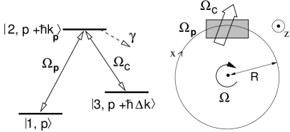
Figure 1: (left) atomic level scheme. $p$ denotes the momentum of the atoms and $k_{p}$ the wavevector of the probe-field along the periphery ($x$) of the circular loop depicted in the right part of the figure. $k_{c}^{\parallel}$ in the component of the control-field wavevector along $x$, and $\Delta k=k_{p}-k_{c}^{\parallel}$. (right) Schematic set-up of the hybrid Sagnac interferometer with vapor cell (grey box) attached to the rotating frame with angular velocity ${\Omega}$.

Under conditions of two-photon resonance, the control field $\Omega_{c}$ generates EIT for the probe field associated with a substantial reduction of its group velocity Hau et al. (1999); Budker et al. (1999); Kash et al. (1999). The group velocity reduction which is due to the coupling of the probe light to the atomic Raman coherence corresponds in a quasi-particle picture to the formation of so-called dark-state polaritons, a superposition of light and matter degrees of freedom Fleischhauer and Lukin (2000); Matsko et al. (2001). The smaller the group velocity the larger the contribution of the matter component in the polariton.

The atoms are here described in second quantization by three Schrödinger fields $\hat{\Psi}_{1}(\textbf{r},t)$, $\hat{\Psi}_{2}(\textbf{r},t)$, and $\hat{\Psi}_{3}(\textbf{r},t)$ corresponding to the three internal states. In order to describe the propagation of the probe light and the three matter-wave fields in the co-rotating frame, we need to transform the Hamiltonian of the system into the rotating frame.

As the starting point we choose the standard atom-light interaction Hamiltonian of quantum optics in Coulomb gauge and after the Power-Zienau-Wolley transformation Cohen-Tannoudji et al. (1997). Adding the free Hamiltonian of a 3-component non-relativistic Schrödinger field, the Hamiltonian reads in a non-rotating frame

$$\hat{H}=\hat{H}^{(A)}+\hat{H}^{(F)}+\hat{H}^{(I)}$$

$$\enspace=\sum_{\mu}\int\!{\rm d}^{3}r\,\hat{\Psi}_{\mu}^{\dagger}({\mathbf{r}})\biggl{[}-\frac{\hbar^{2}}{2m}{\boldsymbol{\nabla}}^{2}+\hbar\omega_{\mu}+V_{\mu}^{\rm ext}({\mathbf{r}},t)\,\biggr{]}\hat{\Psi}_{\mu}({\mathbf{r}})$$

$$\enspace+\frac{\epsilon_{0}}{2}\int{\rm d}^{3}r\,\left[\left(\frac{\hat{\mathbf{\Pi}}({\mathbf{r}})}{\epsilon_{0}}\right)^{2}+c^{2}\left({\boldsymbol{\nabla}}\times\hat{\mathbf{A}}_{\bot}({\mathbf{r}})\right)^{2}\right]$$ (2)

$$\enspace+\sum_{\mu,\nu}\int{\rm d}^{3}r\,\hat{\Psi}^{\dagger}_{\mu}({\mathbf{r}})\left[{\mathbf{d}}_{\mu\nu}\cdot\left(\hat{{\mathbf{\Pi}}}({\mathbf{r}})-{\mathbf{E}}_{\rm ext}({\mathbf{r}},t))\right)\right]\hat{\Psi}_{\nu}({\mathbf{r}}).$$

$\hat{H}^{\rm(A)}$ describes the motion of atoms in an external, possibly state- and time-dependent trapping potential $V^{\rm ext}_{\mu}(\mathbf{r},t)$, $E_{\mu}=\hbar\omega_{\mu}$ is the energy of atoms in state $|\mu\rangle$. The free Hamiltonian of the radiation field is denoted by $\hat{H}^{\rm(F)}$, where $\hat{\mathbf{A}}_{\bot}({\mathbf{r}})$ is the transverse part of the vector potential and $\hat{\mathbf{\Pi}}({\mathbf{r}})$ its conjugate momentum. Finally $\hat{H}^{\rm(I)}$ describes the interaction of the atoms with the quantized electromagnetic field and additional external fields in dipole approximation, where ${\mathbf{d}}_{\mu\nu}$ is the vectorial dipole matrix element between internal states $|\mu\rangle$ and $|\nu\rangle$. For notational simplicity we will drop the subscript ${}^{\prime\prime}\bot^{\prime\prime}$ in the following.

The transition to a frame rotating with angular velocity ${\mathbf{\Omega}}(t)$ is done via the unitary transformation

$$U(t)=\exp\left(-\frac{\rm i}{\hbar}\int_{t_{0}}^{t}\!\!{\rm d}\tau\,\,{\mathbf{\Omega}}(\tau)\cdot\hat{{\mathbf{L}}}\right),$$ (3)

where $\hat{{\mathbf{L}}}$ is the total angular momentum operator of light and matter. By choosing ${\mathbf{\Omega}}=\Omega\,{\mathbf{e}}_{z}$ we restrict ourselves to a rotation about the fixed $z$-axis. In this case only the vector component parallel to that axis, i. e.

$$\hat{L}_{z} =\hat{L}_{z}^{(\rm A)}+\hat{L}_{z}^{(\rm F)}$$

$$=\frac{\hbar}{\rm i}\sum_{\mu}\int\!\!{\rm d}^{3}r\,\hat{\Psi}_{\mu}^{\dagger}\partial_{\varphi}\hat{\Psi}_{\mu}$$ (4)

$$-\frac{1}{2}\sum_{j}\int\!\!{\rm d}^{3}r\,\left[\hat{{\Pi}}_{j}(\partial_{\varphi}\hat{{A}}_{j})+(\partial_{\varphi}\hat{{A}}_{j})\hat{{\Pi}}_{j}\right]$$

is relevant. In eq. (4) the index $\mu$ denotes the three internal states and the index $j$ the three spatial dimensions. The Hamiltonian in the rotating frame is hence given by

$$\hat{H}_{\rm rot}=U(t)\,\hat{H}\,U^{\dagger}(t)+{\Omega}(t)\hat{L}_{z}.$$ (5)

Since $\hat{L}_{z}^{(\rm A)}$ and $\hat{L}_{z}^{(\rm F)}$ commute, the unitary transformation eq. (3) can be decomposed into two operators which act on the matter-wave and on the electromagnetic field respectively. One finds

$$\hat{H}_{\rm rot}^{\rm(A)}=\Omega(t)\hat{L}_{z}^{\rm(A)}+$$ (6)

$$+\sum_{\mu}\int{\rm d}^{3}r^{\prime}\hat{\Psi}^{\dagger}_{\mu}({\mathbf{r}}^{\prime})\biggl{[}-\frac{\hbar^{2}}{2m}{\boldsymbol{\nabla}^{\prime}}^{2}+\hbar\omega_{\mu}+V^{\rm ext}_{\mu}\left({\mathbf{r}}^{\prime}\right)\biggr{]}\hat{\Psi}_{\mu}({\mathbf{r}}^{\prime}),$$

$$\hat{H}_{\rm rot}^{\rm(F)}=\Omega(t)\hat{L}_{z}^{\rm(F)}+\hat{H}_{0}^{(F)}$$ (7)

$$+\sum_{\mu,\nu}\int{\rm d}^{3}r^{\prime}\,\hat{\Psi}^{\dagger}_{\mu}({\mathbf{r}^{\prime}})\left[{\mathbf{d}}_{\mu\nu}\cdot\left(\hat{{\mathbf{\Pi}}}({\mathbf{r}^{\prime}})-{\mathbf{E}}_{\rm ext}({\mathbf{r}^{\prime}},t)\right)\right]\hat{\Psi}_{\nu}({\mathbf{r}^{\prime}}).$$

Here the prime denotes that the variables are given with respect to the rotating coordinates

$${\mathbf{r}}^{\prime} = {\mathbf{r}}+\int_{t_{0}}^{t}\!\!{\rm d}\tau\,{\mathbf{e}}_{\varphi}\,R\,\Omega(\tau),$$ (8)

with $R$ being the distance from the rotation axis. For all field operators $\hat{\mathbf{F}}\in\{\hat{\Psi},\hat{\mathbf{\Pi}},\hat{\mathbf{A}}\}$ holds:

$$U\hat{\mathbf{F}}({\mathbf{r}})U^{\dagger}=\hat{\mathbf{F}}\Bigl{(}{\mathbf{r}}+\int_{t_{0}}^{t}\!\!{\rm d}\tau\,\,{\mathbf{e}}_{\varphi}\,R\,\Omega(\tau)\Bigr{)}.$$ (9)

The center-of-mass dynamics of the matter-wave fields is then governed by the following Heisenberg equations of motion in the co-rotating frame

$${\rm i}\hbar\Bigl{(}\partial_{t} +\,\,\Omega(t)\,\partial_{\varphi}\Bigr{)}\hat{\Psi}_{\mu}({\mathbf{r}}^{\prime},t)=$$ (10)

$$=\biggl{[}-\frac{\hbar^{2}}{2m}{\boldsymbol{\nabla}}^{\prime\,2}+\hbar\omega_{\mu}+V^{\rm ext}_{\mu}({\mathbf{r}}^{\prime})\biggr{]}\hat{\Psi}_{\mu}({\mathbf{r}}^{\prime},t)$$

$$+\sum\limits_{\nu}{\mathbf{d}}_{\mu\nu}\cdot\left(\hat{\mathbf{\Pi}}({\mathbf{r}}^{\prime})-{\mathbf{E}}_{\rm ext}({\mathbf{r}}^{\prime},t)\right)\hat{\Psi}_{\nu}({\mathbf{r}}^{\prime},t).$$ (11)

Correspondingly the equations of motion for the conjugate momentum $\hat{{\mathbf{\Pi}}}$ and the transversal vector potential $\hat{\mathbf{A}}$ read

$$\Bigl{(}\partial_{t}+\Omega(t)\partial_{\varphi^{\prime}}\Bigr{)}\hat{{\mathbf{\Pi}}}({\mathbf{r}}^{\prime},t)=-\frac{1}{\mu_{\rm 0}}{\boldsymbol{\nabla}}^{\prime}\times({\boldsymbol{\nabla}}^{\prime}\times\hat{{\mathbf{A}}}({\mathbf{r}}^{\prime},t)),$$ (12)

and

$$\Bigl{(}\partial_{t}+\Omega(t)\partial_{\varphi^{\prime}}\Bigr{)}\hat{{\mathbf{A}}}({\mathbf{r}}^{\prime},t)=\frac{1}{\epsilon_{\rm 0}}\hat{{\mathbf{\Pi}}}({\mathbf{r}}^{\prime},t)+\frac{1}{\epsilon_{\rm 0}}\hat{{\mathbf{P}}}({\mathbf{r}}^{\prime},t).$$ (13)

In eq. (13) we have introduced the transversal polarization $\hat{{\mathbf{P}}}({\mathbf{r}},t)=\sum_{\mu,\nu}\hat{\Psi}^{\dagger}_{\mu}({\mathbf{r}},t)\,{\mathbf{d}}_{\mu\nu}\hat{\Psi}_{\nu}({\mathbf{r}},t)$. It is immediately obvious that the transformation to the rotating frame just amounts to the replacement $\partial_{t}\,\longrightarrow\partial_{t}+\Omega(t)\,\partial_{\varphi}$. For notational simplicity we will omit in the following the prime that indicates rotating coordinates.

As we work in the Coulomb gauge we have $\hat{{\mathbf{\Pi}}}({\mathbf{r}},t)=-\hat{\mathbf{D}}({\mathbf{r}},t)$ Cohen-Tannoudji et al. (1997). Using this and $\hat{{\mathbf{D}}}({\mathbf{r}})=\epsilon_{\rm 0}\hat{{\mathbf{E}}}({\mathbf{r}})+\hat{{\mathbf{P}}}({\mathbf{r}})$ we find for the wave equation of the electric field in the rotating frame

$$\left[\Bigl{(}\partial_{t}+\Omega(t)\partial_{\varphi}\Bigr{)}^{2}-\,c^{2}\,\bigtriangleup\right]\hat{{\mathbf{E}}}({\mathbf{r}},t)$$

$$\qquad\qquad=\frac{1}{\epsilon_{0}}\Bigl{(}\partial_{t}+\Omega(t)\partial_{\varphi}\Bigr{)}^{2}\hat{{\mathbf{P}}}({\mathbf{r}},t).$$ (14)

We now introduce slowly varying variables for the transverse field as well as polarization by $\hat{{\mathbf{E}}}({\mathbf{r}},t)=\hat{\boldsymbol{\mathcal{E}}}^{(+)}(x,r_{\bot},t)\,e^{-{\rm i}(\omega_{p}t-k_{p}x)}+h.a.$ and $\hat{\mathbf{P}}({\mathbf{r}},t)=\hat{\boldsymbol{\mathcal{P}}}^{(+)}(x,r_{\bot},t)\,e^{-{\rm i}(\omega_{p}t-k_{p}x)}+h.a.\,$, where $x=R\varphi$ is the arclength on the circle. Restricting ourselves to propagation along the periphery of the interferometer we find within the slowly varying envelope approximation and by neglecting terms ${\mathcal{O}}(\Omega\,R/c)$

$$\Bigl{[}\partial_{t}+c\partial_{x}+{\rm i}k_{\rm p}\Omega R\Bigr{]}\,\hat{\boldsymbol{\mathcal{E}}}^{(+)}(x,t)=-\frac{{\rm i}\,\omega_{\rm p}}{2\,\epsilon_{0}}\hat{\boldsymbol{\mathcal{P}}}^{(+)}(x,t).$$ (15)

The term proportional to the rotation rate $\Omega$ is responsible for the rotation induced Sagnac phase shift in the pure light case, i. e. without any influence from the medium polarization. As shown in Zimmer and Fleischhauer (2004) and in the next section the polarization leads to an additional phase shift.

Introducing also slowly varying amplitudes for the matter fields $\hat{\Psi}_{1}=\hat{\Phi}_{1}$, $\hat{\Psi}_{2}=\hat{\Phi}_{2}\,e^{-{\rm i}(\omega_{p}t-k_{p}x)}$ and $\hat{\Psi}_{3}=\hat{\Phi}_{3}\,e^{-{\rm i}(\Delta\omega t-\Delta kx)}$ with $\Delta\omega=\omega_{p}-\omega_{c}$ and $\Delta k=k_{p}-k^{\parallel}_{c}$, where $k^{\parallel}_{c}$ is the wavevector projection of the control field onto the $x$-axis, we find

$$\Bigl{(}{\mathcal{D}}_{\rm 1}-V_{1}(x)\Bigr{)}\hat{\Phi}_{1} =\hbar\Omega_{p}^{*}\hat{\Phi}_{2},$$ (16)

$$\Bigl{(}{\mathcal{D}}_{\rm 2}+\hbar(\Delta_{2}-k_{p}\Omega R-V_{2}(x))\Bigr{)}\hat{\Phi}_{2} =\hbar\Omega_{p}\hat{\Phi}_{1}$$

$$+\hbar\Omega_{c}\hat{\Phi}_{3},$$ (17)

$$\Bigl{(}{\mathcal{D}}_{\rm 3}-V_{3}(x)+\hbar(\Delta_{3}-\eta k_{p}\Omega R)\Bigr{)}\hat{\Phi}_{3} =\hbar\Omega_{c}^{*}\hat{\Phi}_{2}$$ (18)

with

$${\mathcal{D}}_{\mu}={\rm i}\,\hbar\,\partial_{t}+\frac{\hbar^{2}\partial^{2}_{x}}{2m}+{\rm i}\,\hbar\,(\Omega R+\eta_{\mu}v_{\rm rec})\partial_{x}.$$ (19)

Here we have used the definitions $\Delta_{2}=\omega_{p}-\omega_{2}-\omega_{\rm rec}$ and $\Delta_{3}=\Delta\omega-\omega_{3}-\eta^{2}{\omega_{\rm rec}}$ for the one- and two-photon-detuning including the recoil shift ($\omega_{\rm rec}=\hbar k_{p}^{2}/2m$). $v_{\rm rec}=\hbar k_{p}/m$ is the single-photon recoil velocity. We have also introduced the dimensionless parameter $\eta=\Delta k/k_{p}$ which describes the momentum transfer from the light fields to the atoms in state $|3\rangle$ as well as the abbreviation $\eta_{\mu}=\delta_{\mu,2}+\eta\,\delta_{\mu,3}$. Finally the definitions $\Omega_{p,c}=-{\mathbf{d}}_{p,c}\cdot{\mathbf{E}}^{(p,c)}_{\rm ext}$ for the probe and control-field Rabi frequencies were applied. The shortened wave equation (15) and the matter-wave field equations (16)-(18) are the basis of the following study of the sensitivity enhancement of the light–matter-wave hybrid Sagnac interferometer.

III Sagnac phase shift and influence of external trapping potentials

In this section we will calculate the stationary Sagnac phase shift for the hybrid interferometer in the perturbative limit of low probe-light intensities. In particular we will analyze the effects of a trap potential which confines the atoms to certain regions in the direction of the interferometer path. For simplicity we assume a constant rotation rate, i.e. $\dot{\Omega}=0$, and consider the stationary state. All atoms are assumed to be initially, i. e. before applying any probe-field, in the internal state $|1\rangle$. This amounts to set $\hat{\Phi}_{2}^{(0)}(t=0)=\hat{\Phi}_{3}^{(0)}(t=0)=0$. In the perturbative limit of small probe field intensity, $\hat{\Phi}_{1}$ is not changed by the atom-light interaction, i. e. it obeys the equation

$$\Bigl{(}\frac{\hbar^{2}\partial_{x}^{2}}{2m}+{\rm i}\hbar\Omega R\partial_{x}+\left(\epsilon_{1}-V_{1}(x)\right)\Bigr{)}\hat{\Phi}_{1}^{(0)}(x)=0,$$ (20)

where $\epsilon_{1}$ is the energy in the stationary state. Assuming $|\Omega_{c}|\gg|\Delta_{2}|,k_{p}|\Omega|R,|V_{2}(x)|/\hbar$ one finds in first order from eq. (17)

$$\hat{\Phi}_{3}^{(1)}(x)=-\frac{\Omega_{p}(x)}{\Omega_{c}}\hat{\Phi}_{1}^{(0)}(x),$$ (21)

which amounts to an adiabatic elimination of the excited state. Using this and eq. (18) we find

$$\hat{\Phi}_{2}^{(1)}= \,\eta\,k_{p}\frac{\Omega R}{|\Omega_{c}|^{2}}\hat{\Phi}_{1}^{(0)}\Omega_{p}(x)-\frac{1}{|\Omega_{c}|^{2}}\left[\frac{\hbar}{2m}\partial_{x}^{2}\right.$$

$$\left.+{\rm i}\,(\Omega R+\eta v_{\rm rec})\partial_{x}+\frac{\epsilon_{3}-V_{3}(x)}{\hbar}\right]\hat{\Phi}_{1}^{(0)}\Omega_{p}(x)$$ (22)

$$= \enspace\eta\,\frac{\hat{\Phi}_{1}^{(0)}}{|\Omega_{c}|^{2}}\Bigl{(}{\rm i}v_{\rm rec}\partial_{x}\ln{\hat{\Phi}}_{1}+k_{p}\Omega R\Bigr{)}\Omega_{p}(x)$$

$$-\frac{\hat{\Phi}_{1}^{(0)}}{|\Omega_{c}|^{2}} \left[\frac{\hbar\partial_{x}^{2}}{2m}+{\rm i}\Bigl{(}\Omega R+\eta v_{\rm rec}-{\rm i}\frac{\hbar}{m}\partial_{x}\ln{\hat{\Phi}}_{1}^{(0)}\Bigr{)}\partial_{x}\right]\Omega_{p}(x),$$

where we have in addition assumed two-photon resonance, i. e. $\Delta_{3}=0$. In deriving the second equation, which is useful for later discussions, we have made use of eq. (20) and assumed equal trapping potentials for the internal states $V_{1}=V_{3}$. Furthermore an unimportant constant energy term proportional to $\epsilon_{1}-\epsilon_{3}$ has been dropped. One recognizes that the fields $\hat{\Phi}_{2}^{(1)}$ and $\hat{\Phi}_{3}^{(1)}$ and thus the medium polarization in first order of perturbation follow straight forwardly from the solution of eq.(20).

We will now consider two cases. In the first case no confining potential for atoms in state $|1\rangle$ is assumed, which is equivalent to translational invariance on a ring. In the second case, discussed later, a trapping potential in the longitudinal direction $x$ is taken into account. We will see that both cases lead to quite different results.

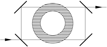
Figure 2: Set-up of a Sagnac interferometer with ring-shaped trap configuration supporting a superfluid ultra-cold gas (BEC). The symmetric interferometer set-up allows for a distinction of rotational from linear acceleration.

III.1 Periodic boundary conditions in state $|1\rangle$

Let us consider the case that atoms in state $|1\rangle$ do not experience any confining potential in the $x$-direction. Since $x$ is the coordinate along the periphery of the interferometer, this amounts to considering a ring-trap configuration with periodic boundary conditions $\hat{\Phi}_{1}^{(0)}(x+2\pi R)=\hat{\Phi}_{1}^{(0)}(x)$. The principle set-up is shown in Fig. (2). With $V_{1}(x)\equiv 0$, eq. (20) has the eigensolutions

$${\hat{\Phi}}_{1n}^{(0)}(x)=\hat{\Phi}_{0}\,\exp\left\{i\frac{n}{R}x\right\}\qquad\epsilon_{n}=n\hbar\Omega+\frac{n^{2}\hbar^{2}}{2mR^{2}}$$

where ${\hat{\Phi}}_{0}$ is a constant. Taken as a continuous function of $n$, the spectrum $\epsilon(n)$ is a parabola with minimum at

$$n_{\rm min}=-\frac{m\Omega R^{2}}{\hbar}.$$ (23)

This is illustrated in Fig. 3. Taking into account that $n$ must be a positive or negative integer, the state with the lowest energy corresponds to $n=0$ as long as $|n_{\rm min}|<1/2$, i.e. as long as the Sagnac phase shift per round trip is smaller than $\pi$.

III.1.1 Bose-Einstein condensate

We now assume that only the lowest motional energy state in the internal state $|1\rangle$ is initially excited, e.g. a Bose-Einstein condensate in the ring trap. In this case there is a uniform phase over the whole ring and we can set $\hat{\Phi}_{1}^{(0)}(x)=\hat{\Phi}_{0}$. It is important to note that the particles in the ground state do not attain a rotational phase shift in this case. This yields with eq. (22)

$$\hat{\Phi}_{2}^{(1)}(x)=\eta k_{p}\frac{\Omega R}{|\Omega_{c}|^{2}}{\hat{\Phi}}_{0}\,\Omega_{p}(x)$$ (24)

$$\quad-\frac{{\rm i}(\Omega R+\eta v_{\rm rec}){\hat{\Phi}}_{0}}{|\Omega_{c}|^{2}}\partial_{x}\,\Omega_{p}(x)-\frac{1}{|\Omega_{c}|^{2}}{\hat{\Phi}}_{0}\frac{\hbar}{2m}\partial_{x}^{2}\,\Omega_{p}(x).$$

Substituting the expressions for $\hat{\Phi}_{2}^{(1)}$ and $\hat{\Phi}_{1}^{(0)}$ into the stationary, shortened wave equation, eq.(15), for the expectation value of the probe-field expressed in terms of $\Omega_{p}$,

$$\Bigl{(}c\partial_{x}+{\rm i}k_{p}\Omega R\Bigr{)}\Omega_{p}(x)=-{\rm i}g^{2}\Bigl{\langle}{\hat{\Phi}}_{1}^{(0)\dagger}(x){\hat{\Phi}}_{2}^{(1)}(x)\Bigr{\rangle}$$ (25)

where $g=d_{12}\sqrt{\omega_{p}/2\hbar\epsilon_{0}F}$, $d_{12}$ being the dipole matrix element of the $|1\rangle\leftrightarrow|2\rangle$ transition and $F$ the transversal cross-section of the probe-beam, we find

$$\biggl{[}\bigl{\{}c\cos^{2}\theta+(\eta v_{\rm rec}+\Omega R)\sin^{2}\theta\bigr{\}}\partial_{x}-{\rm i}\sin^{2}\theta\frac{\hbar\partial_{x}^{2}}{2m}\biggr{]}\Omega_{p}(x)$$

$$=-{\rm i}k_{p}\Omega R\Bigl{(}\cos^{2}\theta+\eta\sin^{2}\theta\Bigr{)}\Omega_{p}(x).$$ (26)

Here we have introduced the mixing angle $\theta$ through $\tan^{2}\theta=g^{2}\varrho/|\Omega_{c}|^{2}$, where $\varrho=\langle\hat{\Phi}_{0}^{\dagger}\hat{\Phi}_{0}\rangle$ is the density of atoms in state $|1\rangle$. Eq. (26) has a very intuitive interpretation. It describes the propagation of the probe-field with the group velocity

$$v_{\rm gr}=c\,\cos^{2}\theta+\eta\,v_{\rm rec}\,\sin^{2}\theta$$ (27)

in the rotating frame. The propagation of light in an EIT medium is associated with the formation of a dark-state polariton, a superposition of electromagnetic and matter-wave components Fleischhauer and Lukin (2000). If we neglect the atomic motion, the group velocity of this quasi-particle is proportional to the square of the weight factor $\cos\theta$ of the electromagnetic part of the polariton. However, if the coherence transfer from light to atoms is accompanied by a finite momentum transfer of $\eta\,m\,v_{\rm rec}$, there is also a matter-wave contribution to the total group velocity (27). This contribution is again proportional to the square of the weight factor $\sin\theta$ of the matter-wave part. Due to the admixture of the matter wave, the equation of motion (26) attains a term corresponding to the kinetic energy of this component which leads to a dispersive spreading of the probe field along its propagation direction. This term becomes important in the limit $\tan^{2}\theta>\tan^{2}\theta_{\rm crit}\equiv c/v_{\rm rec}$, i.e. when the light wave essentially turns into a propagating spin polarization. The right hand side of eq. (26) describes the light and matter-wave contributions to the rotational phase shift. The matter-wave contribution to the phase shift is non-zero only if there is a finite momentum transfer, i.e. if $\eta\neq 0$. In the limit of small rotation, $|\Omega|R\ll v_{\rm gr}$, which is the case of interest here, eq. (26) can easily be solved. Neglecting the second-order derivative the equation reduces to eq. (11) of ref. Zimmer and Fleischhauer (2004)

$$\partial_{x}\ln\Omega_{p}(x)=-{\rm i}\frac{2\pi\Omega R}{\lambda c}\left(\frac{\xi(x)}{\xi(x)+\eta}+\frac{mc^{2}}{\hbar\omega_{p}}\frac{\eta}{\xi(x)+\eta}\right),$$ (28)

where

$$\xi(x)\equiv\frac{\cot^{2}\theta}{\cot^{2}\theta_{\rm crit}}\approx\frac{v_{\rm gr}(x)}{v_{\rm rec}}-\eta.$$ (29)

The last approximate equation is only valid for $v_{\rm gr}\ll c$. When $\xi$ is large the group velocity is much larger than the recoil velocity, while $\xi$ approaching zero means that the group velocity is comparable to the recoil velocity. Eq. (28) describes a phase shift of the probe field in a medium without absorption, which is canceled due to EIT. Hence two counter-propagating probe fields will experience the Sagnac phase shift

$$\Delta\phi=\frac{2\pi\Omega R}{\lambda c}\int\!\!{\rm d}x\,\frac{\xi(x)}{\xi(x)+\eta}+\frac{\Omega R}{\hbar/m}\int\!\!{\rm d}x\,\frac{\eta}{\xi(x)+\eta}.$$ (30)

This is the result obtained in Zimmer and Fleischhauer (2004). It has two terms, a light-contribution and, if $\eta\neq 0$, a matter-wave contribution. Its most important consequence is that if the group velocity becomes comparable to the recoil velocity, i.e. for $\xi\to 0$, the slow-light Sagnac phase approaches the matter-wave value!

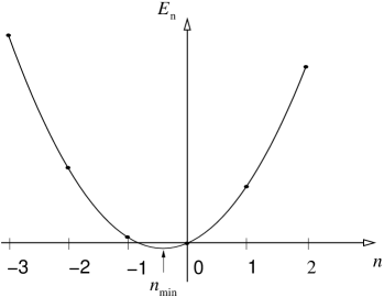
Figure 3: Parabolic spectrum $\epsilon_{n}$ with minimum at $n_{\rm min}=-m\Omega R^{2}/\hbar$ when taken as a function of the continuous parameter $n$.

III.1.2 thermal gas

The ground-state solution $\hat{\Phi}_{1}^{(0)}(x)=\hat{\Phi}_{1,n=0}^{(0)}=\hat{\Phi}_{0}=const.$ means that the atoms do not follow the motion of the trap. This is strictly speaking only possible if the gas is superfluid. In a normal gas collisions with wall roughnesses and between atoms, which are not taken into account here, would accelerate the vapor particles in the initial phase of rotation. Eventually an equilibrium state would be reached where the atoms co-rotate with the trap. This can also be seen from a different argument. In a thermal state with $k_{B}T\gg\hbar\Omega+\hbar^{2}/2mR^{2}$ many states in the spectrum of Fig. 3 will be occupied. As a consequence the thermal gas in the ground state attains an average rotational phase ($x=2\pi R$)

$$\overline{\Delta\phi}=-2\pi\langle n\rangle\to-2\pi\,n_{\rm min}=\frac{2\pi\Omega R^{2}}{\hbar/m}.$$ (31)

This is just the matter-wave Sagnac phase and is in sharp contrast to the case of a Bose-Einstein condensate, where the ground state does not acquire any rotational phase. Since now both, the ground state $|1\rangle$ and the excited state $|2\rangle$ attain the same Sagnac phase shift, the matter-wave contribution to the polarization is exactly cancelled. Thus the extention to thermal gases made in Zimmer and Fleischhauer (2004) is not correct.

The need for a superfluid gas (e.g. BEC) in a ring trap puts restrictions to the achievable interferometer area. Although recently there has been substantial progress in realizing ring traps for BEC Gupta et al. (2005); Arnold et al. (2006), the area achieved is only on the order of 10^-1 cm², which cannot compete with the values reached in fiber-optical gyroscopes.

III.2 Effect of longitudinal confinement

Let us now discuss the case of a longitudinal trapping potential for atoms in state $|1\rangle$, i.e. $V_{1}(x)\neq 0$ in eq. (20). In this case the substitution

$${\hat{\Phi}}_{1}^{(0)}(x)={\hat{\Phi}}_{0}\,f(x)\,{\rm e}^{-{\rm i}m\Omega Rx/\hbar}$$ (32)

leads to the steady-state equation

$$\left(\frac{\hbar^{2}\partial_{x}^{2}}{2m}+\frac{m}{2}\Omega^{2}R^{2}+\epsilon_{1}-V_{1}(x)\right){f}(x)=0.$$ (33)

If one disregards the small centrifugal energy shift proportional to $\Omega^{2}$, this equation is just the stationary Schrödinger equation for a particle in the trap potential $V_{1}$. The solution of this equation is independent of the rotation rate $\Omega$. (The inclusion of the centrifugal term would lead to a higher order contribution to the Sagnac phase, which we are not interested in.) If we substitute (32) into the second equation of (22), one recognizes that all terms containing the rotation rate $\Omega$ vanish exactly:

$$\hat{\Phi}_{2}^{(1)} = -{\rm i}\frac{\hat{\Phi}_{1}^{(0)}(x)}{|\Omega_{c}|^{2}}\left(\eta v_{\rm rec}(\partial_{x}\ln f(x))\Omega_{p}(x)-{\rm i}\frac{\hbar\partial_{x}^{2}}{2m}\Omega_{p}(x)\right)$$ (34)

$$-{\rm i}\frac{\hat{\Phi}_{1}^{(0)}(x)}{|\Omega_{c}|^{2}}\left(\eta v_{\rm rec}-{\rm i}\frac{\hbar}{m}\partial_{x}\ln f(x)\right)\partial_{x}\Omega_{p}(x).$$

Substituting this into the shortened wave equation for $\Omega_{p}$ yields

$$\Bigl{[}c\cos^{2}\theta+\Bigl{(}\eta v_{\rm rec} - {\rm i}\frac{\hbar}{m}\partial_{x}\ln f(x)\Bigr{)}\sin^{2}\theta\Bigr{]}\partial_{x}\Omega_{p}(x)$$

$$-{\rm i}\sin^{2}\theta\frac{\hbar\partial_{x}^{2}}{2m}\Omega_{p}(x) = -{\rm i}k_{p}\Omega R\,\cos^{2}\theta\,\Omega_{p}(x)$$

$$+ \eta v_{\rm rec}\sin^{2}\theta\Bigl{(}\partial_{x}\ln f(x)\Bigr{)}\Omega_{p}(x).$$

Neglecting the term with the second order derivative as well as those containing $\partial_{x}f(x)$, which amounts to assume that $f(x)$ is a slowly-varying ground-state wave function of a sufficiently smooth potential, eq.(III.2) reduces to

$$\partial_{x}\ln\Omega_{p}(x) =-{\rm i}\frac{2\pi\Omega R}{\lambda c}\frac{\cos^{2}\theta}{\cos^{2}\theta+\eta\,v_{\rm rec}\sin^{2}\theta}$$

$$=-{\rm i}\frac{2\pi\Omega R}{\lambda c}\frac{1}{1+\eta\,c/\xi},$$ (36)

It is immediately obvious that only the light part of the Sagnac phase survives. Thus in the EIT hybrid gyroscope a matter-wave contribution to the Sagnac phase only emerges in the absence of a confining potential or if periodic boundary conditions apply as e.g. in a ring trap.

The physical interpretation of this result is straight forward. In the presence of a confining potential the atoms in state $|1\rangle$ are bound to the motion of the confining potential. Hence they acquire a rotational phase shift by following the motion of the trap attached to the rotating frame Hendriks and Nienhuis (1990). Atoms in state $|2\rangle$ acquire the same phase shift since they are in the same frame. Therefore, the polarization attains no Sagnac phase as it is a sesqilinear function of the wave-functions of states $|1\rangle$ and $|2\rangle$. This is in contrast to a superfluid BEC in a ring trap, where the order parameter does not acquire any phase due to the periodic boundary conditions as long as the rotation is sufficiently slow.

IV Quantum limited sensitivity of the slow-light gyroscope

We now want to calculate the sensitivity of the slow-light Sagnac interferometer in the case of periodic boundary conditions, i.e. in the absence of any confining potential in the propagation direction. For simplicity we consider the case $\eta=1$, i. e. perpendicular propagation directions of probe and control field.

To determine the sensitivity we assume that the error in determining the Sagnac phase is entirely given by shot-noise quantum fluctuations. If coherent laser light or Poissonian particle sources are used the shot-noise limit of the phase measurement is given by

$$\Delta\phi_{\rm noise}=\frac{1}{\sqrt{n_{\rm D}}},$$ (37)

where $n_{\rm D}=I_{\rm out}t_{\rm D}$ is the total number of photons or atoms counted at the detector during the measurement time $t_{\rm D}$ Scully and Zubairy (1997). Here $I_{\rm out}$ is the photon or atom flux. The assumption that the quantum noise limit is set by shot-noise is justified by two observations: First of all, it is well known that using nonclassical light or sub-Poissonian particle sources does in general not lead to an improvement of the signal-to-noise ratio in interferometry since at the optimum operation point the amplitude reduction due to losses is typically of order ${\rm e}^{-1}$ and thus quite substantial. These losses tend to quickly destroy the fragile nonclassical and sub-Poissonian properties. Secondly, as has been shown in Scully and Fleischhauer (1992); Fleischhauer et al. (1992), atomic noise contributions in EIT-type interferometer set-ups are small and can be neglected.

In the weak-signal limit discussed in the previous section, the Sagnac phase accumulated is independent of the signal field strength Zimmer and Fleischhauer (2004), hence the signal-to-noise ratio could become arbitrarily large when the input-laser power is increased. In reality the Sagnac phase approaches a maximum value at a certain optimum probe-laser power and decreases for larger intensities. The optimum intensity is reached when the number density of photons in the EIT medium approaches that of the atoms. Thus in order to calculate the maximum sensitivity and to find optimum operation conditions we have to calculate the Sagnac phase to all orders of the signal Rabi frequency $\Omega_{p}$. Since in higher order perturbation the excited state $|3\rangle$ attains a finite population, decay out of the excited state needs to be taken into account. The decay leads to a population redistribution among the states of the $\Lambda$ system, see Fig. 4. It can also lead to loss out of the system. We will disregard the latter process however. Furthermore, we assume that the density of the considered medium is low enough that it is sufficent to describe the system by a set of equations for the single-particle density matrix elements $\rho_{\mu\nu}(x,x^{\prime},t)=\langle{\hat{\Phi}}^{\dagger}_{\nu}(x^{\prime},t){\hat{\Phi}}_{\mu}(x,t)\rangle$. Here $\mu,\nu\in\{1,2,3\}$ denote the internal states. Since the medium polarization is determined by the local density-matrix element $\rho_{12}(x,x,t)$, i.e. $x^{\prime}=x$, we consider only local quantities. For the density matrix elements diagonal in the internal states we find the equations of motion

$$\partial_{t}\rho_{\rm 11}(x,t) =\gamma_{1}\rho_{\rm 22}(x,t)-{\rm i}\,\Omega_{\rm p}^{*}(x,t)\rho_{\rm 21}(x,t)+{\rm i}\,\Omega_{\rm p}(x,t)\rho_{\rm 12}(x,t)+\Omega R\,\partial_{x}\rho_{\rm 11}(x,t),$$ (38)

$$\partial_{t}\rho_{\rm 22}(x,t) =-\gamma_{2}\rho_{\rm 22}(x,t)+{\rm i}\,\Omega_{\rm p}^{*}(x,t)\rho_{\rm 21}(x,t)-{\rm i}\,\Omega_{\rm p}(x,t)\rho_{\rm 12}(x,t)$$

$$+{\rm i}\,\Omega_{\rm c}^{*}(x,t)\rho_{\rm 23}(x,t)-{\rm i}\,\Omega_{\rm c}(x,t)\rho_{\rm 32}(x,t)+(\Omega R+v_{\rm rec})\partial_{x}\rho_{\rm 22}(x,t),$$ (39)

$$\partial_{t}\rho_{\rm 33}(x,t) =\gamma_{3}\rho_{\rm 22}(x,t)-{\rm i}\,\Omega_{\rm c}^{*}(x,t)\rho_{\rm 23}(x,t)+{\rm i}\,\Omega_{\rm c}(x,t)\rho_{\rm 32}(x,t)$$

$$+(\Omega R+v_{\rm rec})\partial_{x}\rho_{\rm 33}(x,t).$$

Likewise we find for the local coherences

$$\partial_{t}\rho_{\rm 12}(x,t) =-({\rm i}(\Delta_{2}+\Omega Rk_{\rm p})+\gamma_{2}/2)\rho_{\rm 12}(x,t)+{\rm i}\,\Omega_{\rm c}^{*}(x,t)\rho_{\rm 13}(x,t)$$

$$-{\rm i}\,\Omega_{\rm p}^{*}(x,t)(\rho_{\rm 22}(x,t)-\rho_{\rm 11}(x,t))+(\Omega R+v_{\rm rec})\partial_{x}\rho_{\rm 12}(x,t)$$

$$+v_{\rm rec}\langle\hat{\Phi}_{\rm 2}^{\dagger}(\partial_{x}\hat{\Phi}_{\rm 1})\rangle\,,$$ (41)

$$\partial_{t}\rho_{\rm 13}(x,t) =-({\rm i}(\Delta_{3}+\Omega Rk_{p})+\gamma_{13})\rho_{\rm 13}(x,t)-{\rm i}\,\Omega_{\rm p}^{*}(x,t)\rho_{\rm 23}(x,t)$$

$$+{\rm i}\,\Omega_{\rm c}(x,t)\rho_{\rm 12}(x,t)+(\Omega R+v_{\rm rec})\partial_{x}\rho_{\rm 13}(x,t)+v_{\rm rec}\langle\hat{\Phi}_{\rm 3}^{\dagger}(\partial_{x}\hat{\Phi}_{\rm 1})\rangle\,,$$ (42)

$$\partial_{t}\rho_{\rm 23}(x,t) ={\rm i}(\Delta_{2}-\Delta_{3})-\gamma_{2}/2)\rho_{\rm 23}(x,t)-{\rm i}\,\Omega_{\rm p}(x,t)\rho_{\rm 13}(x,t)$$

$$-{\rm i}\,\Omega_{\rm c}(x,t)(\rho_{\rm 33}(x,t)-\rho_{\rm 22}(x,t))+(\Omega R+v_{\rm rec})\partial_{x}\rho_{\rm 23}(x,t).$$ (43)

where $\gamma_{2}\equiv\gamma_{1}+\gamma_{3}$. In the following we determine the Sagnac phase shift for arbitrary probe-field Rabi frequency based on the above set of equations and the shortened wave equation. To derive a transparent expression for the rotationally induced phase shift further simplifications are however necessary.

IV.1 Non-local terms

One recognizes from eq. (41) and (42) that the local off-diagonal matrix elements are coupled to non-local quantities of the form $\langle\hat{\Phi}^{\dagger}_{\rm\mu}(x)(\partial_{x}\hat{\Phi}_{\rm\nu}(x))\rangle$. These terms cause the build-up of coherences between different internal states and different positions, which are zero in lowest-order perturbation. We now want to argue that these terms can be neglected. To this end we consider eq. (22) again disregarding second-order derivates and set $V_{3}\equiv\epsilon_{3}\equiv 0$. Hence we have

$$\hat{\Phi}_{2}=\frac{k_{p}\Omega R}{|\Omega_{c}|^{2}}\hat{\Phi}_{1}\Omega_{p}-{\rm i}\frac{\Omega R+v_{\rm rec}}{|\Omega_{c}|^{2}}\partial_{x}(\hat{\Phi}_{1}\Omega_{p}).$$ (44)

Substituting this into the steady-state version of the equation of motion for $\hat{\Phi}_{1}$, eq. (16), remembering that there is no confining potential for atoms in state $|1\rangle$ in the propagation direction, we find

$$\partial_{x}\hat{\Phi}_{1}(x)=-{\rm i}s\frac{\bigl{[}k_{p}\Omega R-{\rm i}(\Omega R+v_{\rm rec})(\partial_{x}\ln\Omega_{p})\bigr{]}}{\Omega R(1+s)+v_{\rm rec}s}\hat{\Phi}_{1}(x),$$ (45)

where $s=|\Omega_{p}|^{2}/|\Omega_{c}|^{2}$ is a saturation parameter. Since the probe field picks up a Sagnac phase shift, we have

$$\partial_{x}\ln\Omega_{p}\sim-{\rm i}\frac{\alpha}{c}k_{p}\Omega R.$$ (46)

With the help of this we finally arrive at

$$\partial_{x}\hat{\Phi}_{1}=-{\rm i}\frac{k_{p}\Omega R}{v_{\rm rec}}\left(1-\alpha\frac{v_{\rm rec}}{c}\right)\hat{\Phi}_{1}+\mathcal{O}\Bigl{(}(\Omega R)^{2}\Bigr{)}.$$ (47)

As a consequence the term $v_{\rm rec}\langle\hat{\Phi}^{\dagger}_{2}\partial_{x}\hat{\Phi}_{1}\rangle$ in eq. (41) is of the order of

$$v_{\rm rec}\langle\Phi^{\dagger}_{2}\partial_{x}\Phi_{1}\rangle\simeq-{\rm i}k_{p}\Omega R\left(1-\alpha\frac{v_{\rm rec}}{c}\right)\rho_{12}$$ (48)

and is thus negligible as compared to $\gamma_{2}\rho_{12}/2$. Using similar arguments one finds that the term $v_{\rm rec}\langle\Phi^{\dagger}_{3}\partial_{x}\Phi_{1}\rangle$ in eq. (42) is of the order of

$$v_{\rm rec}\langle\Phi^{\dagger}_{3}\partial_{x}\Phi_{1}\rangle\simeq-{\rm i}k_{p}\Omega R\left(1-\alpha\frac{v_{\rm rec}}{c}\right)\rho_{13}.$$ (49)

Since ideally the ground-state coherence is long-lived, one has $\gamma_{13}\to 0$. Hence neglecting this term is not as straight forward as for eq.(48). However, adiabatically eliminating the fast decaying optical coherence $\rho_{12}$ in eq. (41) and substituting the resulting expression into the equation of motion of $\rho_{13}$, eq. (42), yields a term proportional to $|\Omega_{c}|^{2}\gamma_{2}\rho_{13}/2$ which is much larger than $k_{p}\Omega R\rho_{13}$. Thus also the term $v_{\rm gr}\langle\hat{\Phi}_{3}^{\dagger}\partial_{x}\hat{\Phi}_{1}\rangle$ can be safely neglected. As a result of this approximation the density matrix equations (38)-(43) are self-contained and local.

Figure 4: $\Lambda$ configuration in which the Rabi frequency $\Omega_{p}$ drives the $1\leftrightarrow 2$-transition and $\Omega_{c}$ the $3\leftrightarrow 2$-transition (solid lines). Radiative decay from the excited level to $|1\rangle$ or to $|3\rangle$ goes as $\gamma_{\rm 1}$ or $\gamma_{\rm 3}$ respectively (dashed lines). The dephasing rate of the $1-3$ coherence is denoted by $\gamma_{13}$.

IV.2 Perturbation theory with respect to characteristic length

In the following we assume one- and two-photon resonance, i.e. $\Delta_{2}=\Delta_{3}=0$, and solve the above system of equations for the coherence of the $|1\rangle\leftrightarrow|2\rangle$-transition in steady state to all orders in $\Omega_{p}$. The density matrix equations (38)-(43) can, neglecting terms proportional to $\Omega R\partial_{x}$, be written in compact form as

$$\dot{\rho}(x,t)=\Bigl{(}{\mathbf{M}}(x)+v_{\rm rec}{\mathbf{D}}\partial_{x}\Bigr{)}\rho(x,t),$$ (50)

where ${\mathbf{M}}$ and ${\mathbf{D}}$ are $9\times 9$ matrices. Even under stationary conditions we are still left with a set of first order linear differential equations with space dependent coefficient. Thus in order to find an analytic solution further approximations are needed. To this end, we make use of the fact that the off-diagonal density matrix elements are only slowly varying in space. Let $L$ and $T$ be their characteristic length and time scales. Normalizing time and space to these units by $\xi=x/L$ and $\tau=t/T$, eq.(50) reads

$$\partial_{\tau}\rho=\left(\tilde{\mathbf{M}}+\frac{v_{\rm rec}T}{L}\tilde{\mathbf{D}}\,\partial_{\xi}\right)\rho$$ (51)

where typical matrix elements of $\tilde{\mathbf{M}}={\mathbf{M}}T$ read as $k_{p}R\Omega T$, with $k_{p}R,|\Omega T|\gg 1$ and those of $\tilde{\mathbf{D}}={\mathbf{D}}T$ are of order unity. Since $v_{\rm rec}T/L$ is typically small compared to unity we can apply a perturbation expansion in this parameter.

In zeroth order we disregard the term containing ${\mathbf{D}}$. Hence in steady state we have to solve ${\mathbf{M}}\rho^{(0)}_{\rm ss}=0$ with the constraint $\sum_{\mu}\rho_{\mu\mu}(x)=n(x)$, which reflects the conservation of probability.

In first order we find

$$\underline{\rho}_{\rm ss}^{(1)}(x)=\Bigl{(}\underline{{\mathbf{1}}}-v_{\rm rec}\underline{{\mathbf{M}}}^{-1}\underline{{\mathbf{D}}}\partial_{x}\Bigr{)}\,\underline{\rho}_{\rm ss}^{(0)}(x).$$ (52)

Here $\underline{\mathbf{M}}$ is a reduced $8\times 8$ matrix obtained from ${\mathbf{M}}$ by incorporating the constraint $\sum_{\mu}\rho_{\mu\mu}(x)=n(x)$ and $\underline{\rho}_{\rm ss}^{(0)}$ is the corresponding zeroth-order density matrix. The explicit expressions of all matrices and vectors can be obtained from (38)-(43) in a straight forward manner. They are however lengthy and will not be given here.

IV.3 Steady state Maxwell-Bloch equation

To obtain the rotationally induced phase shift we expand eq. (52) up to first order in the angular velocity $\Omega$ and use the time-independent Maxwell equation (15) in the rotating frame

$$\Bigl{(}c\partial_{x}-{\rm i}k_{\rm p}\Omega R\Bigr{)}\Omega_{\rm p}(z)=-{\rm i}\,g^{2}N\rho_{\rm 21}^{\rm ss}.$$ (53)

To determine $\rho_{\rm 21}^{\rm ss}$ we furthermore neglected terms ${\mathcal{O}}(\gamma_{\rm 13}^{2})$ and $\gamma_{\rm 13}\Omega_{\rm p}^{n}$ with $n\in{\mathbb{N}}$ since we assume a long-lived coherence between the two lower states $|1\rangle$ and $|3\rangle$. In addition to this we made use of the EIT condition $\Omega_{\rm c}^{2}\gg\gamma_{\rm 13}\gamma_{\rm 1}$ Fleischhauer et al. (2005) and assumed for simplicity $\gamma_{1}=\gamma_{3}=\gamma$.

With these assumptions we arrive at the following expressions for the real and imaginary part of the susceptibility, which determine the dispersion and absorption of the medium

$$\chi^{\,\prime}(\Omega_{\rm p})=\beta^{-1}\,\frac{\displaystyle\Omega\,R}{\displaystyle c}\left(1+g^{2}N\frac{\displaystyle\Omega_{\rm c}^{2}}{\displaystyle(\Omega_{\rm c}^{2}+|\Omega_{\rm p}|^{2})^{2}}\right)$$ (54)

$$\chi^{\,\prime\prime}(\Omega_{\rm p})=-\beta^{-1}\frac{\displaystyle\gamma_{\rm 13}}{\displaystyle k_{p}c}g^{2}N\frac{\displaystyle\Omega_{\rm c}^{2}}{\displaystyle(\Omega_{\rm c}^{2}+|\Omega_{\rm p}|^{2})^{2}}$$ (55)

with

$$\beta(\Omega_{\rm p})=\displaystyle 1+\frac{\displaystyle v_{\rm rec}}{\displaystyle c}g^{2}\,N\frac{\Omega_{\rm c}^{4}}{(\Omega_{\rm c}^{2}+|\Omega_{\rm p}|^{2})^{3}}.$$ (56)

The imaginary part of the complex susceptibility $\chi(\Omega_{\rm p})=\chi^{\,\prime}+{\rm i}\,\chi^{\,\prime\prime}$ can be further simplified. One can easily see that the absorption constant is bounded from above by

$$\kappa=k_{p}\chi^{\prime\prime}\leq\frac{\gamma_{13}}{c}\frac{g^{2}N}{\Omega^{2}_{\rm c}}=\frac{\gamma_{13}}{v_{\rm rec}}\xi^{-1}.$$ (57)

In this limiting case the following equation arises

$$\partial_{z}\ln\Omega_{\rm p}(z)=-\frac{\gamma_{13}}{c}\tan^{2}\theta+{\rm i}\,k_{p}\,\chi^{\,\prime}(\Omega_{\rm p}).$$ (58)

The first term in eq. (58) describes absorption losses due to the nonvanishing decay of the ground-state coherence, the second term the rotationally induced or Sagnac phase. Since the saturation of the absorption for increasing probe-field intensities is not taken into account, the losses are slightly overestimated.

IV.4 Quantum limit of gyroscope sensitivity

Solving the shortened Maxwell equation (58) for the probe field with the all-order susceptibility, eq.(54), we can now determine the minimum detectable rotation rate $\Omega_{\rm min}$ of the slow-light gyroscope. This is done by maximizing the signal-to-noise ratio (SNR) of the interferometer with respect to the system parameters and set it equal to unity. The relative rotational phase shift of two polaritons propagating in opposite directions is given by

$$\Delta\phi_{\rm sig}=\int\!{\rm d}x\,k_{p}\Bigl{[}\chi^{\prime}\bigl{(}\Omega,\Omega_{p}(x)\bigr{)}-\chi^{\prime}\bigl{(}-\Omega,\Omega_{p}(x)\bigr{)}\Bigr{]}.$$ (59)

Using this and eq. (54) we find

$$\Delta\phi_{\rm sig} = \frac{2\pi\Omega R}{\lambda c}\int\!{\rm d}x\,\frac{\xi(x)}{\xi(x)+\frac{1}{(1+s(x))^{3}}}+$$ (60)

$$+\frac{\Omega R}{\hbar/m}\int\!{\rm d}x\,\frac{\frac{1}{(1+s(x))^{2}}}{\xi(x)+\frac{1}{(1+s(x))^{3}}},$$

where $s(x)=|\Omega_{p}(x)|^{2}/\Omega_{c}^{2}$ is the saturation parameter introduced before, and $\xi(x)$, defined in eq. (29), determines the character of the polariton. One recognizes that the matter-wave part of the signal phase - the second line of eq. (60) - decreases for increasing input probe intensity. The light part - first term in eq. (60) - approaches a constant value in this limit. At the same time the shot-noise phase error

$$\Delta\phi_{\rm noise}=\frac{1}{\sqrt{n_{D}}}$$ (61)

is inversely proportional to $|\Omega_{p}(0)|\,\exp\left(-\kappa L_{M}\right)$, where $L_{M}$ is the length of the medium and the probe-field’s source is located at $x=0$. As a consequence of the different dependence of the signal and noise terms on the probe field strength, the signal-to-noise ratio SNR $=\Delta\phi_{\rm sig}/\Delta\phi_{\rm noise}$ has the qualitative behavior shown in Fig. 5.

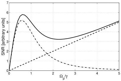
Figure 5: Schematic dependence of SNR on input probe-field Rabi frequency. The dash-dotted line indicates the contribution of the matter-wave term, the dashed line that of the light term. The solid line is the sum of both contributions.

For very large laser fields the SNR becomes arbitrarily large, as the light contribution to the Sagnac phase becomes intensity independent and the shot-noise level decreases steadily. For small probe intensities the SNR has a local maximum due to the saturation of the matter-wave phase shift. As the matter-wave contribution to the Sagnac phase is orders of magnitude larger than the light contribution, extremely large input intensities would be required to exceed the sensitivity at the first local maximum. (Note that Fig. 5 is not drawn to scale.) We thus consider only this first maximum when determining the quantum-limited sensitivity of the slow-light gyroscope.

Although it is rather straight forward to calculate numerically, on the basis of the above given equations the minimum detectable rotational phase shift, we are interested here in an analytic estimate. For this we make some simplifying assumptions: First of all we consider the propagation of polaritons through a homogeneous medium. We furthermore ignore the space dependence of the functions $\xi(x)$ and $s(x)$ in the expression (60) for the signal phase, which amounts to replacing $|\Omega_{p}(x)|$ by its input value $|\Omega_{p}(0)|\equiv|\Omega_{p}|$. As will be seen this only slightly overestimates the saturation of the signal at the optimum operation point. We also ignore the saturation of the probe field absorption, which again merely slightly overestimates the probe field losses at the operation point. Finally we only consider the dominant matter-wave contribution to the signal phase. Thus we have

$$\Delta\phi_{\rm sig}=\frac{\Omega RL}{\hbar/m}\frac{(1+s)}{\xi(1+s)^{3}+1}.$$ (62)

In order to estimate the signal-to-noise ratio SNR $=\Delta\phi_{\rm sig}/\Delta\phi_{\rm noise}$ we now express the the shot-noise expression (61) in terms of the parameters $\xi$ and $s$. The number of probe photons at the detector can be written in terms of the probe-field Rabi frequency at the source via

$$n_{\rm D}=\frac{P_{\rm D}t}{\hbar\omega_{\rm p}}=\frac{2\,\epsilon_{0}\,F\,c}{\hbar\omega_{p}}\left(\frac{\hbar\,\Omega_{p}(0)}{|{\mathbf{d}}_{p}|}\right)^{2}\,t\,e^{-2\kappa L_{M}},$$ (63)

where $F$ is the cross-section of the signal beam, $t$ the detection time interval, and $\kappa=\gamma_{13}/(v_{\rm rec}\xi)$ the absorption coefficient introduced before. The radiative decay rate $\gamma=\gamma_{1}$ and the dipole matrix element $|{\mathbf{d}}_{p}|$ contained in the Rabi frequency $\Omega_{p}(0)$ are related through

$$\gamma=\frac{1}{4\,\pi\,\epsilon_{0}}\left(\frac{4}{3}\frac{|{\mathbf{d}}_{p}|^{2}\,\omega^{3}_{p}}{\hbar\,c^{3}}\right),$$ (64)

i. e. according to the Einstein A-coefficient Mandel and Wolf (1995). After a straight forward calculation we find

$$n_{\rm D}=F\,\varrho\,v_{\rm rec}\,t\,\xi\,s\,{\rm e}^{-2\,a/\xi}$$ (65)

where $\varrho$ is the density of atoms in the EIT medium, and

$$a\equiv\frac{\gamma_{13}L_{M}}{v_{\rm rec}}$$ (66)

characterizes the absorption due to a finite lifetime of the ground-state coherence. Since typical values of $\gamma_{13}$ are in the kHz regime and $v_{\rm rec}\sim 1$ cm/s, $a$ is typically large compared to unity for $L_{M}\gg 10^{-3}$ cm. With the above expressions we find for the signal-to-noise ratio

SNR $$= \frac{\Omega\,A}{\hbar/m}\Bigl{(}F\,\varrho\,v_{\rm rec}\,t\Bigr{)}^{1/2}$$ (67)

$$\times\frac{\xi^{1/2}s^{1/2}(1+s)}{\xi(1+s)^{3}+1}\,e^{-a/\xi}.$$

The first two factors in eq. (67) are the signal-to-noise ratio of a pure matter-wave gyroscope with interferometer area $A=RL_{M}$ and a flux of atoms corresponding to a density of atoms $\varrho$ passing through an area $F$ with recoil velocity $v_{\rm rec}$. In conventional atomic interferometers based on cold or ultra-cold atoms the flux that contributes to the interference signal of the device is rather low. It is on the order of $10^{8}$ atoms/s in comparison with $10^{16}$ photons/s in a conventional fiber-optics gyroscope Kasevich (2002). However, in the case studied here, the flux can be at least two orders of magnitude higher than in an atom interferometer.

The second factor can be modified by optimizing the probe field strength ($s$) and the group velocity in the medium ($\xi$). In Fig. 6 we have plotted the optimum values of $s$ and $\xi$ derived by maximizing the signal-to-noise ratio for different values of the loss parameter $a$.

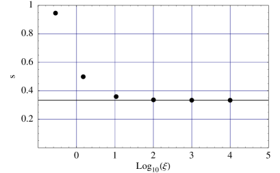
Figure 6: Optimum values of $s=|\Omega_{p}(0)|^{2}/\Omega^{2}_{c}$ and $\xi=v_{\rm gr}/v_{\rm rec}-1$ for different values of the loss parameter $a=\gamma_{13}L_{M}/v_{\rm rec}$ ($=0.05,0.5,5,50,500,5000$). For large values of $a$ the optimum values are $s_{\rm opt}=1/3$ and $\xi_{\rm opt}=2a$. For small values of $a$ there is only a small deviation in the optimum parameters.

One finds that in the typical parameter regime $a\gg 1$ the maximum SNR is attained for

$$s_{\rm opt}=\frac{1}{3},\quad\textrm{and}\quad\xi_{\rm opt}=2a.$$ (68)

Note that this approximation is still quite good even when $a=1$. The optimum group velocity is given by

$$v_{\rm gr}^{\rm opt}=2\gamma_{13}L+v_{\rm rec}\approx 2\gamma_{13}L_{M},$$ (69)

i.e. a maximum SNR is achieved if the velocity is chosen such that during the propagation over the entire medium length $L_{M}$, a fraction of $1/\sqrt{e}$ of the initial polariton gets absorbed. Setting SNR $=1$ we eventually obtain the minimum detectable rotation rate

$$\Omega_{\rm min}=\frac{\hbar/m}{A}\frac{1}{\bigl{(}F\,\varrho\,v_{\rm rec}\,t\bigr{)}^{1/2}}\,f\,\sqrt{a}$$ (70)

where $f\approx 7.2$ is a numerical prefactor resulting from the optimization of the term in the second line of eq.(67). Apart from the term $\sqrt{a}$ and the unimportant numerical prefactor $f$, the minimum detectable rotation rate corresponds to that of a matter-wave interferometer with atoms propagating at recoil velocity. The densities achievable in the present set-ups, e.g. if we consider BECs in ring trap configurations, are however much larger than those in typical atomic beams.

To be more precise we give an estimate for the minimum detectable rotation rate of the slow-light gyroscope achievable with current technology. To this end we consider two state-of-the-art circular waveguides for Bose-Einstein condensates Gupta et al. (2005); Arnold et al. (2006). Furthermore, we assume that the atomic density of the BECs is $\rho=10^{14}$ cm^-3 with a cross-section (smaller circle of the toroidal BEC) of $F\approx 10^{-2}$ cm². In case of the work of S. Gupta et al. Gupta et al. (2005) the diameter of the larger circle of the toroidal waveguide is $d_{\rm Gupta}\approx 3$ mm and in the case of A. S. Arnold et al. Arnold et al. (2006) it is $d_{\rm Arnold}\approx 96$ mm. Hence, we find in the first case the minimum detectable rotation rate to be $\Omega_{\rm min}^{\rm Gupta}\approx 1.4\times 10^{-9}$ s^-1 Hz^-1/2 and in the latter case $\Omega_{\rm min}^{\rm Arnold}\approx 1.4\times 10^{-12}$ s^-1 Hz^-1/2. These values should be compared to the state of the art which for optical gyroscopes is $2\times 10^{-10}$ rad s^-1 Hz^-1/2 Stedman et al. (2003) and for matter-wave gyroscopes $6\times 10^{-10}$ rad s^-1 Hz^-1/2 Gustavson et al. (2000).

V Conclusion

We have analyzed in detail a novel type of light-matter-wave hybrid Sagnac interferometer based on ultra-slow light in media with electromagnetic induced transparency (EIT) proposed by us in Zimmer and Fleischhauer (2004). In particular the influence of confining potentials was investigated and the shot-noise limited sensitivity and the minimum detectable rotation rate determined. By combining features of light and matter-wave devices the hybrid interferometer yields a minimum detectable rotation rate which is potentially better than the currect state of the art by up to two orders of magnitude. We have shown that as opposed to claims in earlier proposals for slow-light gyroscopes Leonhardt and Piwnicki (2000), it is not sufficient to utilize only the dispersive properties of EIT-media to achieve an enhancement of the rotation sensitivity. It is rather necessary to employ simultaneously coherence and momentum transfer in the associated Raman transition. Moreover we have shown that the medium has to be prepared in a state in which it does not acquire any rotational phase shift. This can be achieved for example by using a superfluid BEC in a ring trap as EIT medium. The requirement for periodic boundary conditions reduces the potential of the hybrid interferometer idea as compared to the statements in Zimmer and Fleischhauer (2004) as it is not possible to build large area interferometers under this condition with current technology. However, the potential large flux of the proposed slow-light interferometer leads to a substantial reduction of the shot noise as compared to state-of-the-art matter-wave gyroscopes and thus leads nevertheless to a substantial sensitivity enhancement.

References

- Sagnac (1913) M. G. Sagnac, Comp. Rend. Acad. Sci. 157, 708 (1913), Paris.
- Post (1967) E. J. Post, Rev. Mod. Phys. 39, 475 (1967).
- Chow et al. (1985) W. W. Chow, J. Gea-Banacloche, L. M. Pedrotti, V. E. Sanders, W. Schleich, and M. O. Scully, Rev. Mod. Phys. 57, 61 (1985).
- Stedman (1997) G. E. Stedman, Rep. Prog. Phys. 60, 615 (1997).
- Bongs and Sengstock (2004) K. Bongs and K. Sengstock, Rep. Prog. Phys. 67, 907 (2004).
- Scully and Zubairy (1997) M. O. Scully and M. S. Zubairy, Quantum Optics (Cambridge University Press, Cambridge, 1997).
- Page (1975) L. A. Page, Phys. Rev. Lett. 35, 543 (1975).
- Gustavson et al. (1997) T. L. Gustavson, P. Bouyer, and M. A. Kasevich, Phys. Rev. Lett. 78, 2046 (1997).
- McGuirk et al. (2000) J. M. McGuirk, M. J. Snadden, and M. A. Kasevich, Phys. Rev. Lett.
- Culshaw (2006) B. Culshaw, Measurement Science & Technology
- Kasevich (2002) M. A. Kasevich, Science 298, 1363 (2002).
- Orzel et al. (2001) C. Orzel, A. K. Tuchman, M. L. Fenselau, M. Yasuda, and M. A. Kasevich, Science 291, 2386 (2001).
- Chikkatur et al. (2002) A. P. Chikkatur, Y. Shin, A. E. Leanhardt, D. Kielpinski, E. Tsikata, T. L. Gustavson, D. E. Pritchard, and W. Ketterle, Science 296, 2193 (2002).
- Zimmer and Fleischhauer (2004) F. Zimmer and M. Fleischhauer, Phys. Rev. Lett. 92,
- Fleischhauer et al. (2005) M. Fleischhauer, A. Imamoğlu, and J. P. Marangos, Rev. Mod. Phys. 77, 633 (pages 41) (2005).
- Fleischhauer and Lukin (2000) M. Fleischhauer and M. D. Lukin, Phys. Rev. Lett. 84, 5094 (2000).
- Hendriks and Nienhuis (1990) B. H. W. Hendriks and G. Nienhuis, Quantum Optics: Journal of the European Optical Society Part B 2, 13 (1990).
- Gupta et al. (2005) S. Gupta, K. W. Murch, K. L. Moore, T. P. Purdy, and D. M. Stamper-Kurn, Phys. Rev. Lett. 95, 143201 (pages 4) (2005).
- Arnold et al. (2006) A. S. Arnold, C. S. Garvie, and E. Riis, Phys. Rev. A (Atomic, Molecular, and Optical Physics) 73, 041606 (pages 4) (2006).
- Dufour and Prunier (1937) A. Dufour and F. Prunier, Comp. Rend. Acad. Sci. 204, 1322 (1937).
- Hau et al. (1999) L. V. Hau, S. E. Harris, Z. Dutton, and C. H. Behroozi, Nature 397, 594 (1999).
- Budker et al. (1999) D. Budker, D. F. Kimball, S. M. Rochester, and V. V. Yashchuk, Phys. Rev. Lett.
- Kash et al. (1999) M. M. Kash, V. A. Sautenkov, A. S. Zibrov, L. Hollberg, G. R. Welch, M. D. Lukin, Y. Rostovtsev, E. S. Fry, and M. O. Scully, Phys. Rev. Lett. 82, 5229 (1999).
- Matsko et al. (2001) A. B. Matsko, O. Kocharovskaya, Y. Rostovtsev, G. R. Welch, A. S. Zibrov, and M. O. Scully, Adv. In Atomic, Molecular, Opt. Physics, Vol 46 46, 191 (2001).
- Cohen-Tannoudji et al. (1997) C. Cohen-Tannoudji, J. Dupont-Roc, and G. Grynberg, Photons and atoms: Introduction to Quantum Electrodynamics (John Wiley & Sons, Inc., 1997).
- Scully and Fleischhauer (1992) M. O. Scully and M. Fleischhauer, Phys. Rev. Lett. 69, 1360 (1992).
- Fleischhauer et al. (1992) M. Fleischhauer, C. H. Keitel, M. O. Scully, C. Su, B. T. Ulrich, and S. Y. Zhu, Phys. Rev. A 46, 1468 (1992).
- Mandel and Wolf (1995) L. Mandel and E. Wolf, Optical coherence and quantum optics (Cambridge University Press, Cambridge, 1995).
- Stedman et al. (2003) G. E. Stedman, K. U. Schreiber, and H. R. Bilger, Classical Quantum Gravity 20, 2527 (2003).
- Gustavson et al. (2000) T. L. Gustavson, A. Landragin, and M. A. Kasevich, Classical Quantum Gravity 17, 2385 (2000).
- Leonhardt and Piwnicki (2000) U. Leonhardt and P. Piwnicki, Phys. Rev. A 62, 055801 (2000).