We discuss a mechanism for generating a maximum entangled state (GHZ) in a coupled quantum dots system, based on analytical techniques. The reliable generation of such states is crucial for implementing solid-state based quantum information schemes. The signature originates from a remarkably weak field pulse or a far off-resonance effects which could be implemented using technology that is currently being developed. The results are illustrated with an application to a specific wide-gap semiconductor quantum dots system, like Zinc Selenide (ZnSe) based quantum dots.

PACS03.67.-a; 32.80.Pj; 42.50.Ct; 42.65.Yj; 03.75.-b

1 Introduction

Excitons (electron-hole bound states) within quantum dots (QDs) have attracted much interest in the field of quantum computation and have formed the basis of several proposals for quantum logic gates [1]. The energy shift due to the exciton-exciton dipole interaction between multi-quantum dots gives rise to diagonal terms in the interaction Hamiltonian, and hence it has been proposed that quantum logic may be performed via ultra-fast laser pulses [2]. However, excitons within adjacent quantum dots are also able to interact through their resonant (Förster) energy transfer, some evidence for which has been obtained experimentally [3]. Because the quantum dot has discrete energy levels, much like an atom, the energy levels can be controlled by changing the size and shape of the quantum dot, and the depth of the potential. Like in atoms, the energy levels of small quantum dots can be probed by optical spectroscopy techniques. In contrast to atoms it is relatively easy to connect quantum dots by tunnel barriers to conducting leads, which allows the application of the techniques of tunneling spectroscopy for their investigation.

Many properties of such systems can be investigated by transport, if the dots are fabricated between contacts acting as source and drain for electrons which can enter or leave the dot [4, 5]. Creating entangled states is the first step toward studying any effects related to entanglement. Semiconductor quantum dots have their own advantages as a candidate of the basic building blocks of solid-state-based quantum logic devices [6, 7, 8], due to the existence of an industrial base for semiconductor processing and due to the ease of integration with existing devices. The experimental realization of optically induced entanglement of excitons in a single quantum dot [9] and theoretical study on coupled quantum dots [10] were reported most recently. In those investigations a classical laser field is applied to create the electron-hole pair in the dot(s).

The issue we have in mind has to do with the exact solution of the system, taking into account the dependence on the relevant magnitudes such as the field strength, inter-dot process hoping rate and the detuning. This is most conveniently accomplished in a quantum formalism in terms of the Schrödinger equation. Related treatments based on either adiabatic elimination [4], discussing entangled state generation conditions, or the coupled equations without the detuning dependence, have been presented in the literature [6]. What we have studied and present below is essentially the most general case of the complete system equations. To be more precise, with this approach we could create maximum entangled states without using the approximation methods adapted in previous studies.

The outline of this paper is arranged as follows: in section 2, we give notations and definitions of the model followed by a rigorous analytical approach for obtaining exact-time dependent expressions for the probability amplitudes. Section 3 is devoted to consider the maximum entangled state generation. By a numerical computation, we examine the influence of different parameters on the evolution of the probability density of finding the maximum entangled state. Finally, our conclusion will be presented in section 4.

2 Model

We characterize the electron and hole states within a quantum dots model, as well as accounting for the binding energy due to electron-hole coupling within a dot when estimating the ground state exciton energy. To begin with, we consider a system with $3$ identical quantum dots that are coupled by the Förster process [11]. This process originates from the Coulomb interaction whereby an exciton can hop between the dots [12]. The Coulomb exchange interaction in QDs gives rise to a non-radiative resonant energy transfer (i.e. Förster process) which corresponds to the exchange of a virtual photon, thereby destroying an exciton in a dot and then re-creating it in a close by dot (for a detailed discussion of how to exploit the Förster interaction see e.g. [10, 13]). The present study is motivated by recent experimental results which demonstrated the optical detection of an NMR signal in single QDs [14]. Hence the underlying nuclear spins in the QDs can indeed be controlled with optical techniques, via the electron-nucleus coupling. Also, few electron dots can be prepared experimentally [15] and their magic number transitions could be measured as a function of magnetic field.

Keeping in mind the fact that all constant energy terms may be ignored, the total Hamiltonian governs the time evolution of single excitons within the individual quantum-dot systems with its interdot Förster hopping and the interaction of the system with the laser field, in an appropriate rotating frame [16], is given by

$$\hat{H}=\hat{H}_{0}+\hat{H}_{F}+\hat{H}_{I},$$ (1)

where, $\hat{H}_{0}$ is the single-exciton Hamiltonian, $\hat{H}_{F}$ is the interdot Förster interaction and $\hat{H}_{I}$ is the coupling of the carrier system with a classical laser field, which can be written as

$$\hat{H}_{0} = \frac{\varepsilon}{2}\sum\limits_{j=1}^{3}\left(\widehat{e}_{j}^{\dagger}\widehat{e}_{j}-\widehat{\psi}_{j}\widehat{\psi}_{j}^{\dagger}\right),$$

$$\hat{H}_{F} = \frac{\hbar\eta}{2}\sum\limits_{j=1}^{3}\sum\limits_{k=1}^{3}\left(\widehat{e}_{j}^{\dagger}\widehat{\psi}_{k}\widehat{e}_{k}\widehat{\psi}_{j}^{\dagger}+\widehat{\psi}_{j}\widehat{e}_{k}^{\dagger}\widehat{\psi}_{k}^{\dagger}\widehat{e}_{j}\right),$$

$$\hat{H}_{I} = \frac{\hbar}{2}\sum\limits_{j=1}^{3}\left(\Omega\exp\left[-i\omega t+i\phi\right]\widehat{e}_{j}^{\dagger}\widehat{\psi}_{j}^{\dagger}+\Omega^{\ast}\exp\left[i\omega t-i\phi\right]\widehat{\psi}_{j}\widehat{e}_{j}\right)$$ (2)

where $\Omega$ represents the Rabi frequency which characterizes the laser-quantum dot coupling and $\hbar\Omega=\mu E$, where $\mu$ is the coupling strength. We denote by $E$, $\phi$ the laser pulse electric field amplitude and phase, respectively. The parameter $\omega$ discribes the angular frequency of the laser field. The operator $\widehat{e}_{j}(\widehat{\psi}_{j})$ is the electron (hole) annihilation operator and $\widehat{e}_{j}^{\dagger}(\widehat{\psi}_{j}^{\dagger})$ is the electron (hole) creation operator in the $j^{\underline{th}}$ quantum dot. The parameter $\varepsilon$ describes the band gap energy of the quantum dot and $\eta$ is the inter-dot process hoping rate.

For a coupled three-quantum-dot system, we consider the $J=3/2$-subspace as the only one optically active (the other $J=1/2$ subspace remains optically dark). We work in the basis set $|J=3/2,M\rangle,\{|0\rangle=|3/2,-3/2\rangle,|1\rangle=|3/2,-1/2\rangle,|2\rangle=|3/2,1/2\rangle,|3\rangle=|3/2,3/2\rangle\}$, where $|0\rangle$ is the vacuum state, $|1\rangle$ is the single-exciton state, $|2\rangle$ is the biexciton state and $|3\rangle$ is the triexciton state. More specifically, applying the rotating wave approximation and a unitary transformation, the resulting Hamiltonian may be written as

$$H = \frac{3}{2}\left(\eta-\Delta\right)\widehat{S}_{11}+\Omega^{\ast}\sqrt{3}e^{-i\phi}\widehat{S}_{12}+\Omega\sqrt{3}e^{i\phi}\widehat{S}_{21}+\frac{1}{2}\left(7\eta-\Delta\right)\widehat{S}_{22}+2\Omega^{\ast}e^{-i\phi}\widehat{S}_{23}$$ (3)

$$+2\Omega e^{i\phi}\widehat{S}_{32}+\frac{1}{2}\left(7\eta+\Delta\right)\widehat{S}_{33}+\Omega^{\ast}\sqrt{3}e^{-i\phi}\widehat{S}_{34}+\Omega\sqrt{3}e^{i\phi}\widehat{S}_{43}+\frac{3}{2}\left(\eta+\Delta\right)\widehat{S}_{44},$$

where $\widehat{S}_{ij}=|i+1\rangle\langle|j+1|$ are related to the above states $|0\rangle,$ $|1\rangle,$ $|2\rangle$ and $|3\rangle.$ We denote by $\Delta$ the detuning of the laser pulse from exact resonance ($\hbar\Delta=\varepsilon-\hbar\omega)$. We consider the situation of a laser pulse with central frequency $\omega$ given by $\xi(t)=\Omega e^{-i\omega t}.$ From a practical point of view, parameters $\Omega$ and $\omega$ are adjustable in the experiment to give control over the system of QDs.

We devote the following discussion to find an explicit expression for the wave function in Schrödinger picture. We use an analytic approach that seeks to reduce the coupled differential equations (probability amplitudes) to a solvable linear equation in order to study in detail the related phenomena. To reach our goal we assume that the wave function of the complete system may be expanded in terms of the eigenstates, namely

$$\left|\Psi(t)\right\rangle=B_{0}(t)\left|0\right\rangle+B_{1}(t)\left|1\right\rangle+B_{2}(t)\left|2\right\rangle+B_{3}(t)\left|3\right\rangle.$$ (4)

The time dependence of the amplitudes in equation (4) is governed by the Schrödinger equation with the Hamiltonian given by equation (3). In order to find the probability amplitudes $B_{i}(t)$, one may introduce the function [17]

$$G(t)=B_{0}(t)+xB_{1}(t)+yB_{2}(t)+zB_{3}(t),$$ (5)

which leads to the following equation

$$i\frac{dG(t)}{dt}=\beta\left(B_{0}(t)+\frac{\gamma_{1}}{\beta}B_{1}(t)+\frac{\gamma_{2}}{\beta}B_{2}(t)+\frac{\gamma_{3}}{\beta}B_{3}(t)\right).$$ (6)

where $\beta=\xi_{00}+x\xi_{10},$ $\gamma_{1}=\xi_{01}+x\xi_{11}+y\xi_{21},{\ \ }\gamma_{2}=x\xi_{12}+y\xi_{22}+z\xi_{32},$ $\gamma_{3}=y\xi_{23}+z\xi_{33},$ and $\xi_{jk}=\left\langle j\right|\hat{H}\left|k\right\rangle.$ In this case and using equations (3) and (4), we have $\xi_{00}=1.5(\eta-\Delta),\xi_{01}=\left(\xi_{10}\right)^{\ast}$ $=\sqrt{3}\Omega\exp(i\phi),$ $\xi_{11}=0.5(7\eta-\Delta),$ $\xi_{12}=\left(\xi_{21}\right)^{\ast}$ $=2\Omega\exp(-i\phi),$ $\xi_{22}=0.5(7\eta+\Delta),$ $\xi_{23}=\left(\xi_{32}\right)^{\ast}$ $=\sqrt{3}\Omega\exp(-i\phi),$ $\xi_{33}=1.5(\eta+\Delta)$ and $\xi_{ij}=0$ otherwise. Now let us seek a solution of $G(t)$ such that $\dot{G}(t)=-i\mu G(t)$. This holds if and only if $\mu=\beta,x=\gamma_{1}/\beta,$ $\ y=\gamma_{2}/\beta$ and $\ z=\gamma_{3}/\beta.$ Therefore, after some minor algebraic calculations, the general solution can be written as

$$B_{j-1}(t)=\exp\left(-i\xi_{11}t\right)\sum\limits_{k=1}^{4}\lambda_{jk}\exp\left(-i\xi_{21}\mu_{k}t\right),{\ \ \ \ }j=1,2,3,4$$ (7)

where

$$\mu_{1,2}=-\frac{\Re_{1}}{4}-\Upsilon_{1}\pm\left(\Upsilon_{2}-\frac{m_{4}}{m_{2}}\right)^{\frac{1}{2}},{\ \ \ \ \ }\mu_{3,4}=-\frac{\Re_{1}}{4}+\Upsilon_{1}\pm\left(\Upsilon_{2}+\frac{m_{4}}{m_{2}}\right)^{\frac{1}{2}},$$ (8)

and $\Upsilon_{1}=\frac{1}{2}\sqrt{\Re_{1}^{2}/4-2\Re_{2}/3+m_{2}/(3m_{1})+m_{1}/(3\sqrt[3]{2})},$ $\Upsilon_{2}=\Re_{1}^{2}/2-4\Re_{2}/3-m_{3}/(3m_{1})-m_{1}/(3\sqrt[3]{2}),$ $m_{1}=\left(m_{0}+\sqrt{-2m_{3}^{2}+m_{0}^{2}}\right)^{1/3},$ $m_{0}=2\Re_{2}^{2}-9\Re_{1}\Re_{2}\Re_{3}+27\Re_{3}^{2}+27\Re_{1}^{2}\Re_{4}-72\Re_{2}\Re_{4},$ $m_{2}=\sqrt[3]{2}\left(\Re_{2}^{2}-3\Re_{1}\Re_{3}+12\Re_{4}\right),$ $m_{3}=4(\Re_{1}^{2}/4-2\Re_{2}/3$ $+m_{3}/(3m_{1})+m_{1}/(3\sqrt[3]{2})),$ $m_{4}=-\Re_{1}^{3}+4\Re_{1}\Re_{2}-8\Re_{3}.$ The parameters $\Re_{i},(i=1,2,3,4)$ are the coefficients of the fourth order equation for $x$ and $\lambda_{ij}=O_{ij}^{-1}G_{j}(0)$.

As a specific dynamical example, we discuss a frequently encountered phenomena of particular interest in which we discuss the generation of maximum entangled GHZ states in the present system.

3 Greenberger–Horne–Zeilinger (GHZ)

There is a class of genuine tripartite entanglement, that is the Greenberger–Horne–Zeilinger (GHZ) state [18, 19] which is given as

$$|GHZ\rangle_{\tau}=\left(\frac{1}{\sqrt{2}}|000\rangle+\frac{\exp(i\tau)}{\sqrt{2}}|111\rangle\right),$$ (9)

for arbitrary values of $\tau$. Starting with a zero-exciton state as an initial state, the probability density $\wp(GHZ)$ of finding the entangled $|GHZ\rangle_{\tau}$ state between vacuum and triexciton states can be calculated in the following form

$$\wp(GHZ) = \left|{}_{\tau}\left\langle GHZ|\Psi(t)\right\rangle\right|^{2}$$ (10)

$$= \frac{1}{2}\left|B_{0}(t)+B_{3}(t)\right|^{2},$$

where $B_{0}(t)$ and $B_{3}(t)$ are given by equation (7).

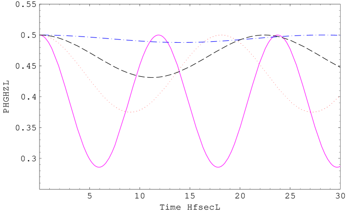
Figure 1: Generation of the GHZ state $\frac{1}{\sqrt{2}}|000\rangle+\frac{\exp(i\tau)}{\sqrt{2}}|111\rangle$. The parameters are $\eta=0.1,$ $\Delta=0,\phi=0$ and for different values of the laser-quantum dot coupling $\Omega=0.1$ $fs^{-1}$ (solid curve), $\Omega=0.05$ $fs^{-1}$ (dotted curve), $\Omega=0.03$ $fs^{-1}$ (dashed curve), and $\Omega=0.01$ $fs^{-1}$ (dotted-dashed curve).

Here we present the results of numerical calculations for a specific wide-gap semiconductor quantum dots system, like Zinc Selenide (ZnSe) based quantum dots, where femtosecond spectroscopy is currently available for these systems [20]. For these materials, the band gap $\epsilon=2.8$ $eV$, which implies a resonant optical frequency $\omega=4.3\times 10^{15}s^{-1}$.

Specifically, we consider the probability density $\wp(GHZ)$ as a function of the scaled time and different values of the laser-quantum dot coupling in figure 1 and different values of the detuning parameter in figure 2. When we consider the parameter $\Omega=0.1$ $fs^{-1},$ we see that the probability density shows periodic oscillations between $2.6$ and $0.51$ (see figure 1). Once the laser-quantum dot coupling is decreased, the amplitude of the oscillations becomes smaller and smaller. Further decreasing of this parameter, we obtain a maximally entangled GHZ state in the system of the three coupled quantum dots i.e $\wp(GHZ)\approx 0.5.$ Also, from figure 1, we see that the selective pulses used to create such maximally entangled GHZ states in the present system is $\pi/2$. The generation of the GHZ state $|GHZ\rangle_{\tau}$ requires a time $1.3\times 10^{-14}$ sec and explore several different ranges for the time pulses required in the generation of such GHZ states.

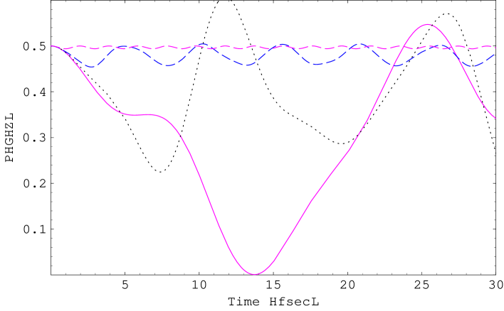
Figure 2: Generation of the GHZ state $\frac{1}{\sqrt{2}}|000\rangle+\frac{\exp(i\tau)}{\sqrt{2}}|111\rangle$. The parameters are $\eta=0.1,$ $\Omega=0.05$ $fs^{-1},\phi=0$ and for different values of the detuning parameter, where $\Delta=0.1\eta$ (solid curve), $\Delta=0.3\eta$ (dotted curve), $\Delta=1.0\eta$ (dashed curve), and $\Delta=3.0\eta$ (dotted-dashed curve).

However, interestingly, this does not mean that there is no other effect due to other parameters of the system in this case. As we show next, there is an effect due to far off-resonance interaction, even though reversing the sign or changing the values of the parameter $\tau$ has no effect. The effect of the detuning parameter on the probability density may be examined by considering the far off-resonance interaction, namely, $\Delta>0.$ Although, we have found that it is not difficult to find maximum entangled state using weak field limit (see figure 1), part of the motivation for this paper grew out of an effort to obtain maximum entangled state using our analytical solution, based on effects of the detuning parameter. This is shown in figure 2, where we plot the probability density $\wp(GHZ)$ as a function of the scaled time for different values of the detuning parameter. All the parameters are identical to those used in figure 1, except for the detuning parameter. As we show, the maximum entangled GHZ state is obtained when the detuning parameter is increased enough  even in the presence of strong field limit (see figure 2). Therefore, the same maximum entangled GHZ state is formed periodically. By choosing a suitable time interval and large detuning, one can effectively obtain $\wp(GHZ)\approx 0.5.$ Now the difference between the effects of the two cases is obvious. Then, the most reliable way to obtain maximum entangled GHZ state is the consideration of the weak field limit or far off-resonant interaction. In the above figures, we have shown how maximally entangled GHZ states can be generated using the optically driven resonant transfer of excitons between quantum dots.  Based on such sensitivity and some other evidence, we suspect that the analytical results presented here, could be attained for a larger number of particles.

4 Conclusion

In summary, an analytical solution for single excitons within three individual ZeSe quantum dots and their interdot hopping in the presence of the Förster interaction has been developed and discussed. Such analytical solutions provide useful physical insight, which together with numerical treatments are used to generate maximum entangled GHZ states. More explicitly, in the exciton system, the large values of the detuning help in generating maximum entangled states.  Nevertheless, the calculations indicate that the maximum entangled states can still exist, even for the resonant case, when the electron and hole are driven by a suitable laser field (weak field limit). This study reveals that the three coupled quantum dots can be used for generating a maximum entangled states, such as GHZ. Paramount importance is acquiring the maximum entangled states due to an ensemble of three quantum dots as it is becoming ubiquitous to different fields of application as quantum computation, quantum information processing and other related fields.

Acknowledgments:

We are indebted to E. Paspalakis, M. Salman and S. S. Hassan for valuable discussions which led to the investigation above.

References

- [1] A. Nazir, B. Lovett, S. Barrett, J. H. Reina, A. Briggs, ”Anticrossings in Förster coupled quantum dots” Phys. Rev. B 71, 045334-045346 (2005)
- [2] T. Brandes, ”Coherent and collective quantum optical effects in mesoscopic systems” Phys. Rep. 408, 315–474 (2005)
- [3] A. J. Berglund, A. C. Doherty, and H. Mabuchi, ”Photon Statistics and Dynamics of Fluorescence Resonance Energy Transfer” Phys. Rev. Lett. 89, 068101-068105 (2002).
- [4] E. Paspalakis and A. F. Terzis, ”Creation of entangled states of excitons in coupled quantum dots” Phys. Lett. A 350, 396-399 (2006)
- [5] E. Paspalakis and M. Abdel-Aty, ”A rigorous analytical approach to an optically driven quantum dots system” Submitted (2006).
- [6] D. Loss and D. P. DiVincenzo, ”Quantum computation with quantum dots” Phys. Rev. A 57, 120-126 (1998).
- [7] R. M. Stevenson, R. J. Young, P. See, D. G. Gevaux, K. Cooper, P. Atkinson, I. Farrer, D. A. Ritchie and A. J. Shields, ”Magnetic-field-induced reduction of the exciton polarization splitting in InAs quantum dots” Phys. Rev. B 73, 033306-033310 (2006)
- [8] X. X. Yi, G. R. Jin, and D. L. Zhou, ”Creating Bell states and decoherence effects in a quantum-dot system” Phys. Rev. A 63, 062307-062311 (2001)
- [9] G. Chen, N. H. Bonadeo, D. G. Steel, D. Ganmon, D. S. Datzer, D. Park, and L. J. Sham, ”Optically induced entanglement of excitons in a single quantum dot ” Science 289, 1906-1909 (2000).
- [10] J. H. Reina, L. Quiroga, N. F. Johnson, ”Quantum entanglement and information processing via excitons in optically driven quantum dots ” Phys. Rev. A 62, 12305-12313 (2000)
- [11] A. Olaya-Castro and N. F. Johnson, ”Handbook of Theoretical and Computational Nanotechnology” ed. M. Rieth and W. Schommers, American Scientific Publishers, 2006; quant-ph/0406133.
- [12] M. A. Nielsen and I. L. Chuang, Quantum Computation and Quantum Information (Cambridge University Press, Cambridge, 2000); For an overview of fundamental problems in quantum information, see for example, J. Math. Phys. (September 2002 Special Issue on Quantum Information Theory).
- [13] L. Quiroga and N. F. Johnson, ”Entangled Bell and Greenberger-Horne-Zeilinger States of Excitons in Coupled Quantum Dots” Phys. Rev. Lett. 83, 2270-2273 (1999)
- [14] S. W. Brown, T. A. Kennedy, and D. Gammon, ”Optical NMR from single quantum dots ” Solid State Nuclear Mag. Res. 11, 49-58 (1998).
- [15] R. C. Ashoori, H. L. Stormer, J. S. Weiner, L. N. Pfeiffer, K. W. Baldwin, and K. W. West, ”N-electron ground state energies of a quantum dot in magnetic field” Phys. Rev. Lett. 71, 613-616 (1993).
- [16] F. J. Rodrıguez, L. Quiroga, and N. F. Johnson, ”Ultrafast optical signature of quantum superpositions in a nanostructure” Phys. Rev. B 66, 161302(R)-161306 (2002).
- [17] J. H. Mc-Guire, K. K. Shakov and K. Y. Rakhimov, ”Analytic description of population transfer in a degenerate n-level atom” J. Phys. B: At. Mol. Opt. Phys. 36, 3145-3150 (2003).
- [18] D. M. Greenberger, M. A. Horne and A. Zeilinger, Bell Theorem, Quantum Theory, and Conceptions of the Universe ed M Kafatos (1989 Dordrecht: Kluwer) p. 69
- [19] R S Said, M R B Wahiddin and B A Umarov, ”Generation of three-qubit entangled W state by nonlinear optical state truncation”, J. Phys. B: At. Mol. Opt. Phys. 39, 1269-1274 (2006)
- [20] G. Bartels, A. Stahl, V. M. Axt, B. Haase, U. Neukirch, and J. Gutowski ”Identification of higher-order electronic coherences in semiconductors by their signature in four-wave-mixing signals ” Phys. Rev. Lett. 81, 5880-5883 (1998).