Computation in Finitary Stochastic and Quantum Processes

Abstract

We introduce stochastic and quantum finite-state transducers as computation-theoretic models of classical stochastic and quantum finitary processes. Formal process languages, representing the distribution over a process’s behaviors, are recognized and generated by suitable specializations. We characterize and compare deterministic and nondeterministic versions, summarizing their relative computational power in a hierarchy of finitary process languages. Quantum finite-state transducers and generators are a first step toward a computation-theoretic analysis of individual, repeatedly measured quantum dynamical systems. They are explored via several physical systems, including an iterated beam splitter, an atom in a magnetic field, and atoms in an ion trap—a special case of which implements the Deutsch quantum algorithm. We show that these systems’ behaviors, and so their information processing capacity, depends sensitively on the measurement protocol.

Keywords: stochastic process, information source, transducer, quantum machine, formal language, quantum computation

I Introduction

Automata theory is the study of abstract computing devices, or machines, and the class of functions they can perform on their inputs. In the 1940’s and 1950’s, simple kinds of machines, so-called finite-state automata, were introduced to model brain function [1, 2]. They turned out to be extremely useful for a variety of other purposes, such as studying the lower limits of computational power and synthesizing logic controllers and communication networks. In the late 1950’s, the linguist Noam Chomsky developed a classification of formal languages in terms of the grammars and automata required to recognize them [3]. On the lowest level of Chomsky’s hierarchy, for example, whether or not a given sentence obeys the grammatical rules of a language is answered by a finite-state automaton.

Our understanding of the nature of computing has changed substantially in the intervening half century. In recent years the study of computation with elementary components that obey quantum mechanical laws has developed into a highly active research area.

I.1 Finite Quantum Computing

The physical laws underlying quantum computation are a mixed blessing. On the one hand, a growing body of theoretical results suggests that a computational device whose components are directly governed by quantum physics may be considerably more powerful than its classical counterpart. Undoubtedly, the most celebrated of these results is Shor’s factoring algorithm from 1994 [4]. Other results include Grover’s quantum search algorithm from 1996 [5]. On the other hand, the results employ powerful computational architectures, such as quantum Turing machines [6], that are decidedly more powerful than finite-state machines and that must maintain high degrees of internal coherence and environmental isolation during operation. For a review of theoretical and experimental studies of quantum computation see, for example, Refs. [7, 8].

However, to date, implementation efforts have fallen substantially short of the theoretical promise. So far experimental tests of quantum computation are on small-scale systems—in fact, very small. Currently, the largest coherent system of information storage supports only $7$ quantum bits or qubits [9]. Thus, the study of finite-state quantum automata is motivated by very practical concerns. They reflect the capabilities of currently feasible quantum computers. As was also true in the first days of digital computers, though, the study of finite machines is also a starting point, here for developing a computational hierarchy for quantum dynamical systems.

I.2 Dynamics, Information, and Measurement

A common goal in the practice of quantum theory is to predict the expectation of outcomes from an ensemble of isolated measurements. There is a key difference, though, between this and what one needs to understand quantum processes. For quantum processes, such as found in molecular dynamics, one must analyze behavior; predicting an observable’s mean value is insufficient.

Quantum mechanics can be extended, of course, to address behavior. This has been done in rather general frameworks (e.g., Ref. [10]), as well as in special cases, such as quantum Markov chains [11]. However, questions about a quantum system’s information processing capacity remain unanswered. For example, how much of a quantum system’s history is stored in its state? How is that information processed to produce future behavior? More pointedly, even if a system is designed to have a desired information processing capacity, the question always remains whether or not that capacity is actually used during operation.

An intriguing, but seemingly unrelated area of research in quantum behavior is quantum chaos—the production of information through the exponential amplification of perturbations [12]. Since any quantum system is described by the Schrödinger equation, which is linear, chaotic behavior cannot arise. However, quantum systems that exhibit chaotic behavior in the classical limit can show signatures of chaos in semi-classical regimes. Thus, analyzing the relationship between classical and quantum dynamical systems plays an important role in understanding the origins of quantum information production.

For quantum systems, in contrast with their classical counterparts, including measurement interactions is essential to any complete description. Unfortunately, this is largely missing from current dynamical theories. Nonetheless, simulation studies show that measurement interactions lead to genuinely chaotic behavior in quantum dynamical systems, even far from the semi-classical limit [13]. Observation must be the basis for modeling a quantum process—either in describing its behavior or quantifying its computational capacity.

I.3 Technical Setting

Here we introduce finite computation-theoretic quantum models that, when analyzed with tools from quantum mechanics and stochastic processes, simultaneously embody dynamics, measurement, and information processing. Studies of quantum chaos are, in effect, extensions of the theory of nonlinear (classical) dynamics. Dynamical systems are often analyzed by transforming them into finite-state automata using the methods of symbolic dynamics [14]. The quantum automata in the following model dynamical behavior and include measurement interactions and so provide a kind of symbolic dynamics for quantum systems [15]. The result is a line of inquiry complementary to both quantum computation and quantum dynamical systems.

One goal is to develop a representation of quantum processes that allows one to analyze their intrinsic computation. Intrinsic computation in a dynamical system is an inherent property of the behavior the system generates [16]. One asks three basic questions of the system: First, how much historical information is stored in the current state? Second, in what architecture is that information stored? Finally, how is the stored information transformed to produce future behavior? This approach has been used to analyze intrinsic computation in classical dynamical systems, statistical mechanical systems, and stochastic processes [17, 18, 19, 20].

We view the present contribution as a direct extension of this prior work and, also, as complementary to the current design and theoretical-engineering approach to quantum computation. Specifically, we focus on the dynamics of quantum processes, rather than on methods to construct devices that implement a desired function. We express the intrinsic information processing using various kinds of finite-memory devices. We emphasize the effects of measurement on a quantum system’s behavior and so, in this way, provide a somewhat different view of quantum dynamical systems for which, typically, observation is ignored. An information-theoretic analysis using the resulting framework can be found in Refs. [21, 15].

Most directly, we are interested, as natural scientists are, in behavior—how a system state develops over time. In the computation-theoretic setting this translates into a need to model generators. In contrast, the conventional setting for analyzing the computational power of automata centers around detecting membership of words in a language. As a consequence, the overwhelming fraction of existing results on automata concerns devices that recognize an input string—and on problems that can be recast as such. Automata that spontaneously generate outputs are much less often encountered, if at all, in the theory of computation. Nonetheless, generators are necessary if one wants to model physical processes using dynamical systems. In particular, as we hope to show, quantum generators are a key tool for detecting information processing capabilities inherent in natural processes.

I.4 Overview

Due to the range of topics, in the following we give a selective, but self-contained treatment. We review what is needed from automata, formal languages, and quantum theory, though familiarity with those areas is helpful. Citations to reference texts are given at the appropriate points.

Our approach will make most sense, especially to those unfamiliar with the theory of formal languages, if we devote some time to reviewing basic automata theory and its original goals. This also allows us to establish, in a graded fashion, the necessary notation for the full development, clearly identifying which properties are quantum mechanical and which, in contrast, are essentially classical (and probabilistic). In addition, this illustrates one of the principle benefits of discrete computation theory: i.e., the classification of devices that implement different kinds of information processing. Those for whom automata and formal languages are well known, though, should appreciate by the end of the review the physical and dynamical motivations, since these will be expressed within the existing frameworks of discrete computation and stochastic processes.

To lay the foundations for a computational perspective on quantum dynamical systems the most basic notion we introduce is the class of finite-state automata called quantum finite-state transducers. To get to these, in the next sections we introduce the concept of process languages, building on formal language theory. We then present stochastic finite-state transducers and their subclasses—stochastic recognizers and generators—as classical representations of process languages. The relationship between automata and languages is discussed in each case and we provide an overview (and introduce notation) that anticipates their quantum analogs. We then introduce quantum finite-state transducers and their subclasses—quantum recognizers and generators—and discuss their various properties. Finally, we illustrate the main ideas by analyzing specific examples of quantum dynamical systems that they can model.

II Finitary Stochastic Processes

Consider the temporal evolution of the state of some natural system. The evolution is monitored by a series of measurements—numbers registered in some way, perhaps continuously, perhaps discretely. Each such measurement can be taken as a random variable. The distribution over sequences of these random variables is what we refer to as a stochastic process. An important question for understanding the structure of natural systems is what kinds of stochastic processes there are.

The class of finitary stochastic processes was introduced to identify those that require only a finite amount of internal resources to generate their behavior. This property is important in several settings. In symbolic dynamical systems, for example, it was shown that the sofic subshifts have a form of infinite correlation in their temporal behaviors despite being finitely specified [22]. The information-theoretic characterization of stochastic processes [23, 24, 25], as another example, defines finitary processes as those with a bounded value of mutual information between past and future behaviors. Here, we remain close to these original definitions, giving explicit structural models, both classical and quantum, for finitary processes.

In this, we use formal language theory. Our use of formal language theory differs from most, though, in how it analyzes the connection between a language and the systems that can generate it. In brief, we observe a system through a finite-resolution measuring instrument, representing each output with a symbol $\sigma$ from discrete alphabet $\Sigma$. The temporal behavior of a system, then, is a string or a word consisting of a succession of measurement symbols. The collection of all (and only) those words is the language that captures the possible, temporal behaviors of the system.

Definition.

A formal language $\mathcal{L}$ is a set of words $w=\sigma_{0}\sigma_{1}\sigma_{2}\ldots$ each of which consists of a finite series of symbols $\sigma_{t}\in\Sigma$ from a discrete alphabet $\Sigma$.

In the following $\lambda$ denotes the empty word. $\Sigma^{*}$ denotes the set of all possible words, including $\lambda$, of any length formed using symbols in $\Sigma$. We denote a word of length $L$ by $\sigma^{L}=\sigma_{0}\sigma_{1}\ldots\sigma_{L-1}$, with $\sigma_{t}\in\Sigma$. The set of all words of length $L$ is $\Sigma^{L}$.

Since a formal language, as we use the term, is a set of observed words generated by a process, then each subword $\sigma_{t}\sigma_{t+1}\ldots\sigma_{u-1}\sigma_{u}$, $t\leq u$, $t,u=0,1,\ldots,L-1$, of a word $\sigma^{L}$ has also been observed and is considered part of the language. This leads to the following definition.

Definition.

A language $\mathcal{L}$ is subword closed if, for each $w\in\mathcal{L}$, all of $w$’s subwords $\mathrm{sub}(w)$ are also members of $\mathcal{L}$: $\mathrm{sub}(w)\subseteq\mathcal{L}$.

Finally, we imagine that a system can run for an arbitrarily long time and so the language describing its behaviors has words of arbitrary length. In this way, a subword-closed formal language—as a set of arbitrarily long series of measurement outcomes—represents the allowed (and, implicitly, disallowed) behaviors of a system.

Beyond a formal language listing which words (or behaviors) occur and which do not, we are also interested in the probability of their occurrence. Let $\mathrm{Pr}(w)$ denote the probability of word $w$, then we have the following.

Definition.

A stochastic language $\mathcal{S}$ is a formal language with a word distribution $\mathrm{Pr}(w)$ that is normalized at each length $L$:

$$\sum_{\mathchoice{\hbox to0.0pt{\hss$\displaystyle{\{w\in\Sigma^{L}\}}$\hss}}{\hbox to0.0pt{\hss$\textstyle{\{w\in\Sigma^{L}\}}$\hss}}{\hbox to0.0pt{\hss$\scriptstyle{\{w\in\Sigma^{L}\}}$\hss}}{\hbox to0.0pt{\hss$\scriptscriptstyle{\{w\in\Sigma^{L}\}}$\hss}}}\mathrm{Pr}(w)=1~{},L=1,2,3,\ldots$$ (1)

with $0\leq\mathrm{Pr}(w)\leq 1$ .

Definition.

The joint probability of symbol $\sigma$ following word $w$ is written $\mathrm{Pr}(w\sigma)$.

Definition.

The conditional probability $\mathrm{Pr}(\sigma|w)$ of symbol $\sigma$ given the preceding observation of word $w$ is

$$\mathrm{Pr}(\sigma|w)=\mathrm{Pr}(w\sigma)/\mathrm{Pr}(w)~{},$$ (2)

when $\mathrm{Pr}(w)>0$; otherwise, $\mathrm{Pr}(\sigma|w)=0$.

For purposes of comparison between various computational models, it is helpful to refer directly to the set of words in a stochastic language $\mathcal{S}$. This is the support of a stochastic language:

$$\mathrm{supp}\;(\mathcal{S})=\{w\in\mathcal{S}:~{}\mathrm{Pr}(w)>0\}~{}.$$ (3)

These lead us, finally, to define the main object of study.

Definition.

A process language ${\mathcal{P}}$ is a stochastic language that is subword closed and it obeys the consistency condition $\mathrm{Pr}(\sigma^{L})\geq\mathrm{Pr}(\sigma^{L}\sigma)$.

A process language represents all of a system’s possible behaviors, $w\in\mathrm{supp}\;(\mathcal{P})$, and their probabilities $\mathrm{Pr}(w)$ of occurrence. In its completeness it could be taken as a model of the system, but at best it is a rather prosaic and unwieldy representation. Indeed, a model of a process is usually intended to be a more compact description than a literal listing of observations. In the best of circumstances a model’s components capture some aspect of a system’s structure and organization. Here we will be even more specific, the models that we will focus on not only have to describe a process language, but they will also consist of two structural components: states and transitions between them. (One should contrast the seeming obviousness of the latter with the fact that there are alternative computational models, such as grammars, which do not use the concept of state.)

To illustrate process languages we give an example in Fig. 1, which shows a language—from the Golden Mean Process—and its word distribution at different word lengths. In this process language $\Sigma=\{0,1\}$ and word $00$ and all words containing it have zero probability. Moreover, if a $1$ is seen, then the next $\sigma\in\Sigma$ occurs with fair probability.

Figure 1 plots the base-$2$ logarithm of the word probabilities versus the binary string $\sigma^{L}$, represented as the base-$2$ real number $0.\sigma^{L}=\sum_{t=0}^{L-1}\sigma_{t}2^{-t-1}\in[0,1]$. At length $L=1$ (upper leftmost plot) both words $0$ and $1$ are allowed but have different probabilities. At $L=2$ the first disallowed string $00$ occurs. As $L$ grows an increasing number of words are forbidden—those containing the shorter forbidden word $00$. As $L\rightarrow\infty$ the set of allowed words forms a self-similar, uncountable, closed, and disconnected (Cantor) set in the interval $[0,1]$ [14]. Note that the language is subword closed. The process’s name comes from the fact that the logarithm of the number of allowed words grows exponentially with $L$ at a rate given by the logarithm of the golden mean $\phi=\tfrac{1}{2}(1+\sqrt{5})$.

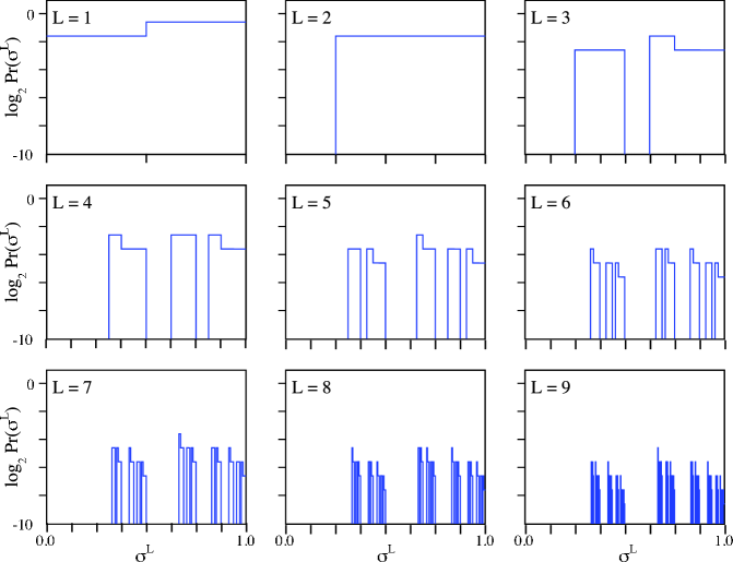
Figure 1: Example of a process language: In the Golden Mean Process, with alphabet $\Sigma=\{0,1\}$, word $00$ and all words containing it have zero probability. All other words have nonzero probability. The logarithm base 2 of the word probabilities is plotted versus the binary string $\sigma^{L}$, represented as base-$2$ real number “$0.\sigma^{L}$”. To allow word probabilities to be compared at different lengths, the distribution is normalized on $[0,1]$—that is, the probabilities are calculated as densities.

III Stochastic Transducers

The process languages developed above require a new kind of finite-state machine to represent them. And so, our immediate goal is to construct a consistent formalism for machines that can recognize, generate, and transform process languages. We refer to the most general ones as stochastic transducers. We will then specialize these transducers into recognizers and generators.

A few comments on various kinds of stochastic transducer introduced by others will help to motivate our approach, which has the distinct goal of representing process languages. Paz defines stochastic sequential machines that are, in effect, transducers [26]. Rabin defines probabilistic automata that are stochastic sequential machines with no output [27]. Neither, though, considers process languages or the “generation” of any language for that matter. Vidal et al define stochastic transducers, though based on a different definition of stochastic language [28]. As a result, their stochastic transducers cannot represent process languages.

III.1 Definition

Our definition of a stochastic transducer parallels Paz’s stochastic sequential machines.

Definition.

A stochastic finite-state transducer (ST) is a tuple $\{S,X,Y,\{T(y|x)\}\}$ where

1. $S$ is a finite set of states, including a start state $s_{0}$.

2. $X$ and $Y$ are finite alphabets of input and output symbols, respectively.

3. $\{T(y|x):x\in X,y\in Y\}$ is a set of square substochastic matrices of $\mathrm{dim}~{}|S|$, one for each output-input pair $y|x$. The matrix entry $T_{ij}(y|x)$ is the conditional probability, when in state $i$ and reading in symbol $x$, of going to state $j$ and emitting symbol $y$.

Generally, a stochastic transducer (ST) operates by reading in symbols that, along with the current state, determine the next state(s) and output symbol(s). At each step a symbol $x\in X$ is read from the input word. The transducer stochastically chooses a transition $T_{ij}(y|x)>0$, emits symbol $y\in Y$, and updates its state from $i$ to $j$. An ST thus maps an input word to one or more output words. Unless otherwise explicitly stated, in our models there is no delay between reading an input symbol and producing the associated output symbols.

STs are our most general model of finitary (and nonquantum) computation. They are structured so that specialization leads to a graded family of models of increasing sophistication.

III.2 Graphical Representation

The set $\{T(y|x)\}$ can be represented as a directed graph $\mathcal{G}(T)$ with the nodes corresponding to states—the matrix row and column indices. An edge connects nodes $i$ and $j$ and corresponds to an element $T_{ij}>0$ that gives the nonzero transition probability from state $i$ to state $j$. Edges are labeled $x|p|y$ with the input symbol $x\in X$, output symbol $y\in Y$, and transition probability $p=T_{ij}(y|x)$. Since an ST associates outputs with transitions, in fact, what we have defined is a Mealy ST, which differs from the alternative Moore ST in which an output is associated with a state [26].

Definition.

A path is a series of edges visited sequentially when making state-to-state transitions with $T_{ij}>0$.

Definition.

A directed graph $\mathcal{G}$ is connected if there is at least one path between every pair of states.

Definition.

A directed graph $\mathcal{G}$ is strongly connected if for every pair of states, $i$ and $j$, there is at least one path from $i$ to $j$ and at least one from $j$ to $i$.

The states in the graph of an ST can be classified as follows, refining the definitions given by Paz [26, p. 85].

Definition.

A state $j$ is a consequent of state $i$ if there is a path beginning at $i$ and ending at $j$.

Definition.

A state is called transient if it has a consequent of which it is not itself a consequent.

Definition.

A state is called recurrent if it has at least one consequent of which it is itself a consequent.

Note that transient and recurrent states can be overlapping sets. We therefore make the following distinctions.

Definition.

A state is called asymptotically recurrent if it is recurrent, but not transient.

Definition.

A state is called transient recurrent if it is transient and recurrent.

Generally speaking, an ST starts in a set of transient states and ultimately transits to one or another of the asymptotically recurrent subsets. That is, there can be more than one set of asymptotically recurrent states. Unless stated otherwise, though, in the following we will consider STs that have only a single set of asymptotically recurrent states.

III.3 Word Probabilities

Before discussing the process languages associated with an ST we must introduce the matrix notation required for analysis. To facilitate comparing classical stochastic models and their quantum analogs, we adapt Dirac’s bra-ket notation: Row vectors $\mathinner{\langle{\cdot}|}$ are called bra vectors; and column vectors $\mathinner{|{\cdot}\rangle}$, ket vectors.

Notation.

Let $\mathinner{|{\eta}\rangle}=(1,1,\ldots,1,1)^{T}$ denote a column vector with $|S|$ components that are all $1$s.

Notation.

Let $\mathinner{\langle{\pi}|}=(\pi_{0},\pi_{1},\ldots,\pi_{|S|-1})$ be a row vector whose components, $0\leq\pi_{i}\leq 1$, give the probability of being in state $i$. The vector is normalized in probability: $\sum_{i=0}^{|S|-1}\pi_{i}=1$. The initial state distribution, with all of the probability concentrated in the start state, is denoted $\mathinner{\langle{\pi^{0}}|}=(1,0,\ldots,0)$.

For a series of $L$ input symbols the action of the corresponding ST is a product of transition matrices:

$$T(y^{L}|x^{L})=T(y_{0}|x_{0})T(y_{1}|x_{1})\cdots T(y_{L-1}|x_{L-1})~{},$$

whose elements $T_{ij}(y^{L}|x^{L})$ give the probability of making a transition from state $i$ to $j$ and generating output $y^{L}$ when reading input $x^{L}$.

Starting in state distribution $\mathinner{\langle{\pi^{0}}|}$, the state distribution after reading in word $x^{L}$ and emitting word $y^{L}$ is

$$\mathinner{\langle{\pi(y^{L}|x^{L})}|}=\mathinner{\langle{\pi^{0}}|}T(y^{L}|x^{L})~{}.$$ (4)

This can then be used to compute the probability of reading out word $y^{L}$ conditioned on reading in word $x^{L}$:

$$\mathrm{Pr}(y^{L}|x^{L})=\mathinner{\langle{\pi(y^{L}|x^{L})|\eta}\rangle}~{}.$$ (5)

IV Stochastic Recognizers and Generators

We are ready now to specialize this general architecture into classes of recognizing and generating devices. In each case we address those aspects that justify our calling them models; viz., we can calculate various properties of the process languages that they represent directly from the machine states and transitions, such as the word distribution and statistical properties that derive from it.

Generally speaking, a recognizer reads in a word and has two possible outputs for each symbol being read in: accept or reject. This differs from the common model [29] of reading in a word of finite length and only at the end deciding to accept or reject. This aspect of our model is a consequence of reading in process languages which are subword closed.

In either the recognition or generation case, we will discuss only models for arbitrarily long, but finite-time observations. This circumvents several technical issues that arise with recognizing and generating infinite-length strings, which is the subject of $\omega$-language theory of Büchi automata [30].

Part of the burden of the following sections is to introduce a number of specializations of stochastic machines. Although it is rarely good practice to use terminology before it is defined, in the present setting it will be helpful when tracking the various machine types to explain our naming and abbreviation conventions now.

In the most general case—in particular, when the text says nothing else—we will discuss, as we have just done, machines. These are input-output devices or transducers and we will denote this in any abbreviation with a capital T. These will be specialized to recognizers, abbreviated R, and generators, denoted G. Within these basic machine types, there will be various alternative implementations. We will discuss stochastic (S) and quantum (Q) versions. Within these classes we will also distinguish the additional property determinism, denoted D.

As noted above, the entire development concerns machines with a finite set of states. And so, we will almost always drop the adjectives “finite-state” and “finitary”, unless we wish to emphasize these aspects in particular.

IV.1 Stochastic Recognizers

Stochastic devices that recognize inputs have been variously defined since the first days of automata theory. Rabin’s probabilistic automata [27], for example, associate a stochastic matrix to each input symbol so that for a given state and input symbol the machine stochastically transitions to a successor state. Accepting an input string $x^{L}$ with cut point $\lambda$ is defined operationally by repeatedly reading in the same string and determining that the acceptance probability was above threshold: $p(x^{L})>\lambda$. Accepting or rejecting with isolated cut point $\lambda$ is defined for some $\delta>0$ with $|p(x^{L})-\lambda|\leq\delta$, respectively.

Here we introduce a stochastic recognizer that applies a variable form of cut-point recognition to process languages with the net effect of representing the word distribution within a uniform tolerance.

One difference between the alternative forms of acceptance is the normalization over equal-length strings for stochastic language recognition. Thus, Rabin’s probabilistic automata do not recognize stochastic languages, but merely assign a number between $0$ and $1$ to each word being read in. The same is true for Paz’s stochastic sequential machines.

Definition.

A stochastic finite-state recognizer (SR) is a stochastic transducer with $|Y|=1$ and $T(y|x)=T(x)$.

One can think of the output symbol as $accept$. If no symbol is output the recognizer has halted and rejected the input.

An SR’s state-to-state transition matrix:

$$T=\sum_{x\in X}T(x)~{},$$ (6)

is a stochastic matrix.

Definition.

An SR accepts a process language $\mathcal{P}$ with threshold $\delta$, if and only if for all $w\in\mathcal{P}$

$$|\mathrm{Pr}(w)-\mathinner{\langle{\pi^{0}|T(w)|\eta}\rangle}|\leq\delta$$ (7)

and for all $w\notin\mathcal{P}$, $\mathinner{\langle{\pi^{0}|T(w)|\eta}\rangle}=0$.

The first criterion for accepting a process language is that all words in the language lead the machine through a series of transitions with positive probability and that words not in the language are assigned zero probability. That is, it accepts the support of the language. The second criterion is that the probability of accepting a word in the language is equal to the word’s probability within a threshold $\delta$. Thus, an SR not only tests for membership in a formal language, it also recognizes a function: the probability distribution of the language. For example, if $\delta=0$ the SR accepts exactly a process language’s word distribution. If $\delta>0$ it accepts the probability distribution with some fuzziness, still rejecting all of the language’s probability-$0$ words. As mentioned before, recognition happens at each time step. This means that in practice the experimenter runs an ensemble of SRs on the same input. The frequency of acceptance can then be compared to the probability of the input string computed from the $T(x)$.

Definition.

The stationary state distribution $\mathinner{\langle{\pi^{s}}|}$, which gives the asymptotic state visitation probabilities, is determined by the left eigenvector of $T(x)$:

$$\mathinner{\langle{\pi^{s}}|}=\mathinner{\langle{\pi^{s}}|}T(x)~{},$$ (8)

normalized in probability: $\sum_{i=0}^{|S|-1}\pi^{s}_{i}=1$.

For a series $x_{0}x_{1}\cdots x_{L-1}$ of input symbols the action of the corresponding SR upon acceptance is a product of transition matrices:

$$T(x^{L})=T(x_{0})T(x_{1})\cdots T(x_{L-1})~{},$$

whose elements $T_{ij}(x^{L})$ give the probability of making a transition from state $i$ to $j$ and generating output $accept$ when reading input $x^{L}$. If the SR starts in state distribution $\mathinner{\langle{\pi^{0}}|}$, the state distribution $\mathinner{\langle{\pi(x^{L})}|}$ after accepting word $x^{L}$ is

$$\mathinner{\langle{\pi(x^{L})}|}=\mathinner{\langle{\pi^{0}}|}T(x^{L})~{}.$$ (9)

In this case, the probability of accepting $x^{L}$ is

$$\mathrm{Pr}(x^{L})=\mathinner{\langle{\pi^{0}|T(x^{L})|\eta}\rangle}~{}.$$ (10)

We have the following special class of SRs.

Definition.

A stochastic deterministic finite-state recognizer (SDR) is a stochastic finite-state recognizer whose substochastic transition matrices $T(x)$ have at most one nonzero element per row.

A word accepted by an SDR is associated with one and only one path. This allows us to give an efficient expression for the word distribution of the language exactly ($\delta=0$) recognized by an SDR:

$$\mathrm{Pr}(x^{L})=T_{s_{0}s_{1}}(x_{0})T_{s_{1}s_{2}}(x_{1})\cdots T_{s_{L-1}s_{L}}(x_{L-1})~{},$$ (11)

where $s_{1}s_{2}\ldots s_{L}$ is the unique series of states along the path selected by $x^{L}$.

There is an important difference here with Eq. (10). Due to determinism, the computational cost for computing the word probability $\mathrm{Pr}(x^{L})$ from SDRs increases only linearly with $L$; whereas it is exponential for SRs.

Figure 2 shows an example of an SDR that recognizes the Golden Mean process language. That is, it rejects any word containing two consecutive $0$s and accepts any other word with nonzero probability. This leads, in turn, to the self-similar structure of the support of the word probability distribution noted in Fig. 1.

A useful way to characterize this property is to list a process language’s irreducible forbidden words—the shortest disallowed words. In the case of the Golden Mean formal language, this list has one member: $\mathcal{F}=\{00\}$. Each irreducible word is associated with a family of longer words containing it. This family of forbidden words forms a Cantor set in the space of sequences, as described above. (Recall Fig. 1.)

If we take the threshold to be $\delta=0$, then the SDR recognizes only the process language shown in Fig. 1. If $\delta=1$, in contrast, the SDR would accept process languages with any distribution on the Golden Mean process words. That is, it always recognizes the language’s support.

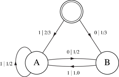
Figure 2: Stochastic deterministic recognizer for the Golden Mean process language of Fig. 1. The edges are labeled $x|p$, where $x\in X$ and $p=T_{ij}(x)$. The start state $\mathinner{\langle{\pi^{0}}|}=(1,0,0)$ is double circled. The reject state and all transitions to it are omitted; as is the output $accept$ on all edges.

One can easily calculate word probabilities and state distributions for the Golden Mean Process using the SDR’s matrix representation.

$$T(0)=\left(\begin{array}[]{ccc}0&0&\tfrac{1}{3}\\ 0&0&\tfrac{1}{2}\\ 0&0&0\end{array}\right)~{}\mathrm{and}~{}T(1)=\left(\begin{array}[]{ccc}0&\tfrac{2}{3}&0\\ 0&\tfrac{1}{2}&0\\ 0&1&0\end{array}\right).$$ (12)

We use Eq. (10) with the start state distribution $\mathinner{\langle{\pi^{0}}|}=(1,0,0)$ to calculate the $L=1$ word probabilities:

$$\mathrm{Pr}(0) =\mathinner{\langle{\pi^{0}|T(0)|\eta}\rangle}=\tfrac{1}{3}~{},$$

$$\mathrm{Pr}(1) =\mathinner{\langle{\pi^{0}|T(1)|\eta}\rangle}=\tfrac{2}{3}~{}.$$

(Eq. (11) would be equally applicable.) At $L=3$ one finds for $x^{3}=011$:

$$\mathrm{Pr}(011)=\mathinner{\langle{\pi^{0}|T(011)|\eta}\rangle}=\mathinner{\langle{\pi^{0}|T(0)T(1)T(1)|\eta}\rangle}=\tfrac{1}{6}.$$

In fact, all $L=3$ words have the same probability, except for $x^{3}=101$, which has a higher probability, $\mathrm{Pr}(101)=\tfrac{1}{3}$, and $x^{3}\in\{000,001,100\}$, for which $\mathrm{Pr}(x^{3})=0$. (Cf. the $L=3$ word distribution in Fig. 1.)

The conditional probability of a $1$ following a $0$, say, is calculated in a similarly straightforward manner:

$$\mathrm{Pr}(1|0)=\frac{\mathrm{Pr}(01)}{\mathrm{Pr}(0)}=\frac{\mathinner{\langle{\pi^{0}|T(0)T(1)|\eta}\rangle}}{\mathinner{\langle{\pi^{0}|T(0)|\eta}\rangle}}=1~{}.$$

Whereas, the probability $\mathrm{Pr}(0|0)$ of a $0$ following a $0$ is zero, as expected.

IV.2 Stochastic Generators

As noted in the introduction, finite-state machines generating strings of symbols can serve as useful models for structure in dynamical systems. They have been used as computational models of classical dynamical systems for some time; see Refs. [31, 17, 32, 33, 19, 34, 14], for example.

As we also noted, automata that only generate outputs are less often encountered in formal language theory [29] than automata operating as recognizers. One reason is that redefining a conventional recognizer to be a device that generates output words is incomplete. A mechanism for choosing which of multiple transitions to take when leaving a state needs to be specified. And this leads naturally to probabilistic transition mechanisms, as one way of completing a definition. We will develop finite-state generators by paralleling the development of SRs.

Definition.

A stochastic finite-state generator (SG) is a stochastic transducer with $|X|=1$.

The input symbol can be considered a clock signal that drives the machine from state to state. The transition matrices can be simplified to $T(y)=T(y|x)$. An SG’s state-to-state transition probabilities are given by the stochastic state-to-state transition matrix:

$$T=\sum_{y\in Y}T(y)~{}.$$ (13)

Word probabilities are calculated as with SRs, save that one exchanges input symbols $x$ with output symbols $y$:

$$\mathrm{Pr}(y^{L})=\mathinner{\langle{\pi^{0}|T(y^{L})|\eta}\rangle}~{}.$$ (14)

We define the following special class of SGs.

Definition.

A stochastic deterministic finite-state generator (SDG) is a stochastic finite-state generator in which each matrix $T(y)$ has at most one nonzero entry per row.

As with SDRs, given the generator’s state and an output symbol, the next state is uniquely determined. Similarly, it is less costly to compute word probabilities:

$$\mathrm{Pr}(y^{L})=T_{s_{0}s_{1}}(y_{0})T_{s_{1}s_{2}}(y_{1})\cdots T_{s_{L-1}s_{L}}(y_{L-1})~{}.$$ (15)

Given an initial state distribution, a sum is taken over states, weighted by their probability. Even so, the computation increases only linearly with $L$. In the following we concentrate on SDGs.

As an example, consider the generator for the Golden Mean process language. Its matrix representation is the same as for the Golden Mean recognizer given in Eqs. (12). Its graphical representation is the same as in Fig. 2, except that the edge labels $x|p$ there should be given as $p|y$. (We return to the relationship between recognizers and equivalent generators shortly.) It turns out this is the smallest generator, but the proof of this will be presented elsewhere.

One can easily calculate word probabilities and state distributions for the Golden Mean Process using the SDG’s matrices. Let us consider a method, different from that used above for SRs, that computes probabilities using the asymptotically recurrent states only. This is done using the stationary state distribution and the transition matrices restricted to the asymptotically recurrent states. The method is useful whenever the start state is not known, but the asymptotic behavior of the machine is. The transition matrices for the SDG, following Eqs. (12), become:

$$T(0)=\left(\begin{array}[]{cc}0&\frac{1}{2}\\ 0&0\end{array}\right)~{}\mathrm{and}~{}T(1)=\left(\begin{array}[]{cc}\frac{1}{2}&0\\ 1&0\end{array}\right).$$ (16)

The stationary state distribution $\mathinner{\langle{\pi^{s}}|}$ is the left eigenvector of the state-to-state transition matrix $T$, Eq. (13): $\mathinner{\langle{\pi^{s}}|}=\mathinner{\langle{\tfrac{2}{3},\tfrac{1}{3}}|}$.

Assuming that the initial state is not known, but the process has been running for a long time, we use Eq. (14) with $\mathinner{\langle{\pi^{s}}|}$ to calculate the $L=1$ word probabilities:

$$\mathrm{Pr}(0) =\mathinner{\langle{\pi^{s}|T(0)|\eta}\rangle}=\tfrac{1}{3}~{},$$

$$\mathrm{Pr}(1) =\mathinner{\langle{\pi^{s}|T(1)|\eta}\rangle}=\tfrac{2}{3}~{}.$$

At $L=3$ one finds for $y^{3}=011$:

$$\mathrm{Pr}(011)=\mathinner{\langle{\pi^{s}|T(011)|\eta}\rangle}=\mathinner{\langle{\pi^{s}|T(0)T(1)T(1)|\eta}\rangle}=\tfrac{1}{6}~{}.$$

All $L=3$ words have the same probability, except for $y^{3}=101$, which has a higher probability, $\mathrm{Pr}(101)=\tfrac{1}{3}$, and $y^{3}\in\{000,001,100\}$, for which $\mathrm{Pr}(y^{3})=0$. (Cf. the $L=3$ distribution in Fig. 1.)

These are the same results found for the Golden Mean Process recognizer. There, however, we used a different initial distribution. The general reason why these two calculations lead to the same result is not obvious, but an explanation would take us too far afield.

As a second example of an SDG consider the Even Process whose language consists of blocks of even numbers of $1$s bounded by $0$s. The substochastic transition matrices for its recurrent states are

$$T(0)=\left(\begin{array}[]{cc}\frac{1}{2}&0\\ 0&0\end{array}\right)~{}\mathrm{and}~{}T(1)=\left(\begin{array}[]{ccc}0&\frac{1}{2}\\ 1&0\end{array}\right)~{}.$$ (21)

The corresponding graph is shown in Fig. 3. Notice that the state-to-state transition matrix $T$ is the same as the previous model of the Golden Mean Process. However, the Even Process is substantially different; and its SDG representation lets us see how. The set of irreducible forbidden words is countably infinite [22]: $\mathcal{F}=\{01^{2k+1}0:~{}k=0,1,2,\ldots\}$. Recall that the Golden Mean Process had only a single irreducible forbidden word $\{00\}$. One consequence is that the words in the Even Process have a kind of infinite correlation: the “evenness” of the length of $1$-blocks is respected over arbitrarily long words. This makes the Even Process effectively non-finite: As long as a sequence of $1$s is produced, memory of the initial state distribution persists. Another difference is that the support of the word distribution has a countable infinity of distinct Cantor sets—one for each irreducible forbidden word. Thus, the Even Process falls into the broader class of finitary processes.

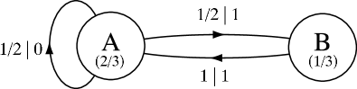
Figure 3: A deterministic generator of the Even Process: Blocks of an even number of $1$s are separated by $0$s. Only the asymptotically recurrent states are shown. Edges are labeled $p\,|\,y$, where $y\in Y$ and $p=T_{ij}(y)$. The numbers in parentheses give a state’s asymptotic probability.

IV.3 Properties

We can now describe the similarities and differences between stochastic and other kinds of recognizers and between the various classes of generators. Let $\mathcal{S}(\mathcal{M})$ denote the stochastic language recognized or generated by automaton $\mathcal{M}$. Let $\mathcal{\mathbf{P}}(C)$ denote the set of stochastic languages generated or recognized by machines in class $C$.

The relationships between the languages associated with the various machine types follow rather directly from their definitions. We swap input and output alphabets and reinterpret the same transition matrices, either as specifying $x|p$ or $p|y$ as required. All, that is, except for the last two results, which may be unexpected.

Proposition 1.

For every SR, $\mathrm{supp}\;\mathcal{S}(SR)$ is a regular language.

Proof.

The graph of an SR, removing the probabilities, defines a finite-state recognizer and accepts, by definition, a regular language [29]. This regular language is the support of $\mathcal{S}(SR)$ by construction.

Proposition 2.

For every SR, $\mathcal{S}(SR)$ is a process language.

Proof.

The first property to establish is that the set of words recognized by an SR is subword closed: if $\mathrm{Pr}(x^{L})>0$, then all $w\in\mathrm{sub}(x^{L})$ have $\mathrm{Pr}(w)>0$. This is guaranteed by definition, since the first input symbol not encountering an allowed transition leads to rejection of the whole input, see the SR definition.

The second property to establish is that the word distribution $\mathrm{Pr}(x^{L})$ is normalized at each $L$. This follows from $T$ in Eq. 6 being stochastic.

Proposition 3.

SGs and SRs generate and recognize, respectively, the same set of languages: $\mathcal{\mathbf{P}}(SG)=\mathcal{\mathbf{P}}(SR)$.

Proof.

Consider SG’s transition matrices $T(y)$ and form a new set $T(x)$ in which $X=Y$. The $T(x)$ define an SR that recognizes $\mathcal{S}(SG)$.

It follows that $\mathcal{\mathbf{P}}(SG)\subseteq\mathcal{\mathbf{P}}(SR)$.

Now consider SR’s transition matrices $T(x)$ and form a new set $T(y)$ in which $Y=X$. The $T(y)$ define an SG that generates $\mathcal{S}(SR)$.

It follows that $\mathcal{\mathbf{P}}(SG)=\mathcal{\mathbf{P}}(SR)$.

Corollary 1.

For every SG, $\mathrm{supp}\;\mathcal{S}(SG)$ is a regular language.

Corollary 2.

For every SG, $\mathcal{S}(SG)$ is a process language.

Corollary 3.

SDGs and SDRs generate and recognize, respectively, the same set of languages: $\mathcal{\mathbf{P}}(SDG)=\mathcal{\mathbf{P}}(SDR)$.

These equivalences are intuitive and expected. They do not, however, hint at the following, which turn on the interplay between nondeterminism and stochasticity.

Proposition 4.

There exists an SG such that $\mathcal{P}(SG)$ is not recognized by any SDR.

Proof.

We establish this by example. Consider the nondeterministic generator in Fig. 4, the Simple Nondeterministic Source (SNS). To show that there is no possible construction of an SDR we argue as follows. If a $0$ appears, then the generator is in state $\mathrm{A}$. Imagine this is then followed by a block $1^{k}$. At each $k$ the generator is in either state $\mathrm{A}$ or $\mathrm{B}$. The probability of seeing a $0$ next is ambiguous (either $0$ or $1/2$) and depends on the exact history of internal states visited. Deterministic recognition requires that a recognizer be in a state in which the probability of the next symbol is uniquely given. While reading in $1$s the recognizer would need a new state for each $1$ connecting to the same state (state $\mathrm{A}$) on a $0$. Since this is true for all $k$, there is no finite-state SDR that recognizes the SNS’s process language.

Ref. [16] gives an SDR for this process that is minimal, but has a countably infinite number of states. Note that $\mathrm{supp}\;{\mathcal{P}(SNS)}$ is the support of the Golden Mean process language.

Corollary 4.

There exists an SR such that $\mathcal{P}(SR)$ is not generated by any SDG.

These propositions say, in essence, that deterministic machines generate or recognize only a subset of the finitary process languages. In particular, Props. 3, 4, and Cor. 3 imply proper containment: $\mathcal{\mathbf{P}}(SDR)\subset\mathcal{\mathbf{P}}(SG)$ and $\mathcal{\mathbf{P}}(SDG)\subset\mathcal{\mathbf{P}}(SR)$. This is in sharp contrast with the standard result in formal language theory: deterministic and nondeterministic automata recognize the same class of languages—the regular languages [29].

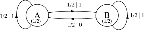
Figure 4: A nondeterministic generator that produces a process language not recognized by any (finite-state) SDR. Only asymptotically recurrent states are shown. Edges are labeled $p\,|\,y$, where $y\in\{0,1\}$ and $p=T_{ij}(y)$.

This ends our development of classical machines and their specializations. We move on to their quantum analogs, following a strategy that is familiar by now.

V Finitary Quantum Processes

As with stochastic processes, the evolution of a quantum system is monitored by a series of measurement outcomes—numbers registered in some way. Each outcome can be taken to be the realization of a random variable. The distribution over sequences of these random variables is what we call a quantum process. We will consider the finitary version of quantum processes in the same sense as used for the classical stochastic processes: The internal resources used during the evolution are finitely specified.

V.1 Quantum States

Quantum mechanics is sometimes viewed as a generalization of classical probability theory with noncommuting probabilities. It is helpful, therefore, to compare classical stochastic automata and quantum automata and, in particular, to contrast the corresponding notions of state. The goal is to appreciate what is novel in quantum automata. The reader should have a working knowledge of quantum mechanics at the level of, say, Ref. [35].

In the classical (stochastic) setting an automaton has internal states $S$ and also a distribution $\mathinner{\langle{\pi}|}$ over them. The distribution itself can be taken to be a “state”, but of what? One interpretation comes from considering how an observer monitors a series of outputs from a stochastic generator and predicts, with each observed symbol, the internal state $s\in S$ the automaton is in. This prediction is a distribution $\mathinner{\langle{\pi}|}$ over the internal states—one that represents the observer’s best guess of the automaton’s current internal state. In this sense the distribution is the state of the best predictor. If $\mathinner{\langle{\pi}|}=(0,\ldots,0,\pi_{i}=1,0,\ldots,0)$, then the observer knows exactly what internal state, $s_{i}\in S$, the automaton is in. For these special cases one can identify state distributions and internal states.

Similarly, there are several kinds of state that one might define for a quantum automaton. Each quantum automaton will consist of internal states and we will take the state of the automaton to be a superposition over them. The central difference with classical (stochastic) automata is that the superposition over internal states is not a probability distribution. In particular, internal states have complex amplitudes and, therefore, they potentially interfere. This, in turn, affects the process language associated with the quantum automaton.

In contrast with quantum automata, the state of a quantum dynamical system depends on the choice of a basis that spans its state space. The state is completely specified by the system’s state vector, a unit vector represented as a sum of basis states that span the state space. However, if one chooses a basis consisting of the eigenstates of an observable and associates them with internal states of quantum automaton, there is a simple correspondence between a state vector of a quantum dynamical system (a superposition of basis states) and a state of a quantum automaton (a superposition over internal states). Thus, we will use the terms internal states (of an automaton) and basis states (of a quantum dynamical system’s state space) interchangeably. By similar reasoning, the state vector (of a quantum dynamical system) and state (of a quantum automaton) will be used interchangeably.

In the vocabulary of quantum mechanics, at any moment in time a given quantum automaton is in a pure state—another label for a superposition over internal states. An observer’s best guess as to the automaton’s current pure state is a probability distribution over state vectors—the so-called mixed state.

It is helpful to imagine a collection of individual quantum automata, each in a (pure) state, that is specified by a distribution of weights. One can also imagine a single quantum automaton being in different pure states at different moments in time. The time-averaged state then is also a mixed state. It is the latter picture that we adopt here.

The fact that a quantum pure state can be a superposition of basis states is regarded as the extra structure of quantum mechanics that classical mechanics does not have. We respect this distinction by building a hierarchy of quantum states that goes from basis states to superpositions of basis states to mixtures of superpositions. The analogous classical-machine hierarchy goes only from internal states to distributions over internal states.

V.2 Quantum Measurement

We now turn to the measurement process, a crucial and also distinctive component in the evolution of a quantum dynamical system, and draw parallels with quantum automata. In setting up an experiment, one makes choices of how and when to measure the state of a quantum system. These choices typically affect what one observes, and in ways that differ radically from classical dynamical systems.

Measurement is the experimental means of characterizing a system in the sense that the observed symbols determine the process language and any subsequent prediction of the system’s behavior. The measurement of a quantum mechanical system is described by a Hermitian operator that projects the current state onto one (or several) of the operator’s eigenstates. After a measurement, the system is, with certainty, in the associated (subset of) eigenstate(s). Such an operator is also called an observable and the eigenvalues corresponding to the eigenstates are the observed measurement outcomes.

To model this situation with a quantum automaton, we identify the states of the automaton with the eigenstates of a particular observable. A measurement is defined through an operator that projects the automaton’s current state vector onto one (or a subset) of its internal (basis) states. The “observed” measurement outcome is emitted as a symbol labeling the transition(s) which enter that internal state (or that subset of states).

VI Quantum Transducers

The study of quantum finite-state automata has produced a veritable zoo of alternative models for language recognition. (These are reviewed below in Section VII.2.) Since we are interested in recognition, generation, and transduction of process languages, we start out defining a generalized quantum-finite state transducer and then specialize. We develop a series of quantum finite-state automaton models that are useful for recognition and generation and, ultimately, for modeling intrinsic computation in finitary quantum processes. It is worth recalling that these quantum finite-state machines form the lowest level of a hierarchy of quantum computational models. Thus, they are less powerful than quantum Turing machines. Nevertheless, as we will see, they exhibit a diversity of interesting behaviors. And, in any case, they represent currently feasible quantum computers.

VI.1 Definition

We define a quantum transducer that corresponds to the standard quantum mechanical description of a physical experiment.

Definition.

A quantum transducer (QT) is a tuple $\{Q,\mathinner{\langle{\psi}|}\in\mathcal{H},X,Y,\mathbf{T}(Y|X)\}$ where

1. $Q=\{q_{i}:i=0,\ldots,n-1\}$ is a set of $n$ internal states.

2. The state vector $\mathinner{\langle{\psi}|}$ lies in an $n$-dimensional Hilbert space $\mathcal{H}$; its initial value is the start state $\mathinner{\langle{\psi^{0}}|}$.

3. $X$ and $Y$ are finite alphabets for input and output symbols, respectively.

4. $\mathbf{T}(Y|X)$ is a set of $n\times n$ transition matrices $\{T(y|x)=U(x)P(y),x\in X,y\in Y\}$ that are products of

   1. a unitary matrix $U(x)$: $U^{\dagger}(x)=U^{-1}(x)$ ($\dagger$ denotes complex transpose); and

   2. a projection operator $P(y)$.

At each time step a quantum transducer ($QT$) reads a symbol $x\in X$ from the input, outputs a symbol $y\in Y$, and updates its state vector $\mathinner{\langle{\psi}|}$ via $T(y|x)$.

The preceding discussion of state leads to the following correspondence between a QT’s internal states and state vectors.

Definition.

One associates an internal state $q_{i}\in Q$ with the eigenstate $\mathinner{\langle{\phi_{i}}|}$ of an observable such that:

1. For each $q_{i}\in Q$ there is a basis vector $\mathinner{\langle{\phi_{i}}|}=(0,\ldots,1,\ldots,0)$ with a $1$ in the $i^{\mathrm{th}}$ component.

2. The set $\{\mathinner{\langle{\phi_{i}}|}:i=0,1,\dots,n-1\}$ spans the Hilbert space $\mathcal{H}$.

Definition.

A state vector $\mathinner{\langle{\psi}|}\in\mathcal{H}$ is a unit vector. It can be expanded in terms of basis states $\mathinner{\langle{\phi_{i}}|}$:

$$\mathinner{\langle{\psi}|}=\sum_{i=0}^{n-1}\mathinner{\langle{\phi_{i}}|}c_{i}~{},$$ (22)

with $c_{i}\in\mathbb{C}$ and $\sum_{i=0}^{n-1}c_{i}^{*}c_{i}=1$.

Identifying internal states $q_{i}$ and basis states $\mathinner{\langle{\phi_{i}}|}$ connects the machine view of a quantum dynamical system with that familiar from standard developments of quantum mechanics. A QT state is given by its current state vector $\mathinner{\langle{\psi}|}$. At each time step a symbol $x$ is read in, which selects a unitary operator $U(x)$. The operator is applied to the state vector and the result is measured via $P(y)$. The output, an eigenvalue of the observable, is symbol $y$.

We describe a QT’s operation via the evolution of a bra (row) vector. We make this notational choice, which is unconventional in quantum mechanics, for two reasons that facilitate comparing classical and quantum automata. First, the state distribution of a classical finite-state machine is given conventionally by a row vector. And second, the graphical meaning of a transition from state $i$ to $j$ is reflected in the transition matrix entries $T_{ij}$, only if one uses row vectors and left multiplication with $T$. This is also convention for stochastic processes.

VI.2 Measurement

The projection operators are familiar from quantum mechanics and can be defined in terms of the internal (basis) states as follows.

Definition.

A projection operator $P(y)$ is the linear operator

$$P(y)=\mathinner{|{\phi_{i}}\rangle}\mathinner{\langle{\phi_{i}}|}~{},$$ (23)

where $\phi_{i}$ is the eigenvector of the observable with eigenvalue $y$. In the case of degeneracy $P(y)$ sums over a complete set $\{i\}$ of mutually orthogonal eigenstates:

$$P(y)=\sum_{\{i\}}\mathinner{|{\phi_{i}}\rangle}\mathinner{\langle{\phi_{i}}|}~{}.$$ (24)

Each $P$ is Hermitian ($P^{\dagger}=P$) and idempotent ($P^{2}=P$).

$\mathbf{P}\equiv\{P(y):y\in Y\cup\{\lambda\}\}$ is the set of projection operators with $\sum_{y\in Y}P(y)={\mathbbm{1}}$, where ${\mathbbm{1}}$ is the identity matrix. $\lambda$ is the null symbol and a placeholder for “no measurement”. We take $P(\lambda)={\mathbbm{1}}$ and do not include it in the calculation of word probabilities, for example. “No measurement” differs from a non-selective measurement where a projection takes place, but the outcome is not detected. The decision whether to perform a measurement or not is considered an input to the QT.

In the eigenbasis of a particular observable the corresponding matrices only have $0$ and $1$ entries. In the following we assume such a basis. In addition, we consider only projective measurements which apply to closed quantum systems. (Open systems will be considered elsewhere.)

In quantum mechanics, one distinguishes between degenerate and non-degenerate measurement operators [36]. A non-degenerate measurement operator projects onto one-dimensional subspaces of $\mathcal{H}$. That is, the eigenvectors of the operator all have distinct eigenvalues. In contrast, the operators associated with a degenerate measurement have degenerate eigenvalues. Such an operator projects onto higher-dimensional subspaces of $\mathcal{H}$. After such a measurement the QT is potentially in a superposition of states $\sum_{i}c_{i}\mathinner{\langle{\phi_{i}}|}$, where $i$ sums over the degenerate set of mutually orthogonal eigenstates. Just as degeneracy leads to interesting consequences in quantum physics, we will see in the examples to follow that degenerate eigenvalues lead to interesting quantum languages.

QTs model a general experiment on a quantum dynamical system. As such they should be contrasted with the sequential machines and transducers of Refs. [37] and [38], respectively, that map the current quantum state onto an output. This mapping, however, is not associated with a measurement interaction and lacks physical interpretation.

VI.3 Evolution and Word Distributions

We can now describe a QT’s operation as it scans its input. Starting in state $\mathinner{\langle{\psi^{0}}|}$ it reads in a symbol $x\in X$ from an input word and updates its state by applying the unitary matrix $U(x)$. Then the state vector is projected with $P(y)$ and renormalized. Finally, symbol $y\in Y$ is emitted. That is, the state vector after a single time-step of a QT is given by:

$$\mathinner{\langle{\psi(y|x)}|} =\frac{\mathinner{\langle{\psi^{0}}|}T(y|x)}{\sqrt{\mathinner{\langle{\psi^{0}|T(y|x)T^{\dagger}(y|x)|\psi^{0}}\rangle}}}$$

$$=\frac{\mathinner{\langle{\psi^{0}}|}U(x)P(y)}{\sqrt{\mathinner{\langle{\psi^{0}|U(x)P(y)U^{\dagger}(x)|\psi^{0}}\rangle}}}~{}.$$ (25)

In the following we drop the renormalization factor in the denominator to enhance readability. It will be mentioned explicitly when a state is not to be normalized.

When a QT reads in a length-$L$ word $x^{L}\in X^{L}$ and outputs a length-$L$ word $y^{L}\in Y^{L}$, the transition matrix becomes

$$T(y^{L}|x^{L})=U(x_{0})P(y_{0})\cdots U(x_{L-1})P(y_{L-1})$$ (26)

and the updated state vector is

$$\mathinner{\langle{\psi(y^{L}|x^{L})}|}=\mathinner{\langle{\psi^{0}}|}T(y^{L}|x^{L})~{}.$$ (27)

Starting the QT in $\mathinner{\langle{\psi^{0}}|}$ the conditional probability $\mathrm{Pr}(y|x)$ of the output symbol $y$ given the input symbol $x$ is calculated from the state vector in Eq. (VI.3), before renormalization:

$$\mathrm{Pr}(y|x)=\mathinner{\langle{{\psi(y|x)}|{\psi(y|x)}}\rangle}~{}.$$ (28)

The probability $\mathrm{Pr}(y^{L}|x^{L})$ of output sequence $y^{L}$ conditioned on input sequence $x^{L}$ is calculated similarly using Eq. (27):

$$\mathrm{Pr}(y^{L}|x^{L})=\mathinner{\langle{{\psi(y^{L}|x^{L})}|{\psi(y^{L}|x^{L})}}\rangle}~{}.$$ (29)

VI.4 Properties

We draw out several properties of QTs on our way to understanding their behavior and limitations.

Proposition 5.

A QT’s output alphabet size is bounded: $|Y|\leq\dim(\mathcal{H})$.

Proof.

This follows from the QT definition since output symbols are directly associated with eigenvalues. The number of eigenvalues is bounded by the dimension of the Hilbert space.

Many properties of QTs are related to a subclass of STs, those with doubly stochastic transition matrices. Given this, it is useful to recall the relationship between unitary and doubly stochastic matrices.

Definition.

Given a unitary matrix $U$, matrix $M$ with $M_{ij}=|U_{ij}|^{2}$ is called a unistochastic matrix.

A unistochastic matrix is doubly stochastic, which follows from the properties of unitary matrices. Compared to a stochastic transducer, a QT’s structure is constrained through unitarity and this is reflected in its architecture. A path exists between node $i$ and node $j$ when $M_{ij}>0$. An equivalent description of a quantum transducer is given by its graphical representation.

Recalling the types of graph state defined in Sec. III.2, we find that only a subset occur in QTs. Specifically, a QT has no transient states.

Proposition 6.

Every node $i$ of $\mathcal{G}$(QT), if connected to a set of nodes $j\neq i$, is a member of a strongly connected set.

Proof.

Given that one path exists from (say) $i$ to $j$, we must show that the reverse one exists, going from $j$ to $i$. According to the definition of a path it is sufficient to show this for the unistochastic matrix $M_{ij}=|U_{ij}|^{2}$. A doubly stochastic matrix can always be expressed as a linear combination of permutation matrices. Thus, any vector $(0,0,\dots,1,\dots)$ with only one $1$ entry can be permuted into any other vector with only one $1$ entry. This is equivalent to saying that, if there is a path from node $i$ to $j$ there is a path from $j$ to $i$.

The graph properties of a unitary matrix mentioned here should be compared with those discussed by Severini [39] and others. The graph of a finite-state machine specified by a unitary matrix is a directed graph, or digraph. A digraph vertex is a source (sink) if it has no ingoing (no outgoing) arcs. A digraph vertex is isolated if it is not joined to another. Ref. [39] characterizes these machines by assuming their digraphs have no isolated nodes, no sinks, and no sources. Given the preceding proposition the nonexistence of sinks or sources follows simply from assuming no isolated nodes.

One concludes that QT graphs are a limited subset of digraphs, namely the strongly connected ones. Furthermore, there is a constraint on incoming edges to a node.

Proposition 7.

All incoming transitions to an internal state are labeled with the same output symbol.

Proof.

Incoming transitions to internal state $q_{i}$ are labeled with output symbol $y$ if $\mathinner{\langle{\phi_{i}}|}$ has eigenvalue $y$. Every eigenstate has a unique eigenvalue, and so the incoming transitions to any particular state $q_{i}$ are labeled with the same output symbol representing one eigenvalue.

Proposition 8.

A QT’s transition matrices $T(y|x)$ uniquely determine the unitary matrices $U(x)$ and the projection operators $P(y)$.

Proof.

Summing the $T(y|x)$ over all $y$ for each $x$ yields the unitary matrices $U(x)$:

$$\sum_{y\in Y}T(y|x)=\sum_{y\in Y}U(x)P(y)=U(x)~{}.$$ (30)

The $P(y)$ are obtained, from any of the $U(x)$, through the inverse of $U^{-1}(x)=U^{\dagger}(x)$:

$$P(y)=U^{\dagger}(x)T(y|x)~{}.$$ (31)

Definition.

A QT is reversible if the automaton defined by the transpose of each $U(x)$ and $P(y)$ is also a QT.

Proposition 9.

QTs are reversible.

Proof.

The transpose of a unitary matrix is unitary. The transpose of a projection operator is the operator itself.

Graphically, the reversed QT is obtained by simply switching the direction of the edges. This produces a transducer with the transition amplitudes $T_{ji}$, formerly $T_{ij}$. The original input and output symbols, which labeled ingoing edges to state $q_{i}$, remain unchanged. Therefore, in general, the languages generated by a QT and its reverse are not the same. By way of contrast, this simple operation applied to an ST does not, in general, yield another ST. A simple way to summarize these properties is that a QT forms a group, an ST forms a semi-group.

VII Quantum Recognizers and Generators

The quantum transducer is our most general construct, describing a quantum dynamical process in terms of inputs and outputs. We will now specialize quantum transducers into recognizers and generators. We do this by paralleling the strategy adopted for developing classes of stochastic transducers. For each machine class we first give a general definition and then specialize, for example, yielding deterministic variants. We establish a number of properties for each type and then compare their descriptive powers in terms of the process languages each class can recognize or generate. The results are collected together in a computational hierarchy of finitary stochastic and quantum processes.

VII.1 Quantum Recognizers

Quantum finite-state machines are almost exclusively discussed as recognizing devices. Following our development of a consistent set of quantum finite-state transducers, we can now introduce quantum finite-state recognizers as restrictions of QTs and compare these with alternative models of quantum recognizers. Since we are interested in the recognition of process languages our definition of quantum recognizers differs from those introduced elsewhere; see Sec. VII.2 below. The main difference is the recognition of a process language including its word distribution. The restrictions that will be imposed on a QT to achieve this are similar to those of the stochastic recognizer.

Definition.

A quantum finite-state recognizer (QR) is a quantum transducer with $|Y|=1$ and $T(y|x)=UP(x)\equiv T(x)$.

One can think of the output symbol $y$ as $accept$. The condition for accepting a symbol is, then,

$$\mathrm{Pr}(x)=\mathinner{\langle{\psi^{0}|T(x)T^{\dagger}(x)|\psi^{0}}\rangle}~{}.$$ (32)

If no symbol is output the recognizer has halted and rejected the input. Operationally, recognition works as it does in the classical setting. An experimenter runs an ensemble of QRs on the same input. The frequency of acceptance can then be compared to the probability of the input string computed using the $T(x)$.

Definition.

A QR accepts a process language $\mathcal{P}$ with word-probability threshold $\delta$, if and only if for all $w\in\mathcal{P}$

$$\left|\mathrm{Pr}(w)\!-\!\mathinner{\langle{\psi^{0}|T(w)T^{\dagger}(w)|\psi^{0}}\rangle}\right|\leq\delta$$ (33)

and for all $w\notin\mathcal{P}$, $\mathinner{\langle{\psi^{0}|T(w)T^{\dagger}(w)|\psi^{0}}\rangle}=0$.

Acceptance or rejection happens at each time step.

We also have deterministic versions of QRs.

Definition.

A quantum deterministic finite-state recognizer (QDR) is a quantum recognizer with transition matrices $T(x)$ that have at most one nonzero element per row.

VII.2 Alternatives

Quantum finite automata were introduced by several authors in different ways, and they recognize different classes of languages. To our knowledge the first mention of quantum automata was made by Albert in 1983 [40]. Albert’s results have been subsequently criticized by Peres as being based on an inadequate notion of measurement [41].

Kondacs and Watrous introduced 1-way and 2-way quantum finite-state automata [42]. The $1$-way automata read symbols once and from left to right (say) in the input word. Their 2-way automata scan the input word many times moving either left to right or right to left. The automata allow for measurements at every time step, checking for acceptance, rejection, or continuation. They show that a 2-way QFA can recognize all regular languages and some nonregular languages. 1-way QFA are less powerful: They can only recognize a subset of the regular languages. A more powerful generalization of a 1-way QFA is a 1-way QFA that allows mixed states, introduced by Aharonov et al [43]. They also allow for nonunitary evolution. Introducing the concept of mixed states simply adds classical probabilities to quantum probabilities and is inherent in our model of QTs.

The distinctions between these results and the QRs introduced here largely follow from the difference between regular languages and process languages. Thus, the result in Ref. [42] that no $1$-way quantum automaton can recognize the language $(0+1)^{*}0$, does not apply to QTs. It clearly is a regular language, but not a process language. Also, the result by Bertoni and Carpentieri that quantum automata can recognize nonregular languages, does not apply here [44]. They find that a quantum automaton that is measured only after the whole input has been read in can recognize a nonregular language. A QR, however, applies measurement operators for every symbol that is being read in.

Moore and one of the authors introduced 1-way quantum automata (without using the term “1-way”) [45]. It is less powerful than the 1-way automata of Kondacs and Watrous, since it allows only for a single measurement after the input has been read in. They also introduced a generalized quantum finite-state automaton whose transition matrices need not be unitary, in which case all regular languages are recognized. A type of quantum transducer mentioned earlier, a quantum sequential machine was introduced by Gudder [37]. The link, however, between machine output and quantum physical measurement is missing. Freivalds and Winter introduced quantum transducers [38] that at each step perform a measurement to determine acceptance, rejection, or continuation of the computation. In addition, they map the current quantum state onto an output. Here too, the mapping is not associated with a measurement interaction and lacks physical interpretation.

These alternative models for quantum automata appear to be the most widely discussed. There are others, however, and so the above list is by no means complete. Our motivation to add yet another model of quantum finite-state transducer and recognizer to this list is the inability of the alternatives to recognize or process languages that represent quantum dynamical systems subject to repeated measurement.

VII.3 Quantum Generators

We now introduce quantum finite-state generators as restrictions of QTs and as a complement to recognizers. They serve as a representation for the behavior of autonomous quantum dynamical systems. In contrast to quantum finite-state recognizers, quantum finite-state generators appear to not have been discussed before. A quantum generator is a QT with only one input. As in the classical case, one can think of the input as a clock signal that drives the machine through its transitions.

Definition.

A quantum finite-state generator (QG) is a quantum transducer with $|X|=1$.

At each step it makes a transition from one state to another and emits a symbol. As in the classical case there are nondeterministic (just implicitly defined) and deterministic QGs.

Definition.

A quantum deterministic finite-state generator (QDG) is a quantum generator in which each matrix $T(y)$ has at most one nonzero entry per row.

Interestingly, there is a mapping from a given QDG to a classical automaton.

Definition.

Given a QDG $\mathcal{M}=\{U,P(y)\}$, the equivalent (classical) SDG $\mathcal{M}^{\prime}=\{T(y)\}$ has unistochastic state-to-state transition matrix $T$ with components $T_{ij}=[U_{ij}]^{2}$.

We leave the technical interpretation of “equivalent” to Thm. 2 below.

As mentioned earlier, in quantum mechanics one distinguishes between degenerate and non-degenerate measurements. Having introduced the different types of quantum generators, we can now make a connection to degenerate measurements.

Definition.

A quantum complete finite-state generator (QCG) is a quantum generator observed via non-degenerate measurements.

In order to average over observations, we must extend the formalism of quantum automata to describe distributions over state vectors. Recalling the notions of state discussed in Section V.1, this means we need to describe mixed states and their evolution.

Let a system be described by a state vector $\mathinner{\langle{\psi_{i}}|}$ at time $t$. If we do not know the exact form of $\mathinner{\langle{\psi_{i}}|}$ but only a set of possible $\mathinner{\langle{\psi_{i}}|},~{}i=0,...,k-1$, then we give the best guess as to the system’s state in terms of a statistical mixture of the $\mathinner{\langle{\psi_{i}}|}$. This statistical mixture is represented by a density operator $\rho$ with weights $p_{i}$ assigned to the $\mathinner{\langle{\psi_{i}}|}$:

$$\rho=\sum_{i=0}^{k-1}p_{i}\mathinner{|{\psi_{i}}\rangle}\mathinner{\langle{\psi_{i}}|}~{}.$$ (34)

The main difference from common usage of “mixed state” is that we compare the same state over time; whereas, typically different systems are compared at a single time. Nevertheless, in both cases, the density matrix formalism applies.

VII.4 Properties

With this notation in hand, we can now establish a number of properties of quantum machines.

Definition.

A QG’s stationary state $\rho^{s}$ is the mixed state that is invariant under unitary evolution and measurement:

$$\rho^{s}=\sum_{y\in Y}P(y)U^{\dagger}\rho^{s}UP(y)~{}.$$ (35)

$\rho^{s}$ is the mixed state which the quantum machine is in on average, since we are describing a single system that is always in a pure state. The stationary state is therefore the best guess of an observer ignorant of the machine’s state.

Theorem 1.

A QG’s stationary state is the maximally mixed state:

$$\rho^{s}=n^{-1}\sum_{i=0}^{n-1}\mathinner{|{\phi_{i}}\rangle}\mathinner{\langle{\phi_{i}}|}=\mathbbm{1}/n~{}.$$ (36)

Proof.

Since the $\mathinner{\langle{\phi_{i}}|}$ are basis states, $\rho^{s}$ is a diagonal matrix equal to the identity multiplied by a factor. Recall that the stationary distribution of a Markov chain with doubly stochastic transition matrix is always uniform [46]. And so, we have to establish that $\rho^{s}$ is an invariant distribution:

$$\rho^{s} =\sum_{y\in Y}P(y)U^{\dagger}\rho^{s}UP(y)$$ (37)

$$=n^{-1}\sum_{y\in Y}P(y)U^{\dagger}UP(y)$$ (38)

$$=n^{-1}\sum_{y\in Y}P(y)=\mathbbm{1}/n~{}.$$ (39)

Now we can calculate the asymptotic symbol probabilities, using the density matrix formalism for computing probabilities of measurement outcomes [47], and $\rho^{s}$.

Proposition 10.

A QG’s symbol distribution depends only on the dimensions of the projection operators and the Hilbert space.

Proof.

Denote the trace operator by $\mathrm{tr}$, then we have

$$\mathrm{Pr}(y) =\mathrm{tr}\left(T^{\dagger}(y)\rho^{s}T(y)\right)$$

$$=n^{-1}\mathrm{tr}\left(T^{\dagger}(y)\mathbbm{1}T(y)\right)$$

$$=n^{-1}\mathrm{tr}\left(P^{\dagger}(y)U^{\dagger}UP(y)\right)$$

$$=n^{-1}\mathrm{tr}\left(P^{\dagger}(y)\mathbbm{1}P(y)\right)$$

$$=n^{-1}\mathrm{tr}\left(P(y)\right)$$

$$=n^{-1}\mathrm{dim}\;P(y)~{}.$$ (40)

Although the single-symbol distribution is determined by the dimension of the subspaces onto which the $P(y)$ project, distributions of words $y^{L}$ with $L>1$ are not similarly restricted. The asymptotic word probabilities $\mathrm{Pr}(y^{L})$ are:

$$\mathrm{Pr}(y^{L})=\mathrm{tr}\left(T^{\dagger}(y^{L})\rho^{s}T(y^{L})\right)~{}.$$ (41)

No further simplification is possible for the general case.

Analogous results follow for QRs, except that the calculations are suitably modified to use $T(x)$.

VII.5 Finitary Process Hierarchy

To better appreciate what these machines are capable of we amortize the effort in developing the preceding results to describe the similarities and differences between quantum recognizers and generators, as well as between stochastic and quantum automata. We collect the results, give a summary and some interpretation, and present a road map (Fig. 5) that lays out the computational hierarchy of finitary quantum processes. As above, $\mathcal{S}(M)$ denotes the stochastic language associated with machine or machine type $M$ and $\mathcal{\mathbf{P}}(C)$, the set of stochastic languages generated or recognized by all machines in class $C$.

Proposition 11.

QCGs are deterministic.

Proof.

Since all projection operators have dimension one, all transition matrices have at most one nonzero element per row. This is the condition for being a QDG.

Non-degenerate measurements always define a QDG. There are degenerate measurements, however, that also can lead to QDGs, as we will show shortly. One concludes that $\mathcal{\mathbf{P}}(QCG)\subset\mathcal{\mathbf{P}}(QDG)$.

We now show that for any QDG there is an SDG generating the same stochastic language. Thereby we establish observational equivalence between the different classes of machine.

Theorem 2.

Every $\mathcal{S}(QDG)$ is generated by some SDG: $\mathcal{\mathbf{P}}(QDG)\subseteq\mathcal{\mathbf{P}}(SDG)$.

Proof.

We show that the SDG generating $\mathcal{S}(QDG)$ is the equivalent SDG, as defined in Sec. VII.3, and that the QDG $\mathcal{M}$ and its equivalent SDG $\mathcal{M}^{\prime}$ generate the same word distribution and so the same stochastic language.

The word probabilities $\mathrm{Pr}_{\mathcal{M}}(y^{L})$ for $\mathcal{M}$ are calculated using Eq. (41) and the QDG’s transition matrices $T_{\mathcal{M}^{\prime}}$:

$$\mathrm{Pr}_{\mathcal{M}}(y^{L}) =\mathrm{tr}\left(T_{\mathcal{M}}^{\dagger}(y^{L})\rho^{s}T_{\mathcal{M}}(y^{L})\right)$$

$$=n^{-1}\mathrm{tr}(T^{\dagger}T)$$

$$=n^{-1}\sum_{i}[T^{\dagger}T]_{ii}$$

$$=n^{-1}\sum_{i}\sum_{j}T_{ij}^{\dagger}T_{ji}$$

$$=n^{-1}\sum_{ij}T_{ij}^{2}~{}.$$

The word probabilities $\mathrm{Pr}_{M^{\prime}}(y^{L})$ for $M^{\prime}$ are calculated using Eq. (14) and the SDG’s transition matrices $T_{\mathcal{M}}$:

$$\mathrm{Pr}_{\mathcal{M}^{\prime}}(y^{L}) =\mathinner{\langle{\pi^{0}|T_{{\mathcal{M}}^{\prime}}(y^{L})|\eta}\rangle}$$

$$=\sum_{i=0}^{n-1}\left(\pi^{0}_{i}\sum_{j}(T_{{\mathcal{M}}^{\prime}}(y^{L}))_{ij}\right)$$

$$=n^{-1}\sum_{i,j=0}^{n-1}(T_{{\mathcal{M}}^{\prime}}(y^{L}))_{ij}~{}.$$ (42)

Since $(T_{\mathcal{M}}(y^{L}))_{ij}^{2}=(T_{\mathcal{M}^{\prime}}(y^{L}))_{ij}$, from the definition of an equivalent SDG, the claim follows.

More than one QDG can be observationally equivalent to a given SDG. The reason for this to occur is that the quantum mechanical phases of the transition amplitudes cancel in the transformation from a QDG.

We can now easily characterize languages produced by QDGs.

Corollary 5.

For every QDG, $\mathrm{supp}\;~{}\mathcal{S}(QDG)$ is a regular language.

Proof.

This follows directly from Thm. 2 and Cor. 1.

Corollary 6.

For every QDG, $\mathcal{S}(QDG)$ is a process language.

Proof.

This follows directly from Thm. 2 and Cor. 2.

With this we can begin to compare the descriptive power of the different machine types.

Proposition 12.

QGs and QRs are equivalent: They recognize and generate the same set of stochastic languages, respectively: $\mathcal{\mathbf{P}}(QG)=\mathcal{\mathbf{P}}(QR)$.

Proof.

Consider QG’s transition matrices $T(y)=UP(y)$ and form a new set $T(x)=UP(x)$ in which $P(x)=P(y)$, associating the QR’s input $X$ with the QG’s output $Y$. The $T(x)$ define a QR that recognizes $\mathcal{S}(QG)$. It follows that $\mathcal{\mathbf{P}}(QG)\subseteq\mathcal{\mathbf{P}}(QR)$.

Now consider QR’s transition matrices $T(x)=UP(x)$ and form a new set $T(y)$ in which $P(y)=P(x)$, associating inputs and outputs as above. The $T(y)$ define a QG that generates $\mathcal{S}(QR)$.

It follows that $\mathcal{\mathbf{P}}(QG)=\mathcal{\mathbf{P}}(QR)$.

Corollary 7.

QDGs and QDRs are equivalent: They recognize and generate the same set of stochastic languages, respectively: $\mathcal{\mathbf{P}}(QDG)=\mathcal{\mathbf{P}}(QDR)$.

Proof.

Prop. 12’s proof goes through if one restricts to deterministic machines.

Corollary 8.

For every QDR, $\mathrm{supp}\;~{}\mathcal{S}(QDR)$ is a regular language.

Proof.

This follows directly from Cor. 1 and Cor. 7.

Corollary 9.

For every QDR, $\mathcal{S}(QDR)$ is a process language.

Proof.

This follows directly from Cor. 6 and Cor. 7.

Proposition 13.

There exists an SDG such that $\mathcal{P}(SDG)$ is not generated by any QDG.

Proof.

The process language generated by the SDG given by $T(0)=\left(\tfrac{1}{\sqrt{2}}\right)$ and $T(1)=\left(1-\tfrac{1}{\sqrt{2}}\right)$ (a biased coin) cannot be generated by any QDG. According to Prop. 10 $\mathrm{Pr}(y)=n^{-1}\mathrm{dim}P(y)$, which is a rational number, whereas $\mathrm{Pr}(y)$ for the above biased coin is irrational.

Corollary 10.

$\mathcal{\mathbf{P}}(QDG)\subset\mathcal{\mathbf{P}}(SDG)$.

Proof.

From Thm. 2 and Prop. 13.

Corollary 11.

$\mathcal{\mathbf{P}}(QDR)\subset\mathcal{\mathbf{P}}(SDR)$:

Proof.

From Cor. 3, Cor. 7, Thm. 2, and Prop. 13.

At this point it is instructive to graphically summarize the relations between recognizer and generator classes. Figure 5 shows a machine hierarchy in terms of sets of languages recognized or generated. The class of QCGs is at the lowest level. This is contained in the class of QDGs and QDRs. The languages they generate or recognize are properly included in the set of languages generated or recognized by classical deterministic machines—SDGs and SDRs. These, in turn, are included in the set of languages recognized or generated by classical nondeterministic machines, SGs and SRs, as well as QRs and QGs.

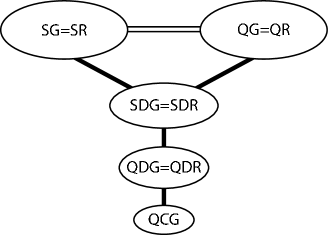
Figure 5: Finitary process language hierarchy: Each circle represents the set of process languages recognized or generated by the inscribed machine class. Increasing height indicates proper containment; machine classes at the same height are not directly comparable. The hierarchy summarizes the theorems, propositions, and corollaries in Secs. IV.3 and VII.5.

The preceding results serve to indicate how portions of the finitary process hierarchy are organized. However, there is still more to understand. For example, the regularity of the support of finitary process languages, the hierarchy’s dependence on acceptance threshold $\delta$, and the comparability of stochastic and quantum nondeterministic machines await further investigation.

VIII Quantum Generators and Finitary Processes: Examples

To appreciate what can be done with quantum machines, we will illustrate various features of QTs by modeling several prototype quantum dynamical systems. We start out with deterministic QGs, building one to model a physical system, and end on an example that illustrates a nondeterministic QT.

VIII.1 Two-State Quantum Processes

According to Prop. 10 the symbol distribution generated by a QG only depends on the dimension of the projection operator and the dimension of the Hilbert space. What are the consequences for two-state QGs? First of all, according to Cor. 5 the maximum alphabet size is $2$. The corresponding projection operators can either have dimension $2$ (for a single-letter alphabet) or dimension $1$ for a binary alphabet. The only symbol probabilities possible are $\mathrm{Pr}(y)=1$ for the single-letter alphabet and $\mathrm{Pr}(y)=1/2$ for a binary alphabet. So one can set aside the single-letter alphabet case as too simple.

We also see that a binary-alphabet two-state QDG can produce only a highly restricted set of process languages. It is illustrative to look at the possible equivalent SDGs. Their state-to-state transition matrices are given by

$$T=\left(\begin{array}[]{cc}p&1-p\\ 1-p&p\end{array}\right)~{},$$ (43)

with $p\in\{0,1/2,1\}$.

For $p=1/2$, for example, this is the fair coin process. It becomes immediately clear that the Golden Mean and the Even processes, which are modeled by two-state classical automata, cannot be represented with a two-state QDG. (The three-state models are given below.)

VIII.1.1 Iterated Beam Splitter

Let’s consider a physical two-state process and build a quantum generator for it.

The iterated beam splitter is an example that, despite its simplicity, makes a close connection with real experiment. Figure 6 shows the experimental apparatus. Photons are sent through a beam splitter (thick dashed line), producing two possible paths. The paths are redirected by mirrors (thick horizontal solid lines) and recombined at a second beam-splitter. From this point on the same apparatus is repeated indefinitely to the right. After the second beam-splitter there is a third and a fourth and so on. Single-photon quantum nondemolition detectors are located along the paths, between every pair of beam-splitters. One measures if the photon travels in the upper path and the other determines if the photon follows the lower path.

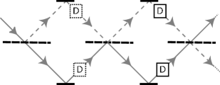
Figure 6: Experimental set-ups for the iterated beam splitter: Solid lines are mirrors; beam splitters, horizontal dashed lines. Photon nondemolition detectors, marked as D, are placed between every pair of beam splitters. Under measurement protocol I all detectors are in operation; under protocol II only the solid-line detectors are activated. The apparatus is repeated indefinitely to the right.

This is a quantum dynamical system: a photon passing repeatedly through various beam splitters. It has a two-dimensional state space with two eigenstates—“above” and “below”. Its behavior is given by the evolution of a state vector $\mathinner{\langle{\psi}|}$. The overall process can be represented in terms of a unitary operation for the beam splitter and projection operators for the detectors. The unitary operator for the beam splitter is the Hadamard matrix $U_{H}$:

$$U_{H}=\frac{1}{\sqrt{2}}\left(\begin{array}[]{cc}1&1\\ 1&-1\end{array}\right)~{}.$$ (44)

The measurement operators have the following matrix representation in the experiment’s eigenbasis:

$$P(0)=\left(\begin{array}[]{cc}1&0\\ 0&0\end{array}\right)~{}\mathrm{and}~{}P(1)=\left(\begin{array}[]{cc}0&0\\ 0&1\end{array}\right)~{},$$ (45)

where the measurement symbol $0$ stands for “above” and symbol $1$ stands for “below”.

Before we turn to constructing a quantum finite-state generator to model this experiment we can understand intuitively the sequence of outcomes that results from running the experiment for long times. If entering the beam splitter from above, the detectors record the photon in the upper or lower path with equal probability. Once the photon is measured, though, it is in that detector’s path with probability $1$. And so it enters the beam splitter again via only one of the two possible paths. Thus, the second measurement outcome will have the same uncertainty as the first: the detectors report “above” or “below” with equal probability. The resulting sequence of outcomes after many beam splitter passages is simply a random sequence. Call this measurement protocol I.

Now consider altering the experiment slightly by removing the detectors after every other beam splitter. In this configuration, call it protocol II, the photon enters the first beam splitter, does not pass a detector and interferes with itself at the next beam splitter. That interference, as we will confirm shortly, leads to destructive interference of one path after the beam splitter. The photon is thus in the same path after the second beam splitter as it was before the first beam splitter. A detector placed after the second beam splitter therefore reports with probability $1$ that the photon is in the upper path, if the photon was initially in the upper path. If it was initially in the lower path, then the detector reports that it is in the upper path with probability $0$. The resulting sequence of upper-path detections is a very predictable sequence, compared to the random sequence from protocol I.

We now construct a QG for the iterated-beam splitter using the matrices of Eqs. (44)-(45) and the stationary state of Eq. (36). The output alphabet consists of two symbols denoting detection “above” or “below”: $Y=\{0,1\}$. The set of states consists of the two eigenstates of the system “above” and “below”: $Q=\{A,B\}$. The transition matrices are:

$$T(0)=U_{H}P(0) =\frac{1}{\sqrt{2}}\left(\begin{array}[]{cc}1&0\\ 1&0\end{array}\right)~{},$$ (46c)

$$T(1)=U_{H}P(1) =\frac{1}{\sqrt{2}}\left(\begin{array}[]{cc}0&1\\ 0&-1\end{array}\right)~{}.$$ (46f)

The resulting QG turns out to be deterministic, as can be seen from its graphical representation, shown in Fig. 7.

The word distribution for the process languages generated by protocols I and II are obtained from Eq. (41). Word probabilities for protocol I (measurement at each time step) are, to give some examples:

$$\mathrm{Pr}(0) =n^{-1}\mathrm{dim}(P(0))=\frac{1}{2}~{},$$ (47a)

$$\mathrm{Pr}(1) =n^{-1}\mathrm{dim}(P(1))=\frac{1}{2}~{},$$ (47b)

$$\mathrm{Pr}(00) =\mathrm{tr}\left(T^{\dagger}(0)T^{\dagger}(0)\rho^{s}T(0)T(0)\right)=\frac{1}{4}~{},$$ (47c)

$$\mathrm{Pr}(01) =\mathrm{Pr}(10)=\mathrm{Pr}(11)=\frac{1}{4}~{}.$$ (47d)

Continuing the calculation for longer words shows that the word distribution is uniform at all lengths $\mathrm{Pr}(y^{L})=2^{-L}$.

For protocol II (measurement every other time step) we find:

$$\mathrm{Pr}(0) =\mathrm{tr}\left(T^{\dagger}(\lambda 0)\rho^{s}T(\lambda 0)\right)=\frac{1}{2}~{},$$ (48a)

$$\mathrm{Pr}(1) =\mathrm{tr}\left(T^{\dagger}(\lambda 1)\rho^{s}T(\lambda 1)\right)=\frac{1}{2}~{},$$ (48b)

$$\mathrm{Pr}(00) =\mathrm{tr}\left(T^{\dagger}(\lambda 0\lambda 0)\rho^{s}T(\lambda 0\lambda 0)\right)=\frac{1}{2}~{},$$ (48c)

$$\mathrm{Pr}(11) =\mathrm{tr}\left(T^{\dagger}(\lambda 1\lambda 1)\rho^{s}T(\lambda 1\lambda 1)\right)=\frac{1}{2}~{},$$ (48d)

$$\mathrm{Pr}(10) =\mathrm{Pr}(01)=0~{}.$$ (48e)

If we explicitly denote the output at the unmeasured time step as $\lambda$, the sequence $11$ turns into $\lambda 1\lambda 1$, as do the other sequences in protocol II. As one can see, the word probabilities calculated from the QDG agree with our earlier intuitive conclusions.

Figure 7: Quantum finite-state machine for the iterated beam splitter: The resulting symbol sequences are statistically identical to the sequences obtained with the measurement protocols I and II shown in Fig. 6. When no measurement is made, transitions along all edges occur.

Comparing the iterated beam splitter QDG to its classically equivalent SDG reveals several crucial differences in performance. Following the recipe from Sec. VII.5, on how to build an SDG from a QDG, gives the classical generator shown in Fig. 8(a). Its transition matrices are:

$$T(0)=\frac{1}{2}\left(\begin{array}[]{cc}1&0\\ 1&0\end{array}\right)~{}\mathrm{and}~{}T(1)=\frac{1}{2}\left(\begin{array}[]{cc}0&1\\ 0&1\end{array}\right)~{}.$$ (49)

The symbol sequence generated by this SDG for protocol I is the uniform distribution for all lengths, as can be easily verified using Eq. (14) or, since it is deterministic, Eq. (15). This is equivalent to the language generated by the QDG under protocol I. However, the probability distribution of the sequences for the generator under protocol II, ignoring every second output symbol, is still the uniform distribution for all lengths $L$. This could not be more different from the language generated by the QDG under protocol II.

The reason is that the classical machine is unable to capture the interference effects present in experimental protocol II. A second SDG has to be constructed from the QDG’s transition matrices for set-up II. This is done by carrying out the matrix product first and then forming its equivalent SDG. The result is shown Fig. 8(b). Its transition matrices are:

$$T(0)=\frac{1}{2}\left(\begin{array}[]{cc}1&0\\ 0&0\end{array}\right)~{}\mathrm{and}~{}T(1)=\frac{1}{2}\left(\begin{array}[]{cc}0&0\\ 0&1\end{array}\right)~{}.$$ (50)

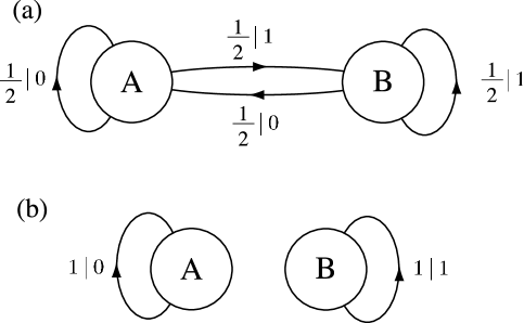
Figure 8: Classical deterministic generators for the iterated beam splitter: (a) Protocol I and (b) protocol II, $\mathnormal{p}=2$. (Cf. Fig. 6.)

The two classical SDGs are clearly (and necessarily) different. Thus, a single QG can model a quantum system’s dynamics for different measurement protocols. Whereas an SG only captures the behavior of each individual experimental set-up. This simple example serves to illustrate the utility of QGs over SGs in modeling the behavior of quantum dynamical systems.

VIII.2 Three-State Quantum Processes

VIII.2.1 Golden Mean Quantum Machine

Recall the classical Golden Mean generator of Sec. IV.2. A QDG, which generates the same process language, is shown in Fig. 9. Consider a spin-$1$ particle subject to a magnetic field that rotates its spin. The state evolution can be described by the unitary matrix

$$U=\left(\begin{array}[]{ccc}\frac{1}{\sqrt{2}}&\frac{1}{\sqrt{2}}&0\\ 0&0&-1\\ -\frac{1}{\sqrt{2}}&\frac{1}{\sqrt{2}}&0\end{array}\right)~{},\\$$ (51)

which is a rotation in $\mathbb{R}^{3}$ around the y-axis by angle $\tfrac{\pi}{4}$ followed by a rotation around the x-axis by $\tfrac{\pi}{2}$.

Using a suitable representation of the spin operators $J_{i}$ [48, p.199], such as: $J_{x}=\left(\begin{smallmatrix}0&0&0\\ 0&0&i\\ 0&-i&0\end{smallmatrix}\right)$, $J_{y}=\left(\begin{smallmatrix}0&0&i\\ 0&0&0\\ -i&0&0\end{smallmatrix}\right)$, and $J_{z}=\left(\begin{smallmatrix}0&i&0\\ -i&0&0\\ 0&0&0\end{smallmatrix}\right),$ the relation $P_{i}=1-J_{i}^{2}$ defines a one-to-one correspondence between the projector $P_{i}$ and the square of the spin component along the $i$-axis. This measurement poses the yes-no question, Is the square of the spin component along the $i$-axis zero? Consider measuring $J_{y}^{2}$. Then $U$, the projection operator $P(0)=\mathinner{|{100}\rangle}\mathinner{\langle{100}|}+\mathinner{|{001}\rangle}\mathinner{\langle{001}|}$ for $y$-component zero, and that for nonzero $y$-component $P(1)=\mathinner{|{010}\rangle}\mathinner{\langle{010}|}$, define a quantum generator whose outputs are a sequence of the spin’s $y$-component.

The transition matrices $T(y)$ are then

$$T(0) =UP(0)=\left(\begin{array}[]{ccc}0&\frac{1}{\sqrt{2}}&0\\ 0&0&0\\ 0&\frac{1}{\sqrt{2}}&0\end{array}\right)~{},$$ (52d)

$$T(1) =UP(1)=\left(\begin{array}[]{ccc}\frac{1}{\sqrt{2}}&0&0\\ 0&0&-1\\ -\frac{1}{\sqrt{2}}&0&0\end{array}\right)~{}.$$ (52h)

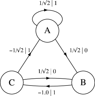
Figure 9: Quantum generator for the Golden Mean Process.

To illustrate that this QDG produces the Golden Mean word distribution we show how to calculate several of the word probabilities using Thm. 10 and Eq. (41):

$$\mathrm{Pr}(0) =n^{-1}\mathrm{dim}(P(0))=\frac{1}{3}~{},$$ (53a)

$$\mathrm{Pr}(1) =n^{-1}\mathrm{dim}(P(1))=\frac{2}{3}~{},$$

$$\mathrm{Pr}(011) =\mathrm{tr}\left(T^{\dagger}(011)\rho^{s}T(011)\right)=\frac{1}{6}.$$ (53b)

VIII.2.2 Quantum Even Process

The next example is a quantum representation of the Even Process. Consider the same spin-$1$ particle. This time the $J_{x}^{2}$ component is chosen as observable. Then $U$ and $P(0)=\mathinner{|{100}\rangle}\mathinner{\langle{100}|}$ and $P(1)=\mathinner{|{011}\rangle}\mathinner{\langle{011}|}$ define a quantum finite-state generator. The QDG is shown in Fig. 10. The word distributions for lengths up to $L=9$ are shown in Fig. 11.

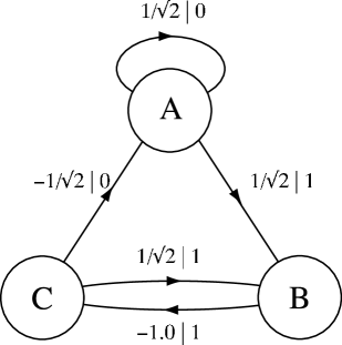
Figure 10: Quantum generator for the Even Process.

Note that the unitary evolution for the Golden Mean Process and the Even Process are the same, just as the state-to-state transition matrices were the same for their classical versions. The partitioning into subspaces induced by the projection operators leads to the (substantial) differences in the word distributions; cf. Figs. 1 versus 11.

The dependence on subspace partitioning indicates a way to count the number of QGs for each unitary evolution $U$. For 3-dimensional Hilbert spaces this is rather straightforward. For each unitary matrix and with a binary alphabet we have three choices for partitioning subspaces of the Hilbert space: one subspace is two-dimensional and the others one-dimensional. This yields three QGs that are distinct up to symbol exchange ($0\leftrightarrow 1$). For the unitary matrix that generates the Golden Mean and the Even Process (Eq. (51)) the third QG turns out to be nondeterministic. But no phase interference is possible and it generates the Golden Mean process language. The potential non-Markovian (sofic) nature of these quantum processes has been discussed in Ref. [15].

This very limited number of possible QGs for any given unitary matrix is yet another indication of the limitations of QGs. Classical SGs do not have the same structural restrictions, since they are not bound by orthogonal partitioning into subspaces, for example. The saving grace for QGs is that they have complex transition amplitudes and so can compute with phase, as long as they are not observed. This is reflected in the distinct languages generated by one QG under different measurement protocols [49].

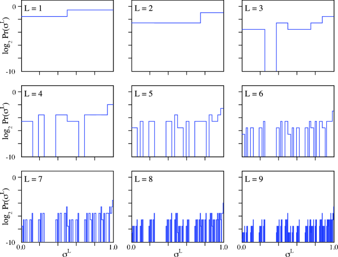
Figure 11: Process language of the Even QDG.

VIII.3 Four-State Quantum Process

We are now in a position to explore the full capabilities of QTs, turning from generators to transducers. The following example illustrates quantum machines by using the tools required to investigate information processing of quantum dynamical systems.

VIII.3.1 Quantum Transducer for Trapped Ions

Consider an atom exposed to short wavelength radiation—the core of numerous experiments that investigate electronic structure and dynamics. The usual procedure is a one-time experiment, exposing the atom to radiation and monitoring changes in structure through electron or photon detectors. As a particular set-up we choose ion-trap experiments found in low-temperature physics and quantum computation implementations, as described in Ref. [7]. For our present purposes it will be sufficient to review the general physical setting.

Imagine a pair of ions kept in a trap by laser fields and static electromagnetic fields. Only two of the electronic levels of each ion are of interest: the ground state and an excited state. Call these level $0$ and level $1$, respectively. A third auxiliary level is required for laser cooling and other operations, which we leave aside here since it has no significance for the description of the process. The two ions are coupled to each other through phonon exchange, as shown schematically in Fig. 12.

By choosing suitable wavelengths several distinct operators can be implemented. One of them is a Hadamard operator that produces a superposition of electronic states $\mathinner{|{0}\rangle}$ and $\mathinner{|{1}\rangle}$. Another is a phase operator that yields an entangled state of the two ions. The respective laser pulses, so-called Rabi pulses, induce an electronic excitation and a vibrational excitation. The result is vibrational coupling of the four levels. All other operations are combinations of these two; see Ref. [7]. The operators are named $U_{a}$, $U_{b}$, and $U_{c}$; matrix representations are given below. As is already familiar from the iterated beam splitter, the operators are activated repeatedly one after the other in a closed loop and as such constitute a quantum dynamical system.

Figure 12: Schematic view of two vibrationally-coupled trapped ions undergoing electronic excitation. Only the two electronic levels of interest are drawn.

To model the quantum dynamical system the state vector and operator matrices need to be specified. The four basis states spanning the Hilbert space are given by:

$$\mathinner{\langle{\phi_{A}}|} =\mathinner{\langle{1000}|},~{}\mathinner{\langle{\phi_{B}}|} =\mathinner{\langle{0100}|},~{}\mathinner{\langle{\phi_{C}}|} =\mathinner{\langle{0010}|},$$

$$\mathinner{\langle{\phi_{D}}|} =\mathinner{\langle{0001}|}.$$

$\phi_{A}$ corresponds to both ions in electronic state $\mathinner{|{0}\rangle}$. $\phi_{B}$ corresponds to ion $1$ in state $\mathinner{|{0}\rangle}$ and ion $2$ in state $\mathinner{|{1}\rangle}$, and so on. The three unitary operations in matrix form are:

$$U_{a} =H\otimes H=\frac{1}{2}\left(\begin{array}[]{rrrr}1&1&1&1\\ 1&-1&1&-1\\ 1&1&-1&-1\\ 1&-1&-1&1\end{array}\right)~{},$$ (54e)

$$U_{b} =\left(\begin{array}[]{rrrr}1&0&0&0\\ 0&1&0&0\\ 0&0&-1&0\\ 0&0&0&-1\end{array}\right)~{},$$ (54j)

$$U_{c} =H\otimes I=\frac{1}{\sqrt{2}}\left(\begin{array}[]{rrrr}1&0&1&0\\ 0&1&0&1\\ 1&0&-1&0\\ 0&1&0&-1\end{array}\right)~{}.$$ (54o)

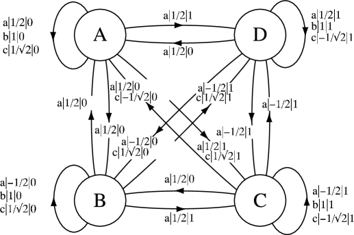
Figure 13: Quantum transducer for a trapped-ion system exposed to radiation of various wavelengths. The input alphabet $X=\{a,b,c\}$ and output alphabet $Y=\{0,1\}$ represent unitary operations and electronic states, respectively.

The projection operators are chosen to measure the electronic state of ion $1$ only and have the matrix form:

$$P(0)=\left(\begin{array}[]{cccc}1&0&0&0\\ 0&1&0&0\\ 0&0&0&0\\ 0&0&0&0\end{array}\right)\mathrm{and}~{}P(1)=\left(\begin{array}[]{cccc}0&0&0&0\\ 0&0&0&0\\ 0&0&1&0\\ 0&0&0&1\end{array}\right).$$ (63)

The QT is now easily assembled. The set of states and the input and output alphabets are, respectively: $Q=\{A,B,C,D\}$, $X=\{a,b,c\}$, and $Y=\{0,1\}$. This QT’s graph is shown in Fig. 13.

To illustrate its operation we consider two measurement protocols. For each we use input sequence $(abc)^{+}$.

• Measurement protocol I: Measure ion $1$ after each unitary operation. The resulting state vector evolution is:

  $$\mathinner{\langle{\psi_{t+1}}|} =\mathinner{\langle{\psi_{t}}|}U_{a}P(y)~{},$$ (64a)

  $$\mathinner{\langle{\psi_{t+2}}|} =\mathinner{\langle{\psi_{t+1}}|}U_{b}P(y)~{},$$ (64b)

  $$\mathinner{\langle{\psi_{t+3}}|} =\mathinner{\langle{\psi_{t+2}}|}U_{c}P(y)~{}.$$ (64c)

• Measurement protocol II: Measure ion $1$ only after three unitary operations. This leads to evolution according to

  $$\mathinner{\langle{\psi_{t+3}}|}=\mathinner{\langle{\psi_{t}}|}U_{a}U_{b}U_{c}P(y)~{}.$$ (65)

The probability distributions of the observed sequences are shown in Figs. 14 and 15. The two distributions differ substantially. On the one hand, protocol II simply yields the process language of alternating $0$s and $1$s. Protocol I, on the other hand, yields a much larger set of allowed words. In particular, it is striking that $\mathrm{supp}\;~{}\mathcal{P}^{\mathrm{II}}$ is forbidden behavior under protocol I. The words $0101$ and $1010$ are forbidden under protocol I, whereas they are the only allowed words of length $L=4$ under protocol II.

Not only does this example illustrate that a simple change in measurement protocol leads to a substantial change in the observed dynamics. It is also not clear a priori when a more complicated behavior is to be expected. That is, more frequent measurement yields more complicated behavior. Without quantifying how complex that complicated behavior is, it turns out that it is not always the longer period of coherent, unperturbed unitary evolution that yields more complex processes. This will have consequences for feasible implementations of quantum computational algorithms. For a quantitative discussion of the languages generated by quantum processes see Ref. [21].

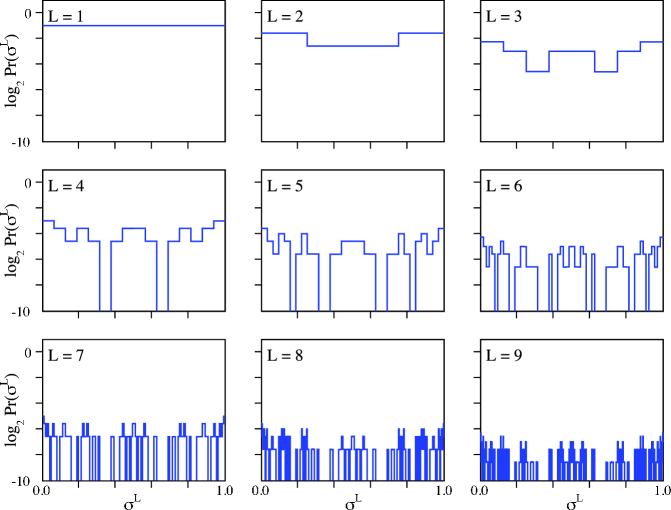
Figure 14: Process language generated by the trapped-ion quantum dynamical system of Fig. 12 for protocol I (measurements performed at each time step).

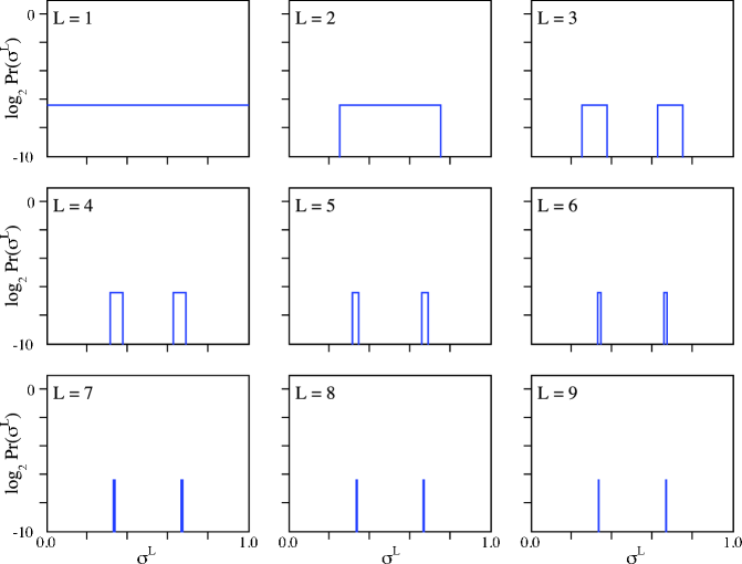
Figure 15: The generated process languages of the trapped-ion dynamical system from Fig. 12 for measurements performed every three time steps.

VIII.3.2 Deutsch Algorithm as a Special Case

It turns out that the trapped-ion experiment implements a quantum algorithm first introduced by Deutsch [6]. The algorithm provided an explicit example of how a quantum machine could be superior to a classical one.

Consider a binary-valued function $f:\{1,2,\dots,2N\}\rightarrow\{0,1\}$. Let $U$ be the device that computes the function $f$. If we successively apply $f$ to $1,2,\dots,2N$, we get a string $x^{2N}$ of length $2N$. The problem then is to find a true statement about $x^{2N}$ by testing the following two properties:

• $f$ is not constant: Not only $0$s or only $1$s in $x^{2N}$.

• $f$ is not balanced: Not as many $0$s as $1$s in $x^{2N}$.

If statement A is false, we can be certain that statement B is true and vice versa. Note that both statements can be true in which case the algorithm does not reveal anything about $f$. Deutsch and Josza [50] showed that a quantum computer can determine the true statement, either A or B, after only two invocations of the operation $U$, whereas a classical computer requires $N+1$ calls in the worst case. Taking into account the computational steps for establishing the start state and reading out the result, a quantum computer can evaluate the function $f$ in constant time, whereas a classical computer needs a time linear in $N$.

To compare the algorithm with the trapped-ion dynamical system, and to keep issues simple but still informative, we use the basic version ($N=2$) of the Deutsch algorithm of Ref. [47, p. 32]. (Recall that in our notation $\mathinner{\langle{\psi}|}$ is the state vector, not $\mathinner{|{\psi}\rangle}$, as is common elsewhere.) Figure 16 shows the algorithm as a quantum circuit. Each qubit represents one ion and occupies one horizontal line. The applied unitary transformations are shown as boxes. The overall procedure is summarized in Table 1. The unitary operations $H$ and $U_{f}$ in Fig. 16 are the same as $H$ and $U_{b}$ in the trapped-ion experiment. The unitary operator is that for a balanced function.

The implementation of the Deutsch algorithm is equivalent to the trapped-ion system under measurement protocol II, with $U_{b}$ chosen accordingly. Measuring ion $1$ after three time steps delivers the desired answer as output ($0$=A or $1$=B). Thus, the Deutsch algorithm corresponds to the trapped-ion system running for three time steps.

The Deutsch algorithm task is solved with a considerable speed-up compared to a classical implementation. Our approach is an extension of this that focuses on what type of computation is carried out intrinsically by the system under continuous external driving and observation. The answer is found in the language diagrams in Figs. 14 and 15. Comparing these two different views of quantum information manipulation—designed quantum computing versus quantum intrinsic computation—suggests that the analysis of NMR experiments with single atoms or molecules in terms of quantum finite-state machines will be a straightforward extensions of the preceding analysis of the Deutsch algorithm.

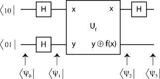
Figure 16: Deutsch algorithm to classify balanced and constant functions ($N=2$) depicted as a quantum circuit.

1. Two qubits put in states	$\mathinner{\langle{\psi^{0}}|}=\mathinner{\langle{0100}|}$
$~{}~{}~{}~{}\mathinner{\langle{0}|}$ and $\mathinner{\langle{1}|}$, respectively.
2. Hadamard transform applied	$\mathinner{\langle{\psi_{1}}|}=\mathinner{\langle{\psi^{0}}|}(H\otimes H)$
to both qubits.
3. Operation $U_{f}$ implementing	$\mathinner{\langle{\psi_{2}}|}=(-1)^{f(x)}\mathinner{\langle{\psi_{1}}|}(I\otimes I)$
the function $f(x)$ is applied.
4. Hadamard transform applied	$\mathinner{\langle{\psi_{3}}|}=\mathinner{\langle{\psi_{2}}|}(H\otimes I)$
to the first qubit.
5. First qubit is measured.	$\mathinner{\langle{\psi_{3}}|}P(0)$

Table 1: Deutsch algorithm to determine if $f(x)$ is balanced or constant. $H$ and $I$ are the Hadamard and identity matrices, respectively. $\otimes$ denotes the tensor product.

IX Concluding Remarks

We developed a line of inquiry complementary to both quantum computation and quantum dynamical systems by investigating intrinsic computation in quantum processes. Laying the foundations for a computational perspective on quantum dynamical systems, we introduced quantum finite-state transducers. Residing at the lowest level of a quantum computational hierarchy, it is the most general representation of a finitary quantum process. It allows for a quantitative description of intrinsic computation in quantum processes—in terms of the number of internal states and allowed transitions and the process language it generates. As far as we are aware, this has not been developed before in the quantum setting.

We laid out the mathematical foundations of these models and developed a hierarchy of classical (stochastic) and quantum machines in terms of the set of process languages they recognize or generate. In many cases it turned out that quantum devices were less powerful than their classical analogs. We saw that the limitations of quantum finite-state machines originate in the unitarity of the transition matrices. This suggested that QTs, being reversible, are less powerful than nonreversible classical automata, since the reversibility constrains the transition matrices.

However, one must be careful to not over-interpret this state of affairs. It has been known for some time that any universal computation can be implemented in a reversible device [51]. Typically, this requires substantially more resources, largely to store outcomes of intermediate steps. In short, reversibility does not, in general, imply less power for classical computers. At the end of the day, computational resources are variables that trade-off against each other. The 2-state QDG examples of the Beam Splitter process illustrated such a trade-off. Although the QDG needs more states than the equivalent SDG to generate the same process language, different measurement protocols yielded a new set of process languages—an aspect that makes QDGs more powerful than SDGs [49].

These results were then applied to physical systems that could be analyzed in terms of the process languages they generate. One example, that of two trapped ions exhibited a process language with rich structure. This, and the fact that the system implements a quantum algorithm, opens up a way to an information-theoretic analysis of quantum processes. One can begin to analyze quantum algorithms in terms of their information processing power and do so independent of particular physical implementations.

In particular, we have used quantum machines to define a measure of intrinsic computation for quantum dynamical systems [21, 15]. The basic questions one asks about a dynamical system’s intrinsic computation—amount of historical information stored, storage architecture, and transformations of stored information—can now be posed for quantum systems.

Furthermore, we are developing an extension of quantum machines that supports more general types of measurement. The resulting quantum transducers are expected to have greater power than the current versions, possibly even greater than stochastic transducers. Generally, we hope that ways to integrate quantum computation and quantum dynamics will receive further attention.

- [1] W. McCulloch and W. Pitts. A logical calculus of ideas immanent in nervous activity. Bulletin of Mathematical Biophysics, 5:115–133, 1943.
- [2] M. A. Arbib, editor. The Handbook of Brain Theory and Neural Networks. MIT Press, 2002.
- [3] N. Chomsky. Three models for the description of language. IRE Trans. Info. Th., 2:113, 1956.
- [4] P. Shor. Polynomial-time algorithms for prime factorization and discrete logarithms on a quantum computer. In Proceedings of the 35th Annual Symposium on Foundations of Computer Science, page 124, 1994.
- [5] L. K. Grover. A fast quantum mechanical algorithm for database search. In 28th Annual ACM Symposium on the Theory of Computation, page 212, 1996.
- [6] D. Deutsch. Quantum theory, the Church-Turing principle and the universal quantum computer. Proc. Roy. Soc. London A, 400:97, 1985.
- [7] A Galindo and M. A. Martín-Delgado. Information and computation: Classical and quantum aspects. Rev. Mod. Phys., 74:347–423, 2002.
- [8] P. Zoller et al. Quantum information processing and communication. Eur. Phys. J. D, 36:203–228, 2005.
- [9] E. Knill, R. Laflamme, R. Martinez, and C.-H. Tseng. An algorithmic benchmark for quantum information processing. Nature, 404:368–370, 2000.
- [10] R. Alicki and M. Fannes. Quantum Dynamical Systems. Oxford University Press, 2001.
- [11] B. Kümmerer. Quantum Markov processes. In Lecture Notes in Physics, pages 139–198. Springer, 2002.
- [12] M. C. Gutzwiller. Chaos in Classical and Quantum Mechanics. Springer Verlag, 1990.
- [13] S. Habib, K. Jacobs, and K. Shizume. Emergence of chaos in quantum systems far from the classical limit. Phys. Rev. Lett., 96:010403–06, 2006.
- [14] D. Lind and B. Marcus. An Introduction to Symbolic Dynamics and Coding. Cambridge University Press, 1995.
- [15] K. Wiesner and J. P. Crutchfield. Computation in sofic quantum dynamical systems. In S.G. Akl, C. S. Calude, M. J. Dinneen, G. Rozenberg, and H. T. Wareham, editors, Unconventional Computation, Proceedings of the Sixth International Conference UC’07, (Kingston, Canada, 13-17 August 2007), volume 4618 of Lect. Notes Comp. Sci., Berlin, 2007. Springer.
- [16] J. P. Crutchfield. The calculi of emergence: Computation, dynamics, and induction. Physica D, 75:11–54, 1994.
- [17] J. P. Crutchfield and K. Young. Inferring statistical complexity. Phys. Rev. Let., 63:105–108, 1989.
- [18] J. P. Crutchfield and K. Young. Computation at the onset of chaos. Entropy, Complexity and the Physics of Information, SFI Studies in the Sciences of Complexity, VIII:223–269, 1990.
- [19] J. P. Crutchfield and J. E. Hanson. Turbulent pattern basis for cellular automata. Physica D, 69:279–301, 1993.
- [20] J. P. Crutchfield and D. P. Feldman. Statistical complexity of simple 1d spin systems. Phys. Rev. E, 55:1239–1243, 1997.
- [21] J. P. Crutchfield and K. Wiesner. Intrinsic quantum computation. Physics Letters A, 372:375–380, 2007.
- [22] B. Weiss. Subshifts of finite type and sofic systems. Monatsh. Math., 77:462, 1973.
- [23] W. Bialek, I. Nemenman, and N. Tishby. Predictability, complexity, and learning. Neural Comp., 13:2409–2463, 2001.
- [24] P. Vitányi. Meaningful information. Lect. Notes Comp. Sci., 2518:53–62, 2002.
- [25] J. P. Crutchfield and D. P. Feldman. Regularities unseen, randomness observed: Levels of entropy convergence. Chaos, 13:25 – 54, 2003.
- [26] A. Paz. Introduction to Probabilistic Automata. New York Academic Press, 1971.
- [27] M. O. Rabin. Probabilistic automata. Information and Control, 6:230–245, 1963.
- [28] E. Vidal, F. Thollard, C. de la Higuera, F. Casacuberta, and R. C. Carrasco. Probabilistic finite-state machines–Part I. IEEE Trans. Patt. Anal. Mach. Intel., 27:1013–1025, 2005.
- [29] J. E. Hopcroft, R. Motwani, and J. D. Ullman. Introduction to Automata Theory, Languages, and Computation. Addison-Wesley, 2001.
- [30] W. Thomas. Automata on infinite objects. In Van Leeuwen, editor, Handbook of Theoretical Computer Science, pages 133–164. Elsevier, Amsterdam, 1990.
- [31] P. Grassberger. Toward a quantitative theory of self-generated complexity. Intl. J. Theo. Phys., 25:907, 1986.
- [32] A. Fraser. Chaotic data and model building. In H. Atmanspacher and H. Scheingraber, editors, Information Dynamics, volume Series B: Physics Vol. 256 of NATO ASI Series, page 125, New York, 1991. Plenum.
- [33] D. Auerbach and I. Procaccia. Grammatical complexity of strange sets. Phys. Rev. A, 41:6602–6614, 1990.
- [34] W. Yi and H.Xie. Grammatical complexity of unimodal maps with eventually periodic kneading sequences. Nonlinearity, 7:1419–1436, 1994.
- [35] R. Shankar. Principles of Quantum Mechanics. Plenum Press, New York, 1994.
- [36] C. Cohen-Tannoudji, B. Diu, and F. Laloe. Quantum Mechanics. John Wiley & Sons, Singapore, 2005.
- [37] S. Gudder. Quantum automata: An overview. International Journal of Theoretical Physics, 38:2261–2272, 1999.
- [38] R. Freivalds and A. Winter. Quantum finite state transducers. Lect. Notes Comp. Sci., 2234:233–242, 2001.
- [39] S. Severini. On the digraph of a unitary matrix. SIAM J. Matrix Anal. Appl., 25:295–300, 2003.
- [40] D. Z. Albert. On quantum-mechanical automata. Physics Letters A, 98:249–251, 1983.
- [41] A. Peres. On quantum-mechanical automata. Physics Letters A, 101:249–250, 1984.
- [42] A. Kondacs and J. Watrous. On the power of quantum finite state automata. In 38th IEEE Conference on Foundations of Computer Science, pages 66–75, 1997.
- [43] D. Aharonov, A. Kitaev, and N. Nisan. Quantum circuits with mixed states. Symp. Th. Comp. (STOC 1998), pages 20–30, 1998.
- [44] A. Bertoni and M. Carpentieri. Analogies and differences between quantum and stochastic automata. Theor. Comp. Sci., 262:69–81, 2001.
- [45] C. Moore and J. P. Crutchfield. Quantum automata and quantum grammars. Theor. Comp. Sci., 237:275–306, 2000.
- [46] T. Cover and J. Thomas. Elements of Information Theory. Wiley-Interscience, 1991.
- [47] M. A. Nielsen and I. L. Chuang. Quantum computation and quantum information. Cambridge University Press, 2000.
- [48] A. Peres. Quantum Theory: Concepts and Methods. Kluwer Academic Publishers, 1993.
- [49] K. Wiesner and J. P. Crutchfield. Language diversity of measured quantum processes. Intl. J. Unconventional Computing, 4(1):99–112, 2008.
- [50] D. Deutsch and R. Josza. Rapid solution of problems by quantum computation. Proc. Roy. Soc. London A, 439:553–558, 1992.
- [51] C. H. Bennett. Logical reversibility of computation. IBM J. Res. Dev., 17(6):525–532, 1973.