Visualization of superposition of macroscopically distinct states

Abstract

We propose a method of visualizing superpositions of macroscopically distinct states in many-body pure states. We introduce a visualization function, which is a coarse-grained quasi joint probability density for two or more hermitian additive operators. If a state contains superpositions of macroscopically distinct states, one can visualize them by plotting the visualization function for appropriately taken operators. We also explain how to efficiently find appropriate operators for a given state. As examples, we visualize four states containing superpositions of macroscopically distinct states: the ground state of the XY model, that of the Heisenberg antiferromagnet, a state in Shor’s factoring algorithm, and a state in Grover’s quantum search algorithm. Although the visualization function can take negative values, it becomes non-negative (hence becomes a coarse-grained joint probability density) if the characteristic width of the coarse-graining function used in the visualization function is sufficiently large.

I introduction

Visualization functions, such as the Wigner distribution function Wigner and the Husimi function husimi , are very useful. By plotting them, one can visualize quantum states to understand structure of these states. Furthermore, because these functions are, in some senses, probability densities, one can interpret various experimental results by using these functions Mandel . Although there are many methods of visualizing quantum states with small degrees of freedom Mandel , those of visualizing quantum many-body states are very few  Wooters ; Leonhardt ; Hannay ; Rivas . It is therefore important to develop methods of visualizing quantum many-body states.

In quantum many-body systems, which include quantum computers Nielsen ; Grover ; Shor ; Ekert , there are many states which contain superpositions of macroscopically distinct states Schrodinger ; Leggett1 ; Nakamura ; Friedman ; Wal ; Mermin ; Wakita ; Grib ; Cirac ; SM ; Morimae ; SM05 ; Ukena ; Ukena2 ; Boson . Existence of a superposition of macroscopically distinct states in a many-body pure state can be identified by an index $p$ $(1\leq p\leq 2)$ SM ; Sugita ; Morimae ; Ukena ; Ukena2 : If a given pure state has $p=2$, it contains a superposition of macroscopically distinct states SM ; Morimae .

If every macroscopic superposition could be reduced to an equal-weight superposition of two macroscopically distinct states, such as $\frac{1}{\sqrt{2}}|0\cdots 0\rangle+\frac{1}{\sqrt{2}}|1\cdots 1\rangle$, visualization of macroscopic superpositions would be a trivial task. However, there are many other states in which many macroscopically distinct states are superposed with various weights SM ; Morimae ; SM05 ; Ukena ; Ukena2 ; Boson . Therefore it is also important to develop good methods of visualizing such complicated superpositions.

In this paper, we propose a method of visualizing superpositions of macroscopically distinct states contained in states having $p=2$. We first introduce a function $\Xi(A_{1},\cdots,A_{m})$, which is interpreted as a coarse-grained quasi joint probability density for hermitian additive operators $\hat{A}_{1},\cdots,\hat{A}_{m}$. We next explain how to find appropriate $\hat{A}_{1},\cdots,\hat{A}_{m}$ efficiently for a given pure state. One can visualize superpositions of macroscopically distinct states contained in a given pure state having $p=2$ by plotting $\Xi(A_{1},\cdots,A_{m})$ for appropriate $\hat{A}_{1},\cdots,\hat{A}_{m}$. As examples, we visualize four states having $p=2$: the ground state of the XY model, that of the Heisenberg antiferromagnet, a state in Shor’s factoring algorithm Shor , and a state in Grover’s quantum search algorithm Grover . Although $\Xi$ can take negative values, like the Wigner distribution function, it becomes non-negative, hence becomes a coarse-grained joint probability density, if the characteristic width of the coarse-graining function used in $\Xi$ is sufficiently large.

This paper is organized as follows. After briefly reviewing the index $p$ in the next section, we introduce $\Xi$ in Sec. III.1, and explain how to find appropriate operators efficiently in Sec. III.2. We visualize four states in Sec. IV. Discussion is given in Sec. V.

II Index $p$

To establish notation, and for the convenience of the reader, we briefly review the index $p$ in this section. For details, see Refs. SM ; Ukena ; Ukena2 ; Sugita ; Morimae ; SM05 .

We first fix the energy range of interest. It determines the degrees of freedom of an effective theory which describes the system under consideration. We assume that the system is, in that energy range, described as an $N$-site lattice. Throughout this paper, we assume that $N$ is large but finite.

For simplicity, we here consider only pure states, although the definition of superposition of macroscopically distinct states has been successfully generalized to mixed states SM05 . Furthermore, we assume that states are spatially homogeneous, or effectively homogeneous as in quantum chaotic systems Sugita or in quantum computers Ukena ; Ukena2 . For such states, we can consider a family of similar states $\{|\psi^{N}\rangle\}_{N}$. For example, each member of the family $\{|E_{0}^{N}\rangle\}_{N}$ of the ground states of the XY model is the ground state $|E_{0}^{N}\rangle$ of the XY Hamiltonian of an $N$-site system.

The index $p$ is defined for such families of similar states. For simplicity, we represent a family of states $\{|\psi^{N}\rangle\}_{N}$ by a representative state $|\psi\rangle$ $(=|\psi^{N}\rangle)$. The index $p$ $(1\leq p\leq 2)$ of $|\psi\rangle$ is then defined by

$$\max_{\hat{A}}\langle\psi|(\Delta\hat{A})^{2}|\psi\rangle=\mathcal{O}(N^{p}),$$ (1)

where $\Delta\hat{A}\equiv\hat{A}-\langle\psi|\hat{A}|\psi\rangle$ O , and the maximum is taken over all hermitian additive operators $\hat{A}$. Here, an additive operator $\hat{A}$ is a sum of local operators: $\hat{A}=\sum_{l=1}^{N}\hat{a}(l)$, where $\hat{a}(l)$ is a local operator, which is independent of $N$, on site $l$. We do not assume that $\hat{a}(l^{\prime})$ ($l^{\prime}\neq l$) is the spatial translation of $\hat{a}(l)$.

If $p=2$, there is a hermitian additive operator which ‘fluctuates macroscopically’ in the sense that the relative fluctuation does not vanish in the limit of $N\to\infty$:

$$\frac{\sqrt{\langle\psi|(\Delta\hat{A})^{2}|\psi\rangle}}{N}\nrightarrow 0\ \ (N\to\infty).$$ (2)

Because $|\psi\rangle$ is pure, the reason for the macroscopic fluctuation is that eigenstates of $\hat{A}$ corresponding to macroscopically distinct eigenvalues are superposed with sufficiently large weights in $|\psi\rangle$. Here, two eigenvalues $A$ and $A^{\prime}$ are macroscopically distinct if and only if $A-A^{\prime}=\mathcal{O}(N)$. Therefore a pure state having $p=2$ contains a superposition of macroscopically distinct states (see Refs. Morimae ; SM05 for detailed discussion). On the other hand, if $p<2$, all additive operators ‘have macroscopically definite values’ in the sense that relative fluctuations of all additive operators vanish as $N\to\infty$. In this case, there is no superposition of macroscopically distinct states in $|\psi\rangle$. In short, one can judge whether a pure state contains a superposition of macroscopically distinct states or not by calculating the index $p$.

There is an efficient method of calculating $p$. For simplicity, we henceforth assume that each site of the lattice is a spin-$1/2$ system. For a given pure state $|\psi\rangle$, we define the variance-covariance matrix (VCM) by

$$V_{\alpha l,\beta l^{\prime}}\equiv\langle\psi|\Delta\hat{\sigma}_{\alpha}(l)\Delta\hat{\sigma}_{\beta}(l^{\prime})|\psi\rangle,$$ (3)

where $\alpha,\beta=x,y,z$; $l,l^{\prime}=1,2,\cdots,N$; $\hat{\sigma}_{x}(l)$, $\hat{\sigma}_{y}(l)$, and $\hat{\sigma}_{z}(l)$ are Pauli operators on site $l$. The VCM is a $3N\times 3N$ hermitian non-negative matrix. If $e_{1}$ is the maximum eigenvalue of the VCM, then $e_{1}=\mathcal{O}(N^{p-1})$, as shown in Appendix A. One therefore has only to evaluate $e_{1}$ to calculate $p$.

III Visualization method

By calculating the index $p$, one can judge whether a pure state contains a superposition of macroscopically distinct states or not. From $p$ only, however, one cannot know detailed structures of the superposition of macroscopically distinct states, including which macroscopically distinct states are superposed and with what weights they are superposed. In this section, we propose a method of visualizing these structures of superpositions of macroscopically distinct states.

III.1 Visualization function $\Xi$

Let $\hat{A}=\sum_{l}\hat{a}(l)$ and $\hat{B}=\sum_{l}\hat{b}(l)$ be hermitian additive operators. We assume that $[\hat{A},\hat{B}]\neq 0$, so that the joint probability distribution for $\hat{A}$ and $\hat{B}$ does not exist in general.

For macroscopic systems, one is usually interested in states in which typical values of additive operators are $\mathcal{O}(N)$ O . Typical values of $\hat{A}/N$ and $\hat{B}/N$ are therefore $\mathcal{O}(N^{0})$. Their commutator is small in the sense that

$$\left\|\left[\frac{\hat{A}}{N}~{},~{}\frac{\hat{B}}{N}\right]\right\|=O\left(\frac{1}{N}\right),$$ (4)

because $[\hat{a}(l),\hat{b}(l^{\prime})]=0$ for $l\neq l^{\prime}$ O ; SM05 ; Grib . Since $N$ is large but finite, the above commutator does not vanish. In real experiments, however, resolutions of measurements are limited. Equation (4) therefore indicates that noncommutativity of additive operators could not be detected for large $N$. This suggests that we may be able to introduce a function which can be well regarded as a coarse-grained joint probability density for $\hat{A}$ and $\hat{B}$. Note that the finite resolution is essential, because noncommutativity, however small it is, can be detected if the resolutions of experiments are high enough xp .

We formulate the above idea as follows. Consider the spectral decompositions of $\hat{A}$ and $\hat{B}$:

$$\hat{A}=\sum_{A\in\mathbb{E}_{\hat{A}}}A\mathcal{P}_{\hat{A}}(A),\ \hat{B}=\sum_{B\in\mathbb{E}_{\hat{B}}}B\mathcal{P}_{\hat{B}}(B),$$ (5)

where $\mathbb{E}_{\hat{A}}$ and $\mathbb{E}_{\hat{B}}$ are the spectra of $\hat{A}$ and $\hat{B}$, respectively, and $\mathcal{P}_{\hat{A}}(A)$ and $\mathcal{P}_{\hat{B}}(B)$ are the projection operators onto the eigenspaces of eigenvalues $A$ and $B$, respectively. To take account of finite resolutions of experiments, we smear the projection operators to obtain

$$\overline{\mathcal{P}}_{\hat{A}}(A)\equiv\sum_{A^{\prime}\in\mathbb{E}_{\hat{A}}}w_{\hat{A}}(A,A^{\prime})\mathcal{P}_{\hat{A}}(A^{\prime}),$$ (6)

and similarly for $\overline{\mathcal{P}}_{\hat{B}}(B)$. Here, $A$ is a real continuous variable ($A\in\mathbb{R}$), and $w_{\hat{A}}(A,A^{\prime})$ is a coarse-graining function. It centers at $A=A^{\prime}$ with a characteristic width $W_{\hat{A}}$, and satisfies

$$w_{\hat{A}}(A,A^{\prime})\geq 0\quad\mbox{for all }A,A^{\prime},$$ (7)

$$\int_{-\infty}^{+\infty}w_{\hat{A}}(A,A^{\prime})dA=1\quad\mbox{for all }A^{\prime}.$$ (8)

The coarse-graining functions $w_{\hat{A}},w_{\hat{B}}$ should not have complicated forms; they should be physically reasonable ones. To be definite, we henceforth assume that $W_{\hat{A}}=W_{\hat{B}}=W$ and $w_{\hat{A}}(X,X^{\prime})=w_{\hat{B}}(X,X^{\prime})=w(X-X^{\prime})$, where

$$w(X)={1\over\sqrt{2\pi}W}\exp\left(-{X^{2}\over 2W^{2}}\right).$$ (9)

Clearly, $\overline{\mathcal{P}}_{\hat{A}}(A)$ and $\overline{\mathcal{P}}_{\hat{B}}(B)$ are non-negative hermitian operators satisfying

$$\int_{-\infty}^{+\infty}\overline{\mathcal{P}}_{\hat{A}}(A)dA=\int_{-\infty}^{+\infty}\overline{\mathcal{P}}_{\hat{B}}(B)dB=\hat{1}.$$ (10)

They give coarse-grained probability densities $\Xi_{\hat{A}}$ and $\Xi_{\hat{B}}$ for $\hat{A}$ and $\hat{B}$, respectively, for a given pure state $|\psi\rangle$ by

$$\Xi_{\hat{A}}(A)=\langle\psi|\overline{\mathcal{P}}_{\hat{A}}(A)|\psi\rangle\quad(A\in\mathbb{R}),$$ (11)

$$\Xi_{\hat{B}}(B)=\langle\psi|\overline{\mathcal{P}}_{\hat{B}}(B)|\psi\rangle\quad(B\in\mathbb{R}).$$ (12)

Now we define

$$\Xi(A,B)\equiv\frac{1}{2}\langle\psi|\overline{\mathcal{P}}_{\hat{A}}(A)\overline{\mathcal{P}}_{\hat{B}}(B)+\overline{\mathcal{P}}_{\hat{B}}(B)\overline{\mathcal{P}}_{\hat{A}}(A)|\psi\rangle$$ (13)

for $A,B\in\mathbb{R}$. One can easily verify the following:

$$\Xi(A,B)\mbox{ is real},$$ (14)

$$\int\int_{-\infty}^{+\infty}\Xi(A,B)dAdB=1,$$ (15)

$$\int_{-\infty}^{+\infty}\Xi(A,B)dB=\Xi_{\hat{A}}(A),\ \int_{-\infty}^{+\infty}\Xi(A,B)dA=\Xi_{\hat{B}}(B).$$ (16)

In general, $\Xi(A,B)$ can take negative values. If it is non-negative, Eqs. (15) and (16) show that it can be interpreted as a coarse-grained joint probability density (cgJPD) for $\hat{A}$ and $\hat{B}$. In fact, as we will demonstrate in the following sections, $\Xi(A,B)$ becomes non-negative if $W$ and $N$ are large enough, for many states of interest. Furthermore, even if $W$ and $N$ are not large, negative-valued regions of $\Xi(A,B)$ are small. In this case, $\Xi(A,B)$ can be considered as a coarse-grained quasi joint probability density (cgQJPD) for $\hat{A}$ and $\hat{B}$.

The non-negativity of $\Xi(A,B)$ becomes obvious as $W\to\infty$, for which $\Xi(A,B)\sim w(A)w(B)\geq 0$ for all $A,B$. For smaller $W$, the smallest value of $W$ that makes $\Xi(A,B)$ non-negative depends on $\hat{A}$, $\hat{B}$ and $|\psi\rangle$. Therefore, in general, the non-negativity should be checked a posteriori.

We can also introduce $\Xi$ for $m$ ($\geq 3$) hermitian additive operators $\hat{A}_{1},\hat{A}_{2},\cdots,\hat{A}_{m}$ by

$$\Xi(A_{1},\cdots,A_{m})$$

$$\equiv\frac{1}{m!}\sum_{\pi}\langle\psi|\overline{\mathcal{P}}_{\hat{A}_{\pi(1)}}(A_{\pi(1)})\cdots\overline{\mathcal{P}}_{\hat{A}_{\pi(m)}}(A_{\pi(m)})|\psi\rangle,$$ (17)

where the sum is taken over all permutations $\pi$ of the numbers $1,2,\cdots,m$.

If $|\psi\rangle$ has $p=2$, one can visualize structure of the macroscopic superpositions contained in $|\psi\rangle$ by plotting $\Xi(A_{1},\cdots,A_{m})$ versus $(A_{1},\cdots,A_{m})$, if $\hat{A}_{1},\cdots,\hat{A}_{m}$ are appropriately taken. We call such a plot a visualization of superpositions of macroscopically distinct states in $|\psi\rangle$. An efficient method of finding appropriate $\hat{A}_{1},\cdots,\hat{A}_{m}$ will be explained in the next subsection.

III.2 Efficient method of finding appropriate operators

In principle, one can take any hermitian additive operators $\hat{A}_{1},\cdots,\hat{A}_{m}$, and plot $\Xi(A_{1},\cdots,A_{m})$. In this paper, however, we are interested in states having $p=2$, which contain superpositions of macroscopically distinct states. Such superpositions are characterized by macroscopic fluctuations of certain additive operators (see Sec. II and Refs. SM ; Morimae ). Therefore, as will be demonstrated in the next section, we can visualize such superpositions by including macroscopically fluctuating operator(s) in $\hat{A}_{1},\cdots,\hat{A}_{m}$ of $\Xi(A_{1},\cdots,A_{m})$. In this subsection, we present an efficient method of finding a set $\mathcal{S}$ of macroscopically fluctuating hermitian additive operators.

For a given pure state $|\psi\rangle$, we diagonalize the VCM to obtain its eigenvalues, $e_{1}\geq e_{2}\geq\cdots\geq e_{3N}$, and eigenvectors. From the eigenvectors, we construct a complete orthogonal system: $\{\{\tilde{c}_{\alpha l}^{~{}1}\},\{\tilde{c}_{\alpha l}^{~{}2}\},\cdots,\{\tilde{c}_{\alpha l}^{~{}3N}\}\}$ ($\alpha=x,y,z$; $l=1,2,\cdots,N$). Here, $\{\tilde{c}_{\alpha l}^{~{}i}\}\in\mathbb{C}^{3N}$ is an eigenvector of the VCM corresponding to $e_{i}$. We assume that each $\tilde{c}_{\alpha l}^{~{}i}$ is asymptotically independent of $N$, and that we can normalize $\{\tilde{c}_{\alpha l}^{~{}i}\}$ as $\sum_{\alpha l}|\tilde{c}_{\alpha l}^{~{}i}|^{2}=N$. By taking an appropriate limit of $\{\tilde{c}_{\alpha l}^{~{}i}\}$ as described in Appendix B, we obtain a vector $\{c_{\alpha l}^{i}\}$, whose elements are independent of $N$. From this vector, we construct the additive operator:

$$\hat{A}_{i}\equiv\sum_{l=1}^{N}\sum_{\alpha=x,y,z}c_{\alpha l}^{i}\hat{\sigma}_{\alpha}(l).$$ (18)

As shown in Appendix C, $\hat{A}_{i}$ fluctuates macroscopically if and only if $e_{i}=\mathcal{O}(N)$.

If $e_{i}=\mathcal{O}(N)$ and $\hat{A}_{i}$ is hermitian, we let $\hat{A}_{i}$ be an element of $\mathcal{S}$. If $e_{i}=\mathcal{O}(N)$ and $\hat{A}_{i}$ is non-hermitian, on the other hand, we decompose $\hat{A}_{i}$ into the real and the imaginary parts: $\hat{A}_{i}=\hat{A}_{i}^{\rm re}+i\hat{A}_{i}^{\rm im}$, where $\hat{A}_{i}^{\rm re}\equiv(\hat{A}_{i}+\hat{A}_{i}^{\dagger})/2$ and $\hat{A}_{i}^{\rm im}\equiv(\hat{A}_{i}-\hat{A}_{i}^{\dagger})/2i$. It is known that $\hat{A}_{i}^{\rm re}$ and/or $\hat{A}_{i}^{\rm im}$ fluctuate(s) macroscopically (see Ref. Morimae and Appendix A). We let such macroscopically fluctuating part(s) be an element(s) of $\mathcal{S}$. In this way, we obtain a set of macroscopically fluctuating hermitian additive operators, e.g., as $\mathcal{S}=\{\hat{A}_{1},\hat{A}_{2}^{\rm im},\hat{A}_{3},\hat{A}_{4}^{\rm re},\hat{A}_{4}^{\rm im},\hat{A}_{5}\}$. Several examples of $\mathcal{S}$ will be given in the next section. Any macroscopically fluctuating additive operator includes at least one element of $\mathcal{S}$ as a component in the sense explained in Appendix D.

The number of the elements of $\mathcal{S}$ is $O(N^{0})$, because $e_{i}\geq 0$ and $\sum_{i=1}^{3N}e_{i}=\sum_{l=1}^{N}\sum_{\alpha=x,y,z}V_{\alpha l,\alpha l}\leq 3N$. One can obtain $\mathcal{S}$ efficiently, because one has only to diagonalize the VCM, which is a $3N\times 3N$ hermitian matrix.

By including an element(s) of $\mathcal{S}$ into $\hat{A}_{1},\cdots,\hat{A}_{m}$ of $\Xi(A_{1},\cdots,A_{m})$, one can visualize superpositions of macroscopically distinct states in $|\psi\rangle$ by plotting $\Xi(A_{1},\cdots,A_{m})$.

IV Examples

To demonstrate usefulness of the visualization method, we visualize four states having $p=2$ in this section.

IV.1 XY model

First, we visualize the exact ground state of the XY model on a two-dimensional square lattice of $N$ sites. The Hamiltonian is

$$\hat{H}=-\sum_{<l,l^{\prime}>}\left[\hat{\sigma}_{x}(l)\hat{\sigma}_{x}(l^{\prime})+\hat{\sigma}_{y}(l)\hat{\sigma}_{y}(l^{\prime})\right],$$ (19)

where $<l,l^{\prime}>$ denotes the nearest neighbors. If $N$ is finite, ‘ground states’ obtained by the mean-field approximation are very different from the exact ground state SMU(1) ; Koma ; Oitmaa ; Miyashita ; Yukalov . These mean-field ground states are degenerate symmetry-breaking states with non-zero order parameters. They are separable states, because the mean-field approximation neglects the correlations between sites. On the other hand, the exact ground state is unique, symmetric, and has $p=2$ SMU(1) ; Koma ; Oitmaa ; Miyashita ; Morimae . We visualize the exact ground state.

By numerical calculations, we find that $e_{1}=e_{2}=\mathcal{O}(N)$, $e_{i}=o(N)$ $(i\geq 3)$, $\hat{A}_{1}=\sum_{l=1}^{N}\hat{\sigma}_{x}(l)\equiv\hat{M}_{x}$, and $\hat{A}_{2}=\sum_{l=1}^{N}\hat{\sigma}_{y}(l)\equiv\hat{M}_{y}$. Hence,

$${\mathcal{S}}=\{\hat{M}_{x},\hat{M}_{y}\}.$$ (20)

In Fig. 1, we plot $\Xi(M_{x},M_{y})$ for $N=14$ without coarse-graining, i.e., $W\to 0$, for which the coarse-graining function of Eq. (9) becomes the delta function $\delta(X)$. In the figure, $c\delta(0)$ [$c\in\mathbb{R}$] is represented by a vertical line with height $c$. Positive values are represented by red vertical lines, whereas negative values are represented by blue vertical lines. Because $\Xi(M_{x},M_{y})$ takes negative values at some points, it is not a JPD for $\hat{M}_{x}$ and $\hat{M}_{y}$.

However, negative values are expected to approach 0 as $W$ is increased. To see this, we plot in Fig. 2 the integral $I_{\hat{M}_{x},\hat{M}_{y}}$ of negative values versus $W$, where $I_{\hat{A},\hat{B}}$ is defined by

$$I_{\hat{A},\hat{B}}\equiv\int\int_{-\infty}^{+\infty}dAdB\frac{\Xi(A,B)-|\Xi(A,B)|}{2}.$$ (21)

It is seen that $I_{\hat{M}_{x},\hat{M}_{y}}$ indeed approaches 0 as $W$ is increased. $\Xi(M_{x},M_{y})$ therefore becomes a cgJPD if $W$ is sufficiently large.

For example, we plot $\Xi(M_{x},M_{y})$ with $W=3.2$ in Fig. 3. In this case, $\Xi(M_{x},M_{y})$ is non-negative, and therefore it is a cgJPD. From this figure, we can clearly understand the structure of the superposition of macroscopically distinct states: Many macroscopically distinct states which have macroscopically definite $\rm U(1)$ order parameters $(M_{x},M_{y})$ are so superposed that the ground state has the $\rm U(1)$ symmetry.

In Fig. 4, we plot $\Xi(M_{x},M_{y})$ with smaller $W$, $W=2$. Because $\Xi(M_{x},M_{y})$ has negative-valued regions, it is not a JPD. However, since $|I_{\hat{M}_{x},\hat{M}_{y}}|$ is small, $\Xi(M_{x},M_{y})$ is well regarded as a quasi JPD. The figure shows the same $\rm U(1)$-symmetrical structure as that of Fig. 3.

One can utilize either Fig. 3 or Fig. 4 depending on the purpose: When one wants a cgJPD, Fig. 3 should be used. On the other hand, when one wants to see more detailed structures, including quantum effects that make $\Xi$ negative, then Fig. 4 (or, Fig. 1) would be better. In this way, one can adjust $W$ to obtain a useful $\Xi$ according to the purpose.

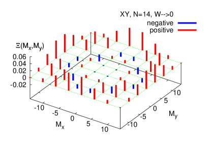
Figure 1: (Color online) $\Xi(M_{x},M_{y})$ with $W\to 0$ for the exact ground state of the XY model on a two-dimensional square lattice with $N=14$. $c\delta(0)$ [$c\in\mathbb{R}$] is represented by a vertical line with height $c$. Positive values are represented by red vertical lines, whereas negative values are represented by blue vertical lines.

Figure 2: The integral $I_{\hat{M_{x}},\hat{M}_{y}}$ of negative values of $\Xi(M_{x},M_{y})$ versus $W$ for the exact ground state of the XY model on a two-dimensional square lattice with $N=14$.

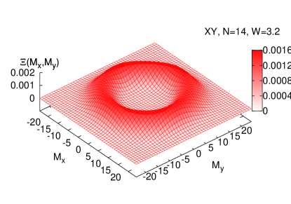
Figure 3: (Color online) $\Xi(M_{x},M_{y})$ with $W=3.2$ for the exact ground state of the XY model on a two-dimensional square lattice with $N=14$.

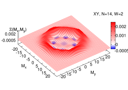
Figure 4: (Color online) $\Xi(M_{x},M_{y})$ with $W=2$ for the exact ground state of the XY model on a two-dimensional square lattice with $N=14$. Positive-valued regions are colored red, whereas negative-valued regions are colored blue.

IV.2 Heisenberg antiferromagnet

Second, we visualize the exact ground state of the Heisenberg antiferromagnet on a two-dimensional square lattice of $N$ sites. The Hamiltonian is

$$\hat{H}=\sum_{<l,l^{\prime}>}\left[\hat{\sigma}_{x}(l)\hat{\sigma}_{x}(l^{\prime})+\hat{\sigma}_{y}(l)\hat{\sigma}_{y}(l^{\prime})+\hat{\sigma}_{z}(l)\hat{\sigma}_{z}(l^{\prime})\right].$$ (22)

The ‘ground states’ obtained by the mean-field approximation are degenerate, symmetry-breaking, and separable. On the other hand, the exact ground state is unique, symmetric, and has $p=2$ if $N$ is finite Koma ; Morimae ; Horsch ; Marshall ; Miyashita . We visualize the exact ground state.

By numerical calculations, we find that $e_{1}=e_{2}=e_{3}=\mathcal{O}(N)$, $e_{i}=o(N)$ $(i\geq 4)$, $\hat{A}_{1}=\sum_{l=1}^{N}(-1)^{l}\hat{\sigma}_{x}(l)\equiv\hat{M}_{x}^{st}$, $\hat{A}_{2}=\sum_{l=1}^{N}(-1)^{l}\hat{\sigma}_{y}(l)\equiv\hat{M}_{y}^{st}$, and $\hat{A}_{3}=\sum_{l=1}^{N}(-1)^{l}\hat{\sigma}_{z}(l)\equiv\hat{M}_{z}^{st}$. Hence

$${\mathcal{S}}=\{\hat{M}_{x}^{st},\hat{M}_{y}^{st},\hat{M}_{z}^{st}\}.$$ (23)

Because $\Xi(M_{x}^{st},M_{y}^{st},M_{z}^{st})$ is hard to plot, we plot $\Xi(M_{x}^{st},M_{y}^{st})$. Because of the rotational symmetry of the model, $\Xi(M_{x}^{st},M_{y}^{st})=\Xi(M_{y}^{st},M_{z}^{st})=\Xi(M_{z}^{st},M_{x}^{st})$.

In Fig. 5, we plot $\Xi(M_{x}^{st},M_{y}^{st})$ with $W\to 0$ for $N=14$. Because $\Xi(M_{x}^{st},M_{y}^{st})$ is non-negative, it is a JPD for $\hat{M}_{x}^{st}$ and $\hat{M}_{y}^{st}$. It is also seen that many macroscopically distinct states are superposed in the ground state.

By increasing $W$, we obtain more understandable pictures. For example, in Fig. 6, we plot $\Xi(M_{x}^{st},M_{y}^{st})$ with $W=2$. It is seen that many macroscopically distinct states are so superposed that the ground state is symmetric, like the ground state of the XY model.

Figure 5: (Color online) $\Xi(M_{x}^{st},M_{y}^{st})$ with $W\to 0$ for the exact ground state of the Heisenberg antiferromagnet on a two-dimensional square lattice with $N=14$. $c\delta(0)$ [$c\in\mathbb{R}$] is represented by a vertical line with height $c$.

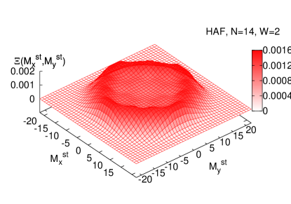
Figure 6: (Color online) $\Xi(M_{x}^{st},M_{y}^{st})$ with $W=2$ for the exact ground state of the Heisenberg antiferromagnet on a two-dimensional square lattice with $N=14$.

IV.3 Shor’s factoring algorithm

Third, we visualize a state in Shor’s factoring algorithm Shor ; Ekert . Let $I$ be an integer to be factored. We use two quantum registers, the first and the second registers, which are composed of $N_{1}$ $(2\log_{2}I\leq N_{1}<2\log_{2}I+1)$ and $N_{2}$ ($\log_{2}I\leq N_{2}<\log_{2}I+1$) qubits, respectively. We denote the total number of qubits by $N=N_{1}+N_{2}$. If the order $r$ is 6, for example, the state

$$\frac{1}{\sqrt{2^{N_{1}}}}\sum_{a=0}^{2^{N_{1}}-1}|{\sf x}^{a}~{}{\rm mod}~{}I\rangle_{2}|a\rangle_{1},$$ (24)

which appears just after the modular exponentiation, has $p=2$ Ukena ; Ukena2 . Here, $|\cdots\rangle_{1}$ and $|\cdots\rangle_{2}$ represent the first and the second registers, respectively, and ${\sf x}\ ({\sf x}<I)$ is a randomly taken integer coprime to $I$.

For the states of $r=6$, we numerically find that $e_{1}=e_{2}=\mathcal{O}(N)$, $e_{i}=o(N)$ $(i\geq 3)$, $\hat{A}_{1}=\sqrt{\frac{3}{2}}\sum_{l=2}^{N_{1}}\hat{\sigma}_{x}(l)\equiv\hat{M}_{x}^{(1)}$, and $\hat{A}_{2}=\sqrt{\frac{3}{2}}\sum_{l=2}^{N_{1}}(-1)^{l}\hat{\sigma}_{y}(l)\equiv\hat{M}_{y}^{st(1)}$ (see Appendix B). Here, the qubit states are $|0\rangle$ and $|1\rangle$ ($\hat{\sigma}_{z}|0\rangle=-|0\rangle$, $\hat{\sigma}_{z}|1\rangle=|1\rangle$). Hence

$$\mathcal{S}=\{\hat{M}_{x}^{(1)},\hat{M}^{st(1)}_{y}\}.$$ (25)

Because $\hat{M}_{x}^{(1)}$ and $\hat{M}_{y}^{st(1)}$ fluctuate macroscopically, $\hat{M}_{x}$ and $\hat{M}_{y}^{st}$ also fluctuate macroscopically Ukena2 . We here use $\hat{M}_{x}$ and $\hat{M}_{y}^{st}$ instead of $\hat{M}_{x}^{(1)}$ and $\hat{M}_{y}^{st(1)}$.

In Fig. 7, we plot $\Xi(M_{x},M_{y}^{st})$ with $W\to 0$ for $(I,{\sf x})=(21,5)$. Because $\Xi(M_{x},M_{y}^{st})$ takes negative values at some points, it is not a JPD. To see the behavior of negative values, we plot in Fig. 8 the integral $I_{\hat{M}_{x},\hat{M}_{y}^{st}}$ versus $W$. We see again that $I_{\hat{M}_{x},\hat{M}_{y}^{st}}$ approaches 0 as $W$ is increased. $\Xi(M_{x},M_{y}^{st})$ therefore becomes a cgJPD if $W$ is sufficiently large.

In Fig. 9, we plot $\Xi(M_{x},M_{y}^{st})$ with $W=1.4$. Because $\Xi(M_{x},M_{y}^{st})$ is non-negative, it is a cgJPD for $\hat{M}_{x}$ and $\hat{M}_{y}^{st}$. There are four peaks, which represent a superposition of approximately four macroscopically distinct states.

In Fig. 10, we plot $\Xi(M_{x},M_{y}^{st})$ with smaller $W$, $W=1$. In this case, there is a negative-valued region. However, because $|I_{\hat{M}_{x},\hat{M}_{y}^{st}}|$ is small, $\Xi(M_{x},M_{y}^{st})$ is interpreted as a cgQJPD. $\Xi(M_{x},M_{y}^{st})$ again represents four peaks. We have also observed such a four-peak structure for some other values of $(I,{\sf x})$’s.

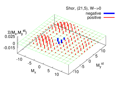
Figure 7: (Color online) $\Xi(M_{x},M_{y}^{st})$ with $W\to 0$ for the state just after the modular exponentiation with $(I,{\sf x})=(21,5)$. $c\delta(0)$ [$c\in\mathbb{R}$, $c>0$] is represented by a vertical line with height $c$. $c\delta(0)$ [$c\in\mathbb{R}$, $c<0$] is represented by a vertical line with height $10c$, in order to make negative values more visible. Positive values are represented by red vertical lines, whereas negative values are represented by blue vertical lines.

Figure 8: The integral $I_{\hat{M}_{x},\hat{M}_{y}^{st}}$ of negative values of $\Xi(M_{x},M_{y}^{st})$ versus $W$ for the state just after the modular exponentiation with $(I,{\sf x})=(21,5)$.

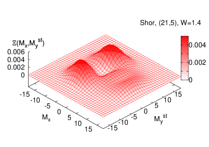
Figure 9: (Color online) $\Xi(M_{x},M_{y}^{st})$ with $W=1.4$ for the state just after the modular exponentiation with $(I,{\sf x})=(21,5)$.

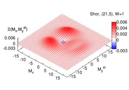
Figure 10: (Color online) $\Xi(M_{x},M_{y}^{st})$ with $W=1$ for the state just after the modular exponentiation with $(I,{\sf x})=(21,5)$. Positive-valued regions are colored red, whereas negative-valued regions are colored blue. In order to make negative regions more visible, negative values are multiplied by 10.

IV.4 Grover’s quantum search algorithm

Finally, we visualize a state in Grover’s quantum search algorithm Grover ; Nielsen . Let us consider the problem of finding a solution to the equation $f(x)=1$ among $2^{N}$ possibilities, where $f(x)$ is a function, $f:\{0,1,\cdots,2^{N}-1\}\to\{0,1\}$. These $2^{N}$ possibilities are indexed by $2^{N}$ computational basis states, which are tensor products of $|0\rangle$ or $|1\rangle$ of $N$ qubits. Here, $\hat{\sigma}_{z}|0\rangle=-|0\rangle$ and $\hat{\sigma}_{z}|1\rangle=|1\rangle$. Let $|G_{k}\rangle$ be the state which appears after $k$ Grover iterations. It was shown that if the number of the solutions is $\mathcal{O}(N^{0})$, $|G_{k}\rangle$’s whose $k$ satisfies

$$\delta\leq\frac{4k+2}{\sqrt{2^{N}}}\leq\pi-\delta$$ (26)

have $p=2$, irrespective of which numbers are the solutions Ukena2 . Here, $\delta$ is an arbitrary small positive constant being independent of $N$.

To be definite, we assume that the state $|1^{\otimes N}\rangle$ indexes the solution. Then $|G_{k}\rangle$ is written as

$$|G_{k}\rangle = \cos\left(\frac{2k+1}{2}\theta\right)\frac{1}{\sqrt{2^{N}-1}}\left[|0^{\otimes N}\rangle+\cdots\right]$$ (27)

$$~{}+\sin\left(\frac{2k+1}{2}\theta\right)|1^{\otimes N}\rangle,$$

where $\cos\frac{\theta}{2}=\sqrt{(2^{N}-1)/2^{N}}$, and $\left[|0^{\otimes N}\rangle+\cdots\right]$ is the equal-weight superposition of all computational basis states except for $|1^{\otimes N}\rangle$. Among many $k$’s which satisfy Eq. (26), we use $k=R/2$ for even $R$, and $k=R/2+0.5$ for odd $R$, where $R\equiv{\rm CI}\left(\theta^{-1}\arccos\sqrt{2^{-N}}\right)$ is the number of total Grover iterations. Here, ${\rm CI}(x)$ denotes the integer closest to the real number $x$.

We numerically find that $e_{1}=\mathcal{O}(N)$, $e_{i}=o(N)$ $(i\geq 2)$, and $\hat{A}_{1}=\sum_{l=1}^{N}\left[\frac{-1}{\sqrt{2}}\hat{\sigma}_{x}(l)+\frac{1}{\sqrt{2}}\hat{\sigma}_{z}(l)\right]\equiv\hat{M}_{x\mathchar 45\relax z}$ (see Appendix B). Hence

$${\mathcal{S}}=\{\hat{M}_{x\mathchar 45\relax z}\}.$$ (28)

Because $\mathcal{S}$ has only one element, the macroscopic superposition can be visualized by plotting the probability density $\langle G_{k}|{\mathcal{P}}_{\hat{M}_{x\mathchar 45\relax z}}(M_{x\mathchar 45\relax z})|G_{k}\rangle$. However, because it is more interesting to plot $\Xi(M_{x\mathchar 45\relax z},A)$, where $\hat{A}$ is a hermitian additive operator, we plot $\Xi(M_{x\mathchar 45\relax z},M_{y})$ in this paper. The shape of $\langle G_{k}|{\mathcal{P}}_{\hat{M}_{x\mathchar 45\relax z}}(M_{x\mathchar 45\relax z})|G_{k}\rangle$ can be deduced from that of $\Xi(M_{x\mathchar 45\relax z},M_{y})$.

In Fig. 11, we plot $\Xi(M_{x\mathchar 45\relax z},M_{y})$ with $W\to 0$ for $N=12$. Because $\Xi$ takes negative values at some points, it is not a JPD. To see the behavior of the negative values, we plot in Fig. 12 the integral $I_{\hat{M}_{x\mathchar 45\relax z},\hat{M}_{y}}$ versus $W$. $I_{\hat{M}_{x\mathchar 45\relax z},\hat{M}_{y}}$ approaches 0 as $W$ is increased. $\Xi(M_{x\mathchar 45\relax z},M_{y})$ therefore becomes a cgJPD for $\hat{M}_{x\mathchar 45\relax z}$ and $\hat{M}_{y}$ if $W$ is sufficiently large.

In Fig. 13, we plot $\Xi(M_{x\mathchar 45\relax z},M_{y})$ with $W=2$. Because there are small negative-valued regions, it is a cgQJPD. It is seen that the state is approximately a cat state, i.e., an equal-weight superposition of two macroscopically distinct states. Although this information can also be obtained by plotting $\langle G_{k}|\mathcal{P}_{\hat{M}_{x\mathchar 45\relax z}}(M_{x\mathchar 45\relax z})|G_{k}\rangle$, we can see interesting structures of $|G_{k}\rangle$, including negative-valued regions, by plotting $\Xi(M_{x\mathchar 45\relax z},M_{y})$.

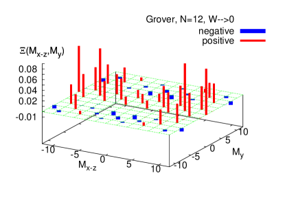
Figure 11: (Color online) $\Xi(M_{x\mathchar 45\relax z},M_{y})$ with $W\to 0$ for a state in Grover’s quantum search algorithm with $N=12$. $c\delta(0)$ [$c\in\mathbb{R}$] is represented by a vertical line with height $c$. Positive values are represented by red vertical lines, whereas negative values are represented by blue vertical lines.

Figure 12: The integral $I_{\hat{M}_{x\mathchar 45\relax z},\hat{M}_{y}}$ of negative values of $\Xi(M_{x\mathchar 45\relax z},M_{y})$ versus $W$ for a state in Grover’s quantum search algorithm with $N=12$.

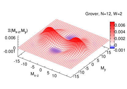
Figure 13: (Color online) $\Xi(M_{x\mathchar 45\relax z},M_{y})$ with $W=2$ for a state in Grover’s quantum search algorithm with $N=12$. Positive-valued regions are colored red, whereas negative-valued regions are colored blue.

V discussion

V.1 Non-negativity of $\Xi$

In the previous section, we have observed that an appropriate value of $W$ which makes $\Xi$ non-negative largely depends on the quantum state to be visualized. For example, $\Xi(M_{x},M_{y})$ for the ground state of the XY model becomes non-negative with $W=3.2$, whereas $\Xi(M_{x},M_{y}^{st})$ for the state in Shor’s factoring algorithm becomes non-negative with smaller $W$, $W=1.4$, for the same value of $N$. Furthermore, $\Xi(M_{x}^{st},M_{y}^{st})$ for the ground state of the Heisenberg antiferromagnet is non-negative with any $W$. Therefore, in general, one must find an appropriate value of $W$ a posteriori.

However, it is worth mentioning that a sufficient magnitude of $W$ which makes $\Xi$ non-negative seems to be $\mathcal{O}(N)$. To see this, consider the following three examples.

Example 1: In Figs. 14 and 15, we plot $I_{\hat{M}_{x\mathchar 45\relax z},\hat{M}_{y}}$ versus $N$ for $|G_{k}\rangle$ of Eq. (27) with $W=\mathcal{O}(N)$ and $W=\mathcal{O}(\sqrt{N})$, respectively. Here, $k=R/2$ for even $R$, and $k=R/2+0.5$ for odd $R$. It is seen that $I_{\hat{M}_{x\mathchar 45\relax z},\hat{M}_{y}}$ approaches 0 as $N$ is increased if $W=\mathcal{O}(N)$, whereas it does not approach 0 if $W=\mathcal{O}(\sqrt{N})$.

Example 2: In Fig. 16, we plot $\Xi(M_{x},M_{y})$ for the separable state $|0^{\otimes N}\rangle$ with $W=1.5$ and $N=14$. Here, $\hat{\sigma}_{z}|0\rangle=-|0\rangle$. There are negative-valued regions. In Figs. 17 and 18, we plot $I_{\hat{M}_{x},\hat{M}_{y}}$ versus $N$ with $W=\mathcal{O}(N)$ and $W=\mathcal{O}(\sqrt{N})$, respectively. We can see again that $I_{\hat{M}_{x},\hat{M}_{y}}$ approaches 0 as $N$ is increased if $W=\mathcal{O}(N)$, whereas it does not approach 0 if $W=\mathcal{O}(\sqrt{N})$.

Example 3: For the cat state $\frac{1}{\sqrt{2}}|0^{\otimes N}\rangle+\frac{1}{\sqrt{2}}|1^{\otimes N}\rangle$, in which $\hat{M}_{z}$ fluctuates macroscopically, $\Xi(M_{z},M_{x})$ and $\Xi(M_{z},M_{y})$ are non-negative. On the other hand, $\Xi(M_{x},M_{y})$ can take negative values. In Fig. 19, we plot $\Xi(M_{x},M_{y})$ with $W=1.5$ and $N=14$. It is seen that there are negative-valued regions. In Figs. 20 and 21, we plot $I_{\hat{M}_{x},\hat{M}_{y}}$ with $W=\mathcal{O}(N)$ and $W=\mathcal{O}(\sqrt{N})$, respectively. $I_{\hat{M}_{x},\hat{M}_{y}}$ again approaches 0 as $N$ is increased if $W=\mathcal{O}(N)$, whereas it does not approach 0 if $W=\mathcal{O}(\sqrt{N})$.

From these (and some other) examples, it is expected that $\mathcal{O}(N)$ is a sufficient magnitude of $W$ which makes $\Xi$ non-negative for sufficiently large $N$. This expectation is reasonable, because $W=\mathcal{O}(N)$ means that the relative error of a measurement is independent of the system size $N$, which is a usual situation for macroscopic systems.

Whether $\Xi(A_{1},\cdots,A_{m})$ is non-negative or not depends also on which additive operators $\hat{A}_{1},\cdots,\hat{A}_{m}$ are used. For the ground state of the XY model, for example, if we use $\hat{M}_{x}$ and $\hat{M}_{z}$ instead of $\hat{M}_{x}$ and $\hat{M}_{y}$, $\Xi(M_{x},M_{z})$ is non-negative with any $W$, because the ground state is an eigenstate of $\hat{M}_{z}$ corresponding to the eigenvalue $M_{z}=0$, hence $\Xi(M_{x},M_{z})=\Xi_{\hat{M}_{x}}(M_{x})w(M_{z})\geq 0$.

At the time of writing, however, we do not know a method of finding hermitian additive operators and $W$ which make $\Xi$ non-negative for a given state. To find such a method will be a subject of future studies.

V.2 Negative-valued regions of $\Xi$

If $[\hat{A},\hat{B}]=0$, $\Xi(A,B)$ is non-negative. It is therefore expected that negative-valued regions of $\Xi$ represent some quantum natures, like those of the Wigner distribution function.

It seems that superposition of macroscopically distinct states studied in this paper is not directly related to negative-valued regions. For example, $\Xi(M_{x}^{st},M_{y}^{st})$ is non-negative with any $W$ for the ground state of the Heisenberg antiferromagnet, which has $p=2$.

In the previous subsection, on the other hand, we have seen that $\Xi(M_{x},M_{y})$ has negative-valued regions for the separable state $|0^{\otimes N}\rangle$. Because the separable state has no quantum nature other than the quantum coherence within each site, the negative-valued regions should represent this quantum coherence. This expectation is reasonable, because $\Xi(M_{x},M_{y})$ is non-negative with any $W$ for the random state $\hat{\rho}_{r}\equiv\frac{1}{2^{N}}\hat{1}$, which has neither entanglement nor quantum coherence. Here, we provisionally define $\Xi$ for a mixed state $\hat{\rho}$ by $\Xi(A,B)\equiv\frac{1}{2}{\rm Tr}\hat{\rho}[\overline{\mathcal{P}}_{\hat{A}}(A)\overline{\mathcal{P}}_{\hat{B}}(B)+\overline{\mathcal{P}}_{\hat{B}}(B)\overline{\mathcal{P}}_{\hat{A}}(A)]$.

Detailed analysis of negative-valued regions is, however, beyond the scope of the present paper. It will also be a subject of future studies.

Figure 14: The integral $I_{\hat{M}_{x\mathchar 45\relax z},\hat{M}_{y}}$ of negative values of $\Xi(M_{x\mathchar 45\relax z},M_{y})$ versus $N$ with $W=N/6$ and $W=N/8$ for states in Grover’s quantum search algorithm. Lines are guides to the eye.

Figure 15: The integral $I_{\hat{M}_{x\mathchar 45\relax z},\hat{M}_{y}}$ of negative values of $\Xi(M_{x\mathchar 45\relax z},M_{y})$ versus $N$ with $W=\sqrt{N}$ and $W=\sqrt{0.5N}$ for states in Grover’s quantum search algorithm.

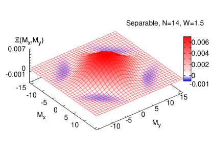
Figure 16: (Color online) $\Xi(M_{x},M_{y})$ with $W=1.5$ for the separable state $|0^{\otimes N}\rangle$ with $N=14$. Positive-valued regions are colored red, whereas negative-valued regions are colored blue.

Figure 17: The integral $I_{\hat{M}_{x},\hat{M}_{y}}$ of negative values of $\Xi(M_{x},M_{y})$ versus $N$ with $W=N/6$, $W=N/8$, and $W=N/10$ for separable states $|0^{\otimes N}\rangle$. Lines are guides to the eye.

Figure 18: The integral $I_{\hat{M}_{x},\hat{M}_{y}}$ of negative values of $\Xi(M_{x},M_{y})$ versus $N$ with $W=\sqrt{N}$ and $W=\sqrt{0.5N}$ for separable states $|0^{\otimes N}\rangle$.

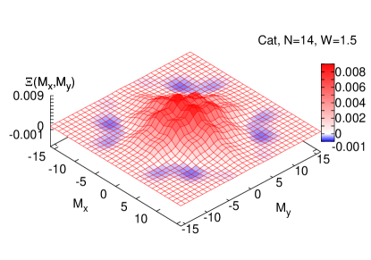
Figure 19: (Color online) $\Xi(M_{x},M_{y})$ with $W=1.5$ for the cat state $\frac{1}{\sqrt{2}}|0^{\otimes N}\rangle+\frac{1}{\sqrt{2}}|1^{\otimes N}\rangle$ with $N=14$. Positive-valued regions are colored red, whereas negative-valued regions are colored blue.

Figure 20: The integral $I_{\hat{M}_{x},\hat{M}_{y}}$ of negative values of $\Xi(M_{x},M_{y})$ versus $N$ with $W=N/6$, $W=N/8$, and $W=N/10$ for cat states $\frac{1}{\sqrt{2}}|0^{\otimes N}\rangle+\frac{1}{\sqrt{2}}|1^{\otimes N}\rangle$. Lines are guides to the eye.

Figure 21: The integral $I_{\hat{M}_{x},\hat{M}_{y}}$ of negative values of $\Xi(M_{x},M_{y})$ versus $N$ with $W=\sqrt{N}$ and $W=\sqrt{0.5N}$ for cat states $\frac{1}{\sqrt{2}}|0^{\otimes N}\rangle+\frac{1}{\sqrt{2}}|1^{\otimes N}\rangle$.

Appendix A $e_{1}=\mathcal{O}(N^{p-1})$

In this appendix, we show that $e_{1}=\mathcal{O}(N^{p-1})$. For a given pure state $|\psi\rangle$, let $\{\tilde{c}_{\alpha l}^{~{}1}\}\in\mathbb{C}^{3N}$ be an eigenvector of the VCM corresponding to the maximum eigenvalue $e_{1}$. We normalize it as $\sum_{\alpha l}|\tilde{c}_{\alpha l}^{~{}1}|^{2}=N$. From the eigenvector, we construct the operator:

$$\hat{\sf A}_{1}\equiv\sum_{\alpha l}\tilde{c}_{\alpha l}^{~{}1}\hat{\sigma}_{\alpha}(l).$$ (29)

If it is hermitian and all $\tilde{c}_{\alpha l}^{~{}1}$’s are independent of $N$, it gives the maximum of Eq. (1). Therefore, $\max_{\hat{A}}\langle\psi|(\Delta\hat{A})^{2}|\psi\rangle=e_{1}N$ in Eq. (1). Hence $e_{1}=\mathcal{O}(N^{p-1})$.

If $\hat{\sf A}_{1}$ is non-hermitian and all $\tilde{c}_{\alpha l}^{~{}1}$’s are independent of $N$, we decompose it as: $\hat{\sf A}_{1}=\hat{A}_{1}^{\rm re}+i\hat{A}_{1}^{\rm im}$, where $\hat{A}_{1}^{\rm re}\equiv(\hat{\sf A}_{1}+\hat{\sf A}_{1}^{\dagger})/2$ and $\hat{A}_{1}^{\rm im}\equiv(\hat{\sf A}_{1}-\hat{\sf A}_{1}^{\dagger})/2i$. Then $\langle\psi|(\Delta\hat{A}_{1}^{\rm re})^{2}|\psi\rangle=\mathcal{O}(e_{1}N)$ or $\langle\psi|(\Delta\hat{A}_{1}^{\rm im})^{2}|\psi\rangle=\mathcal{O}(e_{1}N)$, because

$$\|\Delta\hat{\sf A}_{1}|\psi\rangle\| = \|\Delta\hat{A}_{1}^{\rm re}|\psi\rangle+i\Delta\hat{A}_{1}^{\rm im}|\psi\rangle\|$$ (30)

$$\leq \|\Delta\hat{A}_{1}^{\rm re}|\psi\rangle\|+\|\Delta\hat{A}_{1}^{\rm im}|\psi\rangle\|.$$

Assume that $\langle\psi|(\Delta\hat{A}_{1}^{\rm re})^{2}|\psi\rangle=\mathcal{O}(e_{1}N)$. Because $\hat{\sf A}_{1}$ is additive, $\hat{A}_{1}^{\rm re}$ is also additive. Then $\max_{\hat{A}}\langle\psi|(\Delta\hat{A})^{2}|\psi\rangle=\mathcal{O}(e_{1}N)$ in Eq. (1). Hence $e_{1}=\mathcal{O}(N^{p-1})$.

If some $\tilde{c}_{\alpha l}^{~{}1}$’s depend on $N$, we compose the additive operator

$$\hat{A}_{1}\equiv\sum_{\alpha l}c_{\alpha l}^{1}\hat{\sigma}_{\alpha}(l),$$ (31)

where $\{c_{\alpha l}^{1}\}$ is obtained by taking an appropriate limit of $\{\tilde{c}_{\alpha l}^{~{}1}\}$ as described in Appendix B. It can be shown that $\langle\psi|\Delta\hat{A}_{1}^{\dagger}\Delta\hat{A}_{1}|\psi\rangle=\mathcal{O}(e_{1}N)$. In fact, by defining $\tilde{d}_{\alpha l}^{~{}1}\equiv\tilde{c}_{\alpha l}^{~{}1}-c_{\alpha l}^{1}$,

$$\langle\psi|\Delta\hat{A}_{1}^{\dagger}\Delta\hat{A}_{1}|\psi\rangle = \sum_{\alpha l\beta l^{\prime}}c_{\alpha l}^{1*}c_{\beta l^{\prime}}^{1}V_{\alpha l,\beta l^{\prime}}$$ (32)

$$= \sum_{\alpha l\beta l^{\prime}}(\tilde{c}_{\alpha l}^{~{}1*}-\tilde{d}_{\alpha l}^{~{}1*})(\tilde{c}_{\beta l^{\prime}}^{~{}1}-\tilde{d}_{\beta l^{\prime}}^{~{}1})V_{\alpha l,\beta l^{\prime}}$$

$$= e_{1}N+e_{1}o(N)+\sum_{\alpha l\beta l^{\prime}}\tilde{d}_{\alpha l}^{~{}1*}\tilde{d}_{\beta l^{\prime}}^{~{}1}V_{\alpha l,\beta l^{\prime}}$$

$$= \mathcal{O}(e_{1}N),$$

where we have used the facts that $\{\tilde{c}_{\alpha l}^{~{}1}\}$ is an eigenvector of the VCM corresponding to $e_{1}$, that $\sum_{\alpha l}|\tilde{c}_{\alpha l}^{~{}1}|^{2}=N$, that $\tilde{d}_{\alpha l}^{~{}1}=o(N^{0})$, and that $0\leq\sum_{\alpha l\beta l^{\prime}}\tilde{d}_{\alpha l}^{~{}1*}\tilde{d}_{\beta l^{\prime}}^{~{}1}V_{\alpha l,\beta l^{\prime}}\leq e_{1}N$. If $\hat{A}_{1}$ is hermitian, $\max_{\hat{A}}\langle\psi|(\Delta\hat{A})^{2}|\psi\rangle=\mathcal{O}(e_{1}N)$ in Eq. (1). Hence $e_{1}=\mathcal{O}(N^{p-1})$. If $\hat{A}_{1}$ is not hermitian, its real or imaginary part gives $\mathcal{O}(e_{1}N)$ fluctuation. Therefore, $\max_{\hat{A}}\langle\psi|(\Delta\hat{A})^{2}|\psi\rangle=\mathcal{O}(e_{1}N)$ in Eq. (1). Hence $e_{1}=\mathcal{O}(N^{p-1})$.

In conclusion, we have shown that $e_{1}=\mathcal{O}(N^{p-1})$.

Appendix B Composition of $\{c_{\alpha l}^{i}\}$ from $\{\tilde{c}_{\alpha l}^{~{}i}\}$

By diagonalizing the VCM, one obtains $\{\tilde{c}_{\alpha l}^{~{}i}\}\in\mathbb{C}^{3N}$ corresponding to $e_{i}$. Each element $\tilde{c}_{\alpha l}^{~{}i}$ generally depends on $N$, whereas $c_{\alpha l}^{i}$’s composing the additive operator $\hat{A}_{i}$ through Eq. (18) should be independent of $N$. We can deduce $c_{\alpha l}^{i}$ from $\tilde{c}_{\alpha l}^{~{}i}$ simply as follows.

Let us define a parameter $\nu\equiv l/N$, and denote $\tilde{c}_{\alpha l}^{~{}i}$ by $\tilde{c}_{\alpha\nu}^{~{}i}(N)$. We take the following limit:

$$\lim_{N^{\prime}\to\infty}\tilde{c}_{\alpha\nu}^{~{}i}(N^{\prime})\equiv c_{\alpha}^{i}(\nu),$$ (33)

where $\nu$ is kept constant in this limit. Then, $c_{\alpha l}^{i}$ is given by $c_{\alpha l}^{i}=c_{\alpha}^{i}(l/N)$. Note that a small number [$=O(N^{0})$] of elements among $3N$ elements of $\{c_{\alpha l}^{i}\}$ can be modified, because it does not alter the leading term (with respect to $N$) of $\langle\psi|\Delta\hat{A}_{i}^{\dagger}\Delta\hat{A}_{i}|\psi\rangle$. Using this property, we can adjust $\hat{A}_{i}$ for our convenience.

For the state of Eq. (24) with $r=6$, for example,

$$\tilde{c}^{~{}1}_{\alpha l}=\left\{\begin{array}[]{cc}\sqrt{N/(N_{1}-1)}&(\alpha=x;\ 2\leq l\leq N_{1}),\\ 0&({\rm others}),\end{array}\right.$$ (36)

$$\tilde{c}^{~{}2}_{\alpha l}=\left\{\begin{array}[]{cc}(-1)^{l}\sqrt{N/(N_{1}-1)}&(\alpha=y;\ 2\leq l\leq N_{1}),\\ 0&({\rm others}).\end{array}\right.$$ (39)

We therefore obtain

$$c^{1}_{\alpha l}=\left\{\begin{array}[]{cc}\sqrt{3/2}&(\alpha=x;\ 1\leq l\leq N_{1}),\\ 0&({\rm others}),\end{array}\right.$$ (42)

$$c^{2}_{\alpha l}=\left\{\begin{array}[]{cc}(-1)^{l}\sqrt{3/2}&(\alpha=y;\ 1\leq l\leq N_{1}),\\ 0&({\rm others}).\end{array}\right.$$ (45)

Or, we can modify the $l=1$ terms of these results as $c^{1}_{\alpha 1}=\ c^{2}_{\alpha 1}=0$ in accordance with the $l=1$ terms of Eqs. (36) and (39). We have employed the latter forms in Sec. IV.3.

Moreover, for $|G_{k}\rangle$ with $k=R/2$ (even $R$) or $k=R/2+0.5$ (odd $R$),

$$\tilde{c}^{~{}1}_{\alpha l}=\left\{\begin{array}[]{cc}-a/\sqrt{a^{2}+b^{2}+c^{2}}&(\alpha=x;~{}1\leq l\leq N),\\ ib/\sqrt{a^{2}+b^{2}+c^{2}}&(\alpha=y;~{}1\leq l\leq N),\\ c/\sqrt{a^{2}+b^{2}+c^{2}}&(\alpha=z;~{}1\leq l\leq N).\end{array}\right.$$ (49)

Here, $a$, $b$ and $c$ are real numbers which depend on $N$. It is numerically shown that $\lim_{N\to\infty}(a-c)=0$ and $\lim_{N\to\infty}b/\sqrt{a^{2}+b^{2}+c^{2}}=0$. We therefore obtain

$$c^{1}_{\alpha l}=\left\{\begin{array}[]{cc}-1/\sqrt{2}&(\alpha=x;~{}1\leq l\leq N),\\ 0&(\alpha=y;~{}1\leq l\leq N),\\ 1/\sqrt{2}&(\alpha=z;~{}1\leq l\leq N),\end{array}\right.$$ (53)

which has been used in Sec. IV.4.

Appendix C $\hat{A}_{i}$ fluctuates macroscopically if and only if $e_{i}=\mathcal{O}(N)$

In this appendix, we show that $\hat{A}_{i}$ of Eq. (18) fluctuates macroscopically if and only if $e_{i}=\mathcal{O}(N)$. Using $c_{\alpha l}^{i}$ of Appendix B, we define $\tilde{d}_{\alpha l}^{~{}i}\equiv\tilde{c}_{\alpha l}^{~{}i}-c_{\alpha l}^{i}$. Then

$$\langle\psi|\Delta\hat{A}_{i}^{\dagger}\Delta\hat{A}_{i}|\psi\rangle = \sum_{\alpha l\beta l^{\prime}}c_{\alpha l}^{i*}c_{\beta l^{\prime}}^{i}V_{\alpha l,\beta l^{\prime}}$$ (54)

$$= \sum_{\alpha l\beta l^{\prime}}(\tilde{c}_{\alpha l}^{~{}i*}-\tilde{d}_{\alpha l}^{~{}i*})(\tilde{c}_{\beta l^{\prime}}^{~{}i}-\tilde{d}_{\beta l^{\prime}}^{~{}i})V_{\alpha l,\beta l^{\prime}}$$

$$= e_{i}N+e_{i}o(N)+o(N^{2}),$$

where we have used the facts that $\{\tilde{c}_{\alpha l}^{~{}i}\}$ is an eigenvector of the VCM corresponding to $e_{i}$, that $\sum_{\alpha l}|\tilde{c}_{\alpha l}^{~{}i}|^{2}=N$, and that $\tilde{d}_{\alpha l}^{~{}i}=o(N^{0})$. Therefore, if $e_{i}=\mathcal{O}(N)$ then $\langle\psi|\Delta\hat{A}_{i}^{\dagger}\Delta\hat{A}_{i}|\psi\rangle=\mathcal{O}(N^{2})$. On the other hand, if $e_{i}=o(N)$ then $\langle\psi|\Delta\hat{A}_{i}^{\dagger}\Delta\hat{A}_{i}|\psi\rangle=o(N^{2})$.

Appendix D any macroscopically fluctuating additive operator includes an element of $\mathcal{S}$

For an additive operator $\hat{A}=\sum_{\alpha l}c_{\alpha l}\hat{\sigma}_{\alpha}(l)$, the coefficient vector $\{c_{\alpha l}\}\in\mathbb{C}^{3N}$ can be expressed as a linear combination of $\{\tilde{c}_{\alpha l}^{~{}i}\}$’s: $c_{\alpha l}=\sum_{i=1}^{3N}\xi_{i}\tilde{c}_{\alpha l}^{~{}i}$, where $\xi_{i}$’s are coefficients satisfying $\sum_{i}|\xi_{i}|^{2}=\mathcal{O}(N^{0})$. Assume that $\xi_{i}=o(N^{0})$ if $e_{i}=\mathcal{O}(N)$ ($i=1,\cdots,3N$). Then

$$\langle\psi|\Delta\hat{A}^{\dagger}\Delta\hat{A}|\psi\rangle=N\sum_{i}|\xi_{i}|^{2}e_{i}=o(N^{2}),$$ (55)

where we have used the facts that $\{\tilde{c}_{\alpha l}^{~{}i}\}$’s are orthogonal eigenvectors of the VCM, and that $\sum_{\alpha l}|\tilde{c}_{\alpha l}^{~{}i}|^{2}=N$. Equation (55) shows that $\hat{A}$ does not fluctuate macroscopically.

In other words, if $\hat{A}$ fluctuates macroscopically, its coefficient vector $\{c_{\alpha l}\}$ includes at least one $\{\tilde{c}_{\alpha l}^{~{}i}\}$ whose $e_{i}=\mathcal{O}(N)$ as a component of the linear combination with the weight $\xi_{i}=\mathcal{O}(N^{0})$. Therefore,

$$\hat{A} = \sum_{\alpha l}[\cdots+\xi_{i}\tilde{c}^{~{}i}_{\alpha l}\hat{\sigma}_{\alpha}(l)+\cdots]$$ (56)

$$= \sum_{\alpha l}[\cdots+\xi_{i}(c^{i}_{\alpha l}+\tilde{d}^{~{}i}_{\alpha l})\hat{\sigma}_{\alpha}(l)+\cdots]$$

$$= \cdots+\xi_{i}\hat{A}_{i}+\cdots,$$

which shows that $\hat{A}$ includes $\hat{A}_{i}$ (hence also $\hat{A}_{i}^{\rm re}$ and $\hat{A}_{i}^{\rm im}$) with the weight $\xi_{i}=\mathcal{O}(N^{0})$. In this sense, at least one element of $\mathcal{S}$ is ‘included’ in $\hat{A}$, if $\hat{A}$ fluctuates macroscopically.

References

- (1) E. Wigner, Phys. Rev. 40, 749 (1932).
- (2) K. Husimi, Proc. Phys. Math. Soc. Jpn. 22, 264 (1940).
- (3) For example, L. Mandel and E. Wolf, Optical Coherence and Quantum Optics (Cambridge University Press, Cambridge, 1995).
- (4) W. K. Wootters, Ann. Phys. 176, 1 (1987).
- (5) U. Leonhardt, Phys. Rev. A 53, 2998 (1996).
- (6) J. H. Hannay and M. V. Berry, Physica D 1, 267 (1980).
- (7) A. M. F. Rivas and A. M. Ozorio de Almeida, Ann. Phys. 276, 223 (1999).
- (8) P. W. Shor, in Proceedings of the 35th Annual Symposium on the Foundations of Computer Science, edited by S. Goldwasser (IEEE Computer Society, Los Alamitos, CA, 1994), p. 124.
- (9) L. K. Grover, Phys. Rev. Lett. 79, 325 (1997).
- (10) M. A. Nielsen and I. L. Chuang, Quantum computation and Quantum Information (Cambridge University Press, Cambridge, 2000).
- (11) A. Ekert and R. Jozsa, Rev. Mod. Phys. 68, 733 (1996).
- (12) E. Schrödinger, Naturwissenschaften. 23, 807, 823, 844 (1935).
- (13) A. J. Leggett, Prog. Theor. Phys., Suppl. 69, 80 (1980).
- (14) Y. Nakamura, Y. A. Pashkin, and J. S. Tsai, Nature 398, 786 (1999).
- (15) J. R. Friedman, V. Patel, W. Chen, S. K. Tolpygo, and J. E. Lukens, Nature 406, 43 (2000).
- (16) C. H. van der Wal, A. C. J. ter Haar, F. K. Wilhelm, R. N. Schouten, C. J. P. M. Harmans, T. P. Orlando, S. Lloyd, and J. E. Mooij, Science 290, 773 (2000).
- (17) N. D. Mermin, Phys. Rev. Lett. 65, 1838 (1990).
- (18) H. Wakita, Prog. Theor. Phys. 23, 32 (1960).
- (19) A. A. Grib, E. V. Damaskinskii, and V. M. Maksimov, Usp. Fiz. Nauk 102, 587 (1970); [Sov. Phys. Usp. 13, 798 (1971)].
- (20) W. Dür, C. Simon, and J. I. Cirac, Phys. Rev. Lett. 89, 210402 (2002).
- (21) A. Shimizu and T. Miyadera, Phys. Rev. Lett. 89, 270403 (2002).
- (22) A. Ukena and A. Shimizu, Phys. Rev. A 69, 022301 (2004).
- (23) A. Ukena and A. Shimizu, quant-ph/0505057.
- (24) T. Morimae, A. Sugita, and A. Shimizu, Phys. Rev. A 71, 032317 (2005).
- (25) A. Shimizu and T. Morimae, Phys. Rev. Lett. 95, 090401 (2005).
- (26) A. Shimizu and T. Miyadera, J. Phys. Soc. Jpn. 71, 56 (2002).
- (27) A. Sugita and A. Shimizu, J. Phys. Soc. Jpn. 74, 1883 (2005).
- (28) In this paper, we use three symbols , , and to represent asymptotic behavior of a function as : if constant , if is finite, and if .
- (29) This point can be seen by the following trivial example. Dividing by a large number yields However, the noncommutativity of and can be detected by high-resolution experiments.
- (30) A. Shimizu and T. Miyadera, Phys. Rev. E 64, 056121 (2001).
- (31) T. Koma and H. Tasaki, J. Stat. Phys. 76, 745 (1994).
- (32) J. Oitmaa and D. D. Betts, Can. J. Phys. 56, 897 (1978).
- (33) S. Miyashita, in Quantum Simulations of Condensed Matter Phenomena, edited by J. D. Doll and J. E. Gubernatis (World Scientific, Singapore, 1990).
- (34) V. I. Yukalov, Laser Phys. 16, 511 (2006).
- (35) P. Horsch and W. von der Linden, Z. Phys. B 72, 181 (1988).
- (36) W. Marshall, Proc. Roy. Soc. A 232, 48 (1955).