Exactly solvable associated Lamé potentials and supersymmetric transformations

Abstract

A systematic procedure to derive exact solutions of the associated Lamé equation for an arbitrary value of the energy is presented. Supersymmetric transformations in which the seed solutions have factorization energies inside the gaps are used to generate new exactly solvable potentials; some of them exhibit an interesting property of periodicity defects.

, Accepted in Annals of Physics

1 Introduction

The exactly solvable potentials of the one-dimensional Schrödinger equation are important due to the fact that the full physical information of the system is encoded in a small number of analytical expressions. Moreover, they can be used to test the convergence of the numerical methods as well as to be the departure point for applying the widely used perturbative techniques. By exact solvability we mean that the stationary Schrödinger equation for the involved potential (when it is periodic) admits analytic solutions for energies in the allowed bands as well as for energies in the gaps.

A remarkable fact, the existence of a class of potentials which are intermediate between the exactly solvable ones and those just solvable through numerical techniques, was realized since the date back to 80 s of past century. Nowadays they are known as quasi-exactly solvable potentials, and their characteristic property is that there exist compact analytical expressions of physical information for only a part of the system spectrum. This means that there are some missing features of these models which just can be numerically determined. A big effort has been observed for years in identifying the potentials which are quasi-exactly solvable, and gradually it started to dominate the conviction that this class includes the associated Lamé potentials [1, 2, 3, 4, 5, 6, 7, 8], among others. However, some signs have been recently noticed indicating that the associated Lamé potentials for some integer values of the parameter pair $(m,\ell)$ belong as well to the exactly solvable class. Recently, we proposed [7] an ansatz through which one can implement a fitting procedure to automatically fix the values of $m,\ \ell$, the ansatz parameters and consequently the analytic solutions of the associated Lamé equation. Unfortunately, that procedure was not completely systematic in the sense that one has to compute case by case for each pair of values of $(m,\ell)$ to find the general solution by adopting the natural modification of the ansatz.

On the other hand, it seems interesting to enlarge the exactly solvable class of potentials departing from a given initial one. Several procedures are available to do this, and the simplest one is called supersymmetric quantum mechanics (SUSY QM) [9, 10, 11, 12, 13, 14, 15, 16]. In this approach there is a differential operator of order $k$ intertwining the initial and final Hamiltonians, the main ingredients being $k$ seed solutions of the initial Schrödinger equation. These seeds can be chosen either physical (as it was done previously when using the ground state) or non-physical. When the last one are used, it has been possible to surpass the usual restriction of the standard first-order SUSY QM that the new levels will be created below the ground state energy of the initial Hamiltonian [16].

The supersymmetric transformations started to be implemented just few year ago to periodic potentials [17, 1, 18, 19, 20, 21, 22, 23, 24]. Similarly as for the non-periodic case, at the beginning physical seed solutions were used (band edge eigenfunctions) [17, 1, 18, 19]. However, very soon it was realized that non-physical seed solutions could be as well employed. In this way, it was possible to generate either periodic potentials (when non-physical Bloch solutions were used) or non-periodic ones (with periodicity defects) when general linear combinations of the non-physical Bloch solutions were employed [20, 21, 22, 7].

For the associated Lamé potentials the supersymmetric transformations were applied quite recently [7]. However, the treatment was done for first-order transformations and for particular values of the parameter pair $(m,\ell)$. It would be important to implement the SUSY QM for $k>1$ and for general integer values of the parameter pair $(m,\ell)$.

The main aim of this paper is to present a systematic procedure to derive general solutions of the one-dimensional Schrödinger equation for the associated Lamé potential with an arbitrary energy $E$

$$H\psi(x)=\left[-\partial^{2}_{x}+V(\!x)\right]\psi(x)=E\psi(x),$$

$$V(x)=m(m+1)k^{2}{\rm sn}^{2}x+\ell(\ell+1)k^{2}\frac{{\rm cn}^{2}x}{{\rm dn}^{2}x},$$ (1)

which will work, in principle, for any integer values of the parameters $m$ and $\ell$. Our technique is based on the well known Frobenius method, and we will naturally arrive at two separate cases, characterized either by $m>\ell$ or by $m=\ell$. A fundamental conclusion of our treatment is that the associated Lamé potentials for any integer values of the parameters $m$ and $\ell$ are exactly solvable.

In addition, by implementing the supersymmetric transformations (by choosing the obtained non-physical solutions) we will generate new exactly solvable potentials from the associated Lamé equation. We will restrict ourselves, by simplicity, to first and second-order transformations, but this procedure can be continued at will for any order of the intertwining operator.

Next section will be devoted on the discussion of our procedure at length to derive the general solutions of the associated Lamé equation (for readers’ convenience a brief introduction about elliptic functions is included in the Appendix). We will apply, in the subsequent sections the supersymmetric transformations, of first and higher order, to generate new exactly solvable potentials, which can have periodic structure or periodicity defects depending on how we choose the initial seed Schrödinger solutions. We will end the paper with our conclusion.

2 General solution of associated Lamé equation

Let us make some preliminary remarks about the equation (1). It is defined on the full real line ($x\in\mathbb{R})$ and the modulus parameter $k^{2}$ of Jacobian elliptic functions belongs to the interval $(0,1)$. The potential is non-singular and periodic of real period $2K$ or $K$ according to $m\neq\ell$ or $m=\ell$ respectively, where $K(k)=\int_{0}^{\pi/2}d\phi/\sqrt{1-k^{2}\sin^{2}\phi}$. Also it is sufficient to consider $m\geq\ell$ for their non-negative integer values (see the discussions in Sec III, Ref. [3]). The equation (1) may be transformed by applying a coordinate translation

$$x\rightarrow z=\frac{x-iK^{\prime}}{\sqrt{\bar{e}_{3}}},\quad K^{\prime}\equiv K(k^{\prime}),\quad k^{\prime 2}=1-k^{2},$$ (2)

to Weierstrass form

$$-\frac{d^{2}\psi}{dz^{2}}+\left[m(m+1)\wp(z)+\frac{\ell(\ell+1)\bar{e}_{2}\bar{e}_{3}}{\wp(z)-e_{1}}\right]\psi=\widetilde{E}\psi,\quad\psi(x)\equiv\psi(z(x)),$$ (3)

where

$$\widetilde{E}=e_{3}m(m+1)+[E-\ell(\ell+1)]\bar{e}_{3},\qquad\bar{e}_{i}=e_{1}-e_{i},\ i=2,3.$$ (4)

In equation (3) $\wp(z)\equiv\wp(z;\omega,\omega^{\prime})$ is Weierstrass elliptic function of half-periods $\omega=K/\sqrt{\bar{e}_{3}},\ \omega^{\prime}=iK^{\prime}/\sqrt{\bar{e}_{3}}$ and the real numbers $e_{i}\ (e_{1}>e_{2}>e_{3})$ are related with Weierstrass invariants through the definition $\wp(\omega_{i})=e_{i},\ \omega_{1}\equiv\omega,\ \omega_{2}\equiv\omega+\omega^{\prime},\ \omega_{3}=\omega^{\prime}$. Let us denote two linearly independent solutions of equation (3) by $\psi^{+}(z),\psi^{-}(z)$. Then their product $\Psi(z)=\psi^{+}\psi^{-}$ will be a solution of the following third order differential equation

$$\frac{d^{3}\Psi}{dz^{3}}-4\left[m(m+1)\wp(z)+\frac{\ell(\ell+1)\bar{e}_{2}\bar{e}_{3}}{\wp(z)-e_{1}}-\widetilde{E}\right]\frac{d\Psi}{dz}$$

$$\hskip 28.45274pt-2\left[m(m+1)-\frac{\ell(\ell+1)\bar{e}_{2}\bar{e}_{3}}{[\wp(z)-e_{1}]^{2}}\right]\wp^{\prime}(z)\Psi=0,$$ (5)

where, throughout this article the prime will denote differentiation with respect to its argument. It may be mentioned that in the limit $\ell=0$ or $-1$ Schrödinger equation (1) reduces to the well-known Lamé equation and consequently the singularity of (5) at $z=\omega_{1}$ disappears, i.e., the singularities remain only at the poles of $\wp(z)$ in the complex $z$-plane. We will now express equation (5) in algebraic form by applying the transformations

$$y=\frac{e_{1}-\wp(z)}{\bar{e}_{2}},\qquad\Phi(y)=[\wp(z)-e_{1}]^{\ell}\Psi.$$ (6)

The equation (5) then reduces to (see the Appendix for more details)

$$P_{4}(y)\frac{d^{3}\Phi}{dy^{3}}+P_{3}(y)\frac{d^{2}\Phi}{dy^{2}}+P_{2}(y)\frac{d\Phi}{dy}+P_{1}(y)\Phi=0,$$ (7)

in which $P_{i}(y)$ are $i$-th degree polynomials in $y$ given by

$$P_{4}(y)\!=2y^{2}(\bar{e}_{2}y^{2}-\!3e_{1}y+\bar{e}_{3}),\hskip 213.39566pt$$

$$P_{3}(y)\!=3y[\bar{e}_{2}(3\!-\!2\ell)y^{2}\!-\!6e_{1}(1\!-\!\ell)y+\!\bar{e}_{3}(1\!-\!2\ell)],$$

$$P_{2}(y)=2\{\bar{e}_{2}(3\ell^{2}-m^{2}-6\ell-m+3)y^{2}$$

$$\hskip 36.98866pt-[\widetilde{E}+e_{1}(9\ell^{2}-m^{2}-9\ell-m+3)]y+\ell(2\ell-1)\bar{e}_{3}\},$$

$$P_{1}(y)=\bar{e}_{2}(2\ell-1)(m+\ell)(m-\ell+1)y+2\ell[\widetilde{E}+e_{1}(3\ell^{2}-m^{2}-m)].$$

The differential equation (7) is clearly of Fuschian type having four regular singular points at $y=0,1,\bar{e}_{3}/\bar{e}_{2}$ and $\infty$. It is evident that one can construct by Frobenius method, in general, a power series solution around any singular point which will be valid in a circle of convergence containing no other singularity. Such solutions are therefore of local nature. We are interested in global solutions, if exist, valid in the whole $y$-plane. But this means that three local solutions around three singular points in the finite part must coincide, which is possible iff the Frobenius series terminates after a finite number of terms. However, a formal solution around $y=0$ can be considered in the form

$$\Phi=\sum_{r=0}^{\infty}a_{r}y^{r+\rho}.$$ (8)

The indicial equation and the recurrence relations for the coefficients are obtained in straightforward way as follows

$$a_{0}f_{0}(\rho)=0,\qquad a_{1}f_{0}(\rho+1)+a_{0}f_{1}(\rho)=0,$$ (9)

$$\hskip-22.76228pta_{r+2}f_{0}(\rho+r+2)+a_{r+1}f_{1}(\rho+r+1)+a_{r}f_{2}(\rho+r)=0,\ \ \ r=0,1,2\dots,$$ (10)

where

$$f_{0}(\rho) = \bar{e}_{3}\rho(\rho-1-2\ell)(2\rho-2\ell-1),$$ (11)

$$f_{1}(\rho) = 2(\rho-\ell)\{e_{1}[m(m+1)-3(\rho-\ell)^{2}]-\widetilde{E}\},$$ (12)

$$f_{2}(\rho) = \bar{e}_{2}(\rho-m-\ell)(\rho+m-\ell+1)(2\rho+1-2\ell).$$ (13)

From the recurrence relation (10), it is clear that one can not get a finite series corresponding to $\rho=2\ell+1$ and $\ell+1/2$. The smallest exponent $0$ is, in general, non-preferable, since it differs from the greatest exponent by an integer and so leads to the solution involving logarithmic terms. But it is known that under certain conditions [25] logarithmic terms may not appear in the leading solution. We will now investigate this possibility. Note that $f_{0}(2\ell+1)=0$ and so for $r=2\ell-1$, recurrence relation (10) reduces to a two-term relation for $\rho=0$

$$a_{2\ell}f_{1}(2\ell)+a_{2\ell-1}f_{2}(2\ell-1)=0$$ (14)

and $a_{2\ell+1}$ remains arbitrary up to now. However, the coefficients $a_{r}$ for $r<2\ell+1$ could be determined explicitly in the form

$$a_{r}=(-1)^{r}a_{0}F_{r}/\prod^{r}_{s=1}f_{0}(s)\,,\quad r=1,2,\dots 2\ell,$$ (15)

where $F_{r}$ is an $r\times r$ determinant :

$$F_{r}=\left|\begin{array}[]{llllll}f_{1}(r-1)&f_{2}(r-2)&\hskip 19.91684pt0&\hskip 19.91684pt0&\cdots&\hskip 8.5359pt0\\ f_{0}(r-1)&f_{1}(r-2)&f_{2}(r-3)&\hskip 19.91684pt0&\cdots&\hskip 8.5359pt0\\ \hskip 19.91684pt0&f_{0}(r-2)&f_{1}(r-3)&f_{2}(r-4)&\cdots&\hskip 8.5359pt0\\ \hskip 11.38092pt\cdots&\hskip 11.38092pt\cdots&\hskip 11.38092pt\cdots&\hskip 11.38092pt\cdots&\cdots&\cdots\\ \hskip 19.91684pt0&\hskip 19.91684pt0&\hskip 19.91684pt0&\hskip 19.91684pt0&\cdots&f_{1}(0)\\ \end{array}\right|$$ (16)

The first step is to show that $F_{2\ell+1}\equiv 0$, which will ensure the absence of logarithmic terms from the solution. Close inspection of equations (11-13) shows the following interesting properties of $f_{0},f_{1},f_{2}$ for $\nu=1,2,3,\ldots$

$$f_{0}(2\ell-\nu)=-f_{0}(\nu+1),\>f_{1}(2\ell-\nu)=-f_{1}(\nu),\>f_{2}(2\ell-\nu-1)=-f_{2}(\nu).$$ (17)

It follows at once from equation (16) and (17) that $F_{2\ell+1}$ is skew-symmetric and so it vanishes identically. Next, we observe that $F_{2\ell+1}$ may be expressed as $F_{2\ell+1}=f_{1}(2\ell)F_{2\ell}-f_{0}(2\ell)f_{2}(2\ell-1)F_{2\ell-1}$, which proves the consistency of the constraint relation (14).

Our final step is to fix $a_{2\ell+1}$ in such a way that, if possible, the series (8) for $\rho=0$ terminates, say, after $(N+1)$ terms. This is equivalent to impose the following additional relations

$$a_{N}f_{1}(N)+a_{N-1}f_{2}(N-1)=0,\qquad a_{N+1}=0,$$ (18)

$$f_{2}(N)=0,$$ (19)

where the integer $N$ is to be determined. The equation (19) clearly gives acceptable value of $N$ for

$$N=m+\ell.$$ (20)

But then (18) reads

$$a_{m+\ell}f_{1}(m+\ell)+a_{m+\ell-1}f_{2}(m+\ell-1)=0,\qquad a_{m+\ell+1}=0.$$ (21)

We now consider two cases separately to check consistency of relation (21) and, if consistent, to fix $a_{2\ell+1},a_{2\ell+2},\ldots a_{m+\ell}$.

case i)$\qquad m=\ell$

In this case relation (21) coincides with (14) and so it is clearly consistent. Further equation (21) fixes $a_{2\ell+1}=0$. As a result, the series (8) for $\rho=0$ terminates after $(2\ell+1)$ terms.

case ii)$\qquad m=\ell+\nu,\>\nu=1,2,\ldots$

In this case recurrence relations (10) and (21) give $\nu$ relations for $\nu$ unknowns $a_{2\ell+1},a_{2\ell+2},\ldots a_{2\ell+\nu}$

$$a_{2\ell+2}f_{0}(2\ell+2)+a_{2\ell+1}f_{1}(2\ell+1)+a_{2\ell}f_{2}(2\ell)=0,$$

$$a_{2\ell+3}f_{0}(2\ell+3)+a_{2\ell+2}f_{1}(2\ell+2)+a_{2\ell+1}f_{2}(2\ell+1)=0,$$

$$\vdots$$

$$a_{2\ell+\nu}f_{0}(2\ell+\nu)+a_{2\ell+\nu-1}f_{1}(2\ell+\nu-1)+a_{2\ell+\nu-2}f_{2}(2\ell+\nu-2)=0,$$

$$a_{2\ell+\nu}f_{1}(2\ell+\nu)+a_{2\ell+\nu-1}f_{2}(2\ell+\nu-1)=0.$$

Then by back substitution we find

$$a_{2\ell+r}=\frac{(-1)^{r}D_{\nu-r}\prod_{s=0}^{r-1}f_{2}(2\ell+s)}{D_{\nu}}a_{2\ell},\quad r=1,2,\ldots\nu,$$ (22)

where $D_{r}$ is the minor of $F_{2\ell+\nu+1-r}$ in Laplace expansion of the determinant $F_{2\ell+\nu+1}$. This means that the $r\times r$ determinant $D_{r}$ is obtained from $F_{2\ell+\nu+1}$ by suppressing $(2\ell+\nu+1-r)$ rows and columns in which $F_{2\ell+\nu+1-r}$ is placed. Thus we get a finite series (8) terminating after $(2\ell+\nu)$ terms, since $a_{2\ell+\nu+1}=a_{2\ell+\nu+2}=\cdots=0$.

Hence, we have proved that the differential equation (7) possesses a polynomial solution of degree $(m+\ell)$ of the form

$$\Phi=\sum^{m+\ell}_{r=0}a_{r}y^{r},\qquad a_{0}\neq 0,$$ (23)

for a special choice of the $a_{r}$’s. The coefficients $a_{r}$ for $r>2\ell$ may be expressed in a compact form, valid for both cases $m=\ell$ and $m>\ell$

$$a_{2\ell+r}=\left((-1)^{r}D_{m-\ell-r}\prod^{r-1}_{s=0}f_{2}(2\ell+s)/D_{m-\ell}\right)a_{2\ell},\>r=1,2,\ldots;\ D_{-r}\equiv 0.$$ (24)

We recall that the $a_{r}$ for $r\leq 2\ell$ are given by equation (15), while the rest for $r>2\ell$ are to be determined from (24). This means that all the coefficients in the series (23) can be expressed in terms of the normalization constant $a_{0}$, which may be taken as 1. Thus, the product $\Psi(z)$ of two linearly independent solutions $\psi^{+}(z),\psi^{-}(z)$ of the associated Lamé equation (3) may be written in the form (up to some inessential constant factor)

$$\Psi(z)=\frac{\prod_{r=1}^{m+\ell}\left[\wp(z)-\wp(b_{r})\right]}{[\wp(z)-e_{1}]^{\ell}},$$ (25)

where $\wp(b_{1}),\wp(b_{2}),\ldots\wp(b_{m+\ell})$ are the zeros of the polynomial $\sum_{r=0}^{m+\ell}a_{r}[(e_{1}-t)/\bar{e}_{2}]^{r}$, $a_{r}$ being determined from (15) and (24). At this moment it is worth mentioning that for practical computation of $b_{r}$ one has to invert the transcendental relation $\wp(b_{r})=c_{r}$, and so, due to the fact that $\wp(z)$ is an even function, an ambiguity of sign appears in the process, which we shall fix now. Let us first express the two linearly independent solutions $\psi^{+}(z),\psi^{-}(z)$ in terms of their product $\Psi(z)$. Note that the Wronskian $W(\psi^{+},\psi^{-})$ must be non-vanishing and without loss of generality we may set

$$W\equiv 1=\psi^{+}(\psi^{-})^{\prime}-(\psi^{+})^{\prime}\psi^{-}.$$

Dividing the above identity by $\Psi=\psi^{+}\psi^{-}$,

$$(\ln\psi^{-})^{\prime}-(\ln\psi^{+})^{\prime}=\frac{1}{\Psi}.$$ (26)

Performing the logarithmic differentiation of the product solution $\Psi=\psi^{+}\psi^{-}$ with respect to $z$, we arrive

$$(\ln\psi^{-})^{\prime}+(\ln\psi^{+})^{\prime}=(\ln\Psi)^{\prime}.$$ (27)

Thus, adding and subtracting the relations (26) and (27),

$$(\ln\psi^{-})^{\prime}=\frac{1}{2}\left[(\ln\Psi)^{\prime}+\frac{1}{\Psi}\right],\qquad(\ln\psi^{+})^{\prime}=\frac{1}{2}\left[(\ln\Psi)^{\prime}-\frac{1}{\Psi}\right].$$ (28)

From (28) it follows readily

$$\psi^{\pm}(z)=\sqrt{\Psi(z)}\exp\left(\mp\frac{1}{2}\int^{z}\frac{d\tau}{\Psi(\tau)}\right).$$ (29)

To fix the sign of $b_{r}$, we will now differentiate the second relation in (28):

$$\frac{(\psi^{+})^{\prime\prime}}{\psi^{+}}-\left[\frac{(\psi^{+})^{\prime}}{\psi^{+}}\right]^{2}=\frac{1}{2}\left[\frac{\Psi^{\prime\prime}}{\Psi}-\left(\frac{\Psi^{\prime}}{\Psi}\right)^{2}+\frac{\Psi^{\prime}}{\Psi^{2}}\right].$$

Substitution for $(\psi^{+})^{\prime}/\psi^{+}\equiv(\ln\psi^{+})^{\prime}$ from (28)

$$\frac{(\psi^{+})^{\prime\prime}}{\psi^{+}}=\frac{1}{4\Psi^{2}}\left(2\Psi\Psi^{\prime\prime}+1-\Psi^{\prime 2}\right).$$ (30)

Now multiplying equation (30) by $4\,\Psi^{2}$, and using the associated Lamé equation (3) for the solution $\psi^{+}$, we obtain

$$2\Psi\Psi^{\prime\prime}+1-\Psi^{\prime 2}=4\Psi^{2}\left[m(m+1)\wp(z)+\frac{\ell(\ell+1)\bar{e}_{2}\bar{e}_{3}}{\wp(z)-e_{1}}-\widetilde{E}\right].$$ (31)

Noting that $b_{r}$ are the zeros of $\Psi(z)$ [see equation (25)], for the values $z=b_{r},r=1,2,\ldots m+\ell$, equation (31) gives

$$\left.\Psi^{{}^{\prime 2}}\right|_{z=b_{r}}=1.$$ (32)

The ambiguity of signs in the values of $b_{r}$ may now be fixed by selecting the convention

$$\Psi^{\prime}|_{z=b_{r}}=+1,$$ (33)

which can also be expressed in terms of $\wp$-functions by evaluating $\Psi^{\prime}$ at $z=b_{j}$ from (25) as

$$\Psi^{\prime}|_{z=b_{j}}\equiv\frac{\wp^{\prime}(b_{j})}{[\wp(b_{j})-e_{1}]^{\ell}}\prod^{m+\ell}_{\begin{array}[]{c}r=1\\ r\neq j\end{array}}\left[\wp(b_{j})-\wp(b_{r})\right]=+1,\quad j=1,2,\ldots m+\ell.$$ (34)

The remaining job now is to express the integrand in (29) in a form suitable for performing the integration. Let us express $1/\Psi$, with $\Psi$ given by (25), as a sum of partial fractions in the form

$$\frac{1}{\Psi(z)}=\sum^{m+\ell}_{r=1}\frac{A_{r}}{\wp(z)-\wp(b_{r})}.$$

Then, equating each term from both sides of the above identity for $z=b_{1},b_{2},\ldots b_{m+\ell}$, and using the relation (34), it is straightforward to obtain

$$\frac{1}{\Psi(z)}=\sum_{r=1}^{m+\ell}\frac{\wp^{\prime}(b_{r})}{\wp(z)-\wp(b_{r})}.$$ (35)

To proceed further we introduce two quasi-periodic functions $\zeta(z)$ and $\sigma(z)$ by the definitions

$$\zeta^{\prime}(z)=-\wp(z),\qquad[\ln\sigma(z)]^{\prime}=\zeta(z),$$ (36)

with the properties

$$\zeta(z+2\omega_{i})=\zeta(z)+2\zeta(\omega_{i}),\qquad\zeta(-z)=-\zeta(z),$$ (37)

$$\sigma(z+2\omega_{i})=-\exp[2\zeta(\omega_{i})(z+\omega_{i})]\sigma(z),\quad\sigma(-z)=-\sigma(z).$$ (38)

These are known as Weierstrass zeta and sigma functions respectively. The addition formulae for them are

$$\zeta(z+y)=\zeta(z)+\zeta(y)+\frac{1}{2}\frac{\wp^{\prime}(z)-\wp^{\prime}(y)}{\wp(z)-\wp(y)},$$ (39)

$$\sigma(z+y)\sigma(z-y)=-\sigma^{2}(z)\sigma^{2}(y)[\wp(z)-\wp(y)].$$ (40)

For our purpose it is useful to rewrite the addition formula (39) in the form

$$\zeta(z-y)-\zeta(z+y)=\frac{\wp^{\prime}(z)}{\wp(z)-\wp(y)}-2\zeta(y),$$ (41)

where we have used the fact that $\wp(z)$ is an even function, but $\wp^{\prime}(z),\ \zeta(z)$ and $\sigma(z)$ are odd. It is now not very difficult to rewrite the equation (35) by replacing $y$ in (41) by $b_{r}$ :

$$\frac{1}{\Psi(z)}=\sum_{r=1}^{m+\ell}[\zeta(z-b_{r})-\zeta(z+b_{r})+2\zeta(b_{r})].$$ (42)

The advantage of writing $1/\Psi$ in the form (42) is that one can express the argument of the exponential term in the solution (29) in a compact form by exploiting the definitions (36)

$$\int^{z}\frac{d\tau}{\Psi(\tau)}=\sum_{r=1}^{m+\ell}\left[\ln\frac{\sigma(z-b_{r})}{\sigma(z+b_{r})}+2z\zeta(b_{r})\right].$$ (43)

The factor $\sqrt{\Psi(z)}$ in the solution (29) may also be expressed in terms of sigma and zeta functions by using (25) and (40) as (up to some factor)

$$\sqrt{\Psi(z)}=\frac{\exp[\ell z\zeta(\omega_{1})]}{\sigma^{m}(z)\sigma^{\ell}(z+\omega_{1})}\prod^{m+\ell}_{r=1}\sqrt{\sigma(z+b_{r})\sigma(z-b_{r})}.$$ (44)

It may be mentioned that in the above equation we have eliminated the term $\sigma(z-\omega_{1})$ by using the quasi-periodic property (38). Our solutions of the associated Lamé equation (1) for any integral values of $m,\ell$ will now be presented in their final form

$$\psi^{\pm}(x)=\frac{\prod_{r=1}^{m+\ell}\sigma(\frac{x-iK^{\prime}}{\sqrt{\bar{e}_{3}}}\pm b_{r})}{\sigma^{\ell}(\frac{x-iK^{\prime}}{\sqrt{\bar{e}_{3}}}+\omega_{1})\sigma^{m}(\frac{x-iK^{\prime}}{\sqrt{\bar{e}_{3}}})}\exp\left\{\frac{x}{\sqrt{\bar{e}_{3}}}\left[\ell\zeta(\omega_{1})\mp\sum_{r=1}^{m+\ell}\zeta(b_{r})\right]\right\}.$$ (45)

It is instructive to consider the limit $\ell\rightarrow 0$, which will reduce the associated Lamé equation (1) to the ordinary Lamé equation

$$[-\partial_{x}^{2}+m(m+1)k^{2}{\rm sn}^{2}x]\psi(x)=E\psi(x).$$ (46)

The solution of (46) can be obtained from (45) in the limit $\ell\rightarrow 0$

$$\psi^{\pm}(x)=\frac{\prod_{r=1}^{m}\sigma(\frac{x-iK^{\prime}}{\sqrt{\bar{e}_{3}}}\pm b_{r})}{\sigma^{m}(\frac{x-iK^{\prime}}{\sqrt{\bar{e}_{3}}})}\exp\left[\mp\frac{x}{\sqrt{\bar{e}_{3}}}\sum_{r=1}^{m}\zeta(b_{r})\right],$$ (47)

which is exactly identical with the old result obtained for Lamé equation in Ref. [26]. Further, it may also be noted that the general solution (45) perfectly coincides with our previous results [7] for $(m,\ell)=(1,1)$ and $(2,1)$. In the next section we will apply the supersymmetric transformations using generalized superpotentials based on the general solution (45).

3 Supersymmetric transformations

A simple technique to generate new Hamiltonians $\widetilde{H}$ with known spectra from a given initial one $H$ is the so-called supersymmetric quantum mechanics (SUSY QM) [9, 10, 11, 12, 13, 14, 15, 16]. In this procedure the non-null action of a finite-order differential intertwining operator $B$ such that

$$\widetilde{H}B=BH$$ (48)

onto the eigenfunctions of $H$ provides those of $\widetilde{H}$ (which in particular is valid for the physical eigenfunctions). In the modern approach to the subject the intertwining operator $B$ is of $k$-th order, and its simplest variant involves $k$ seed Schrödinger solutions of $H$ associated to $k$ different factorization energies, namely,

$$Hu_{i}=\epsilon_{i}u_{i},$$ (49)

which are annihilated as well by $B$, i.e.,

$$Bu_{i}=0,\ i=1,\dots,k.$$ (50)

The new potential $\widetilde{V}(x)$ differs from the initial one $V(x)$ by a term involving the Wronskian $W(u_{1},\dots,u_{k})$ of the $k$ seed solutions in the way

$$\widetilde{V}(x)=V(x)-2[\ln W(u_{1},\dots,u_{k})]^{\prime\prime}.$$ (51)

It is worth to notice that this generalized approach to SUSY QM allows to surpass the typical restriction of the standard first-order version that the new levels have to be created below the ground state energy $E_{0}$ of $H$. This is possible since the SUSY transformations can be implemented using either physical Schrödinger solutions (as it was typically done, e.g., through the use of the ground state) or non-physical ones [7].

The SUSY QM was applied for a long time to Hamiltonians with a discrete part of the spectrum (see e.g. the collection of articles in [10]). Except by few previous works [27], however, the SUSY transformations started to be implemented in a systematic way just recently to potentials which are periodic, specifically to the Lamé potentials of (46) [17, 1, 18, 19, 20, 21, 22, 23, 24]. Similarly as for the non-periodic case, for the Lamé equation (46) the SUSY transformations were implemented first by using seed physical solutions (the band edge eigenfunctions of $H$) [17, 1, 18, 19]. However, very soon it was understood that more general eigenfunctions of $H$ (non-physical ones included) provide once again a generalized scheme [20, 21, 22]. In particular, it includes the possibility of generating either periodic or non-periodic (with periodicity defects) SUSY partner potentials, which depends on the use of Bloch solutions (47) or their general linear combinations for a fixed set of factorization energies.

Concerning the associated Lamé potentials (1), the SUSY QM has been applied recently [7]. The treatment was restricted to first-order transformations, the parameter pair $(m,\ell)$ taking the values $(1,1)$ and $(2,1)$. In this paper we will implement the supersymmetric transformations to the associated Lamé potentials for any integer value of the pair $(m,\ell)$. For the sake of simplicity, we will restrict ourselves to first and second-order transformations.

3.1 First-order SUSY QM

Let us apply then the SUSY QM of first order to the associated Lamé potentials. We denote by $u(x)$ the involved seed Schrödinger solution and by $\epsilon$ the corresponding factorization energy. In order to avoid the singularities in $\widetilde{V}(x)$ we will suppose that $\epsilon\leq E_{0}$. This means that we need to know the exact information of the ground state in order to choose $\epsilon$ appropriately. Fortunately this information is already available in the literature [1, 2, 3].

We will use in the first place any of the two Bloch solutions (45) as transformations functions, i,e., we take $u(x)=\psi^{\pm}(x)$. Therefore:

$$[\ln u(x)]^{\prime\prime} = \frac{m}{{\rm sn}^{2}(x-iK^{\prime})}+\ell+\frac{\ell(2e_{1}^{2}+e_{2}e_{3})}{\bar{e}_{3}^{2}}\frac{{\rm sn}^{2}(x-iK^{\prime})}{{\rm cn}^{2}(x-iK^{\prime})}$$ (52)

$$\hskip 56.9055pt-\sum_{r=1}^{m+\ell}\frac{1}{{\rm sn}^{2}(x\pm\sqrt{\bar{e}_{3}}\,b_{r}-iK^{\prime})}.$$

By employing that $k^{2}{\rm sn}^{2}(x-iK^{\prime})=1/{\rm sn}^{2}x$ and $k^{2}{\rm cn}^{2}(x-iK^{\prime})=-{\rm dn}^{2}x/{\rm sn}^{2}x$ one arrives to:

$$[\ln u(x)]^{\prime\prime}=mk^{2}{\rm sn}^{2}x+\ell-\frac{\ell(2e_{1}^{2}+e_{2}e_{3})}{\bar{e}_{3}^{2}{\rm dn}^{2}x}-k^{2}\sum_{r=1}^{m+\ell}{\rm sn}^{2}(x\pm\sqrt{\bar{e}_{3}}b_{r}).$$ (53)

Thus, the periodic first-order SUSY partner potentials generated through the Bloch solutions (45) become:

$$\widetilde{V}_{\pm}(x)=m(m-1)k^{2}{\rm sn}^{2}x+\ell(\ell-1)k^{2}\frac{{\rm cn}^{2}x}{{\rm dn}^{2}x}+2k^{2}\sum_{r=1}^{m+\ell}{\rm sn}^{2}(x\pm\sqrt{\bar{e}_{3}}b_{r}).$$ (54)

Since the intertwining operator $B$ transforms bounded Schrödinger solutions into bounded ones, unbounded into unbounded, etc., it turns out that the new potentials have exactly the same band spectrum as the associated Lamé potentials.

On the other hand, if we use as seed a nodeless linear combination of the two Bloch solutions (45) associated to a given factorization energy $\epsilon\leq E_{0}$,

$$u(x)=A\psi^{+}(x)+B\psi^{-}(x)=A\psi^{+}(x)\phi_{+}(x)=B\psi^{-}(x)\phi_{-}(x),$$ (55)

where $\lambda_{+}=B/A,\ \lambda_{-}=A/B$, and

$$\phi_{\pm}(x)=1+\lambda_{\pm}\frac{\psi_{\mp}(x)}{\psi_{\pm}(x)}=1+\lambda_{\pm}\prod_{r=1}^{m+\ell}\frac{\sigma(\frac{x-iK^{\prime}}{\sqrt{\bar{e}_{3}}}\mp b_{r})}{\sigma(\frac{x-iK^{\prime}}{\sqrt{\bar{e}_{3}}}\pm b_{r})}\exp\left[\frac{2x\zeta(b_{r})}{\sqrt{\bar{e}_{3}}}\right],$$ (56)

it turns out that the SUSY partners for the associated Lamé potentials become now:

$$\widetilde{V}^{np}(x)=\widetilde{V}_{\pm}(x)-2[\ln\phi_{\pm}(x)]^{\prime\prime},$$ (57)

where $\widetilde{V}_{\pm}(x)$ are given by (54).

Let us notice that $\widetilde{V}^{np}(x)$ is non-periodic in the full real line, a behavior characterized specifically by the term $[\ln\phi_{\pm}(x)]^{\prime\prime}$. In fact, there is a periodicity defect in a finite region of $x$, but the potential acquires an asymptotic periodic behavior when we move far away of that domain. Let us remark that in the direct approach, even if we would know how to do it, it would be difficult to determine the spectrum of the Hamiltonians associated to the non-periodic potentials $\widetilde{V}^{np}(x)$. However, due to its periodic behavior for large $|x|$ and since the intertwining operator maps bounded Schrödinger solutions into bounded ones, unbounded into unbounded, etc., it turns out that the SUSY approach provides in a simple way the spectra of the new Hamiltonians, which contain the allowed energy bands of the initial associated Lamé potential. Moreover, it can be shown that $1/u(x)$ is square-integrable, meaning that $\widetilde{V}^{np}(x)$ acquires an extra isolated bound state at $\epsilon$.

3.2 Second-order SUSY QM

Let us apply now the second-order SUSY QM by using two Bloch solutions of the form (45) associated to two different factorization energies $\epsilon_{1},\epsilon_{2}$, where we denote by $b_{r}$ and $b_{r}^{\prime}$ the corresponding constants. In order to avoid the zeros in the Wronskian, which would produce singularities in $\widetilde{V}(x)$, we choose $\epsilon_{1},\epsilon_{2}$ to be in the same forbidden gap of $H$ (for a concrete proof see [20]); this includes of course the possibility for both to be in the infinity gap below $E_{0}$ but it allows as well to use solutions in finite gaps (above $E_{0}$). Once again, this means that we will need information about the positions of the band edges, which will be taken from earlier works [1, 2, 3]. We will select, for definiteness both solutions with the upper signs; any other signs combination will lead essentially to the same expressions which will be derived below. Thus we take

$$\hskip-28.45274ptu_{1}(x)=\psi_{1}^{+}(x)=\frac{\prod_{r=1}^{m+\ell}\sigma(\frac{x-iK^{\prime}}{\sqrt{\bar{e}_{3}}}+b_{r})}{\sigma^{\ell}(\frac{x-iK^{\prime}}{\sqrt{\bar{e}_{3}}}+\omega_{1})\sigma^{m}(\frac{x-iK^{\prime}}{\sqrt{\bar{e}_{3}}})}\exp\big{\{}\frac{x}{\sqrt{\bar{e}_{3}}}\big{[}\ell\zeta(\omega_{1})-\sum_{r=1}^{m+\ell}\zeta(b_{r})\big{]}\big{\}}$$

$$\hskip-28.45274ptu_{2}(x)=\psi_{2}^{+}(x)=\frac{\prod_{r=1}^{m+\ell}\sigma(\frac{x-iK^{\prime}}{\sqrt{\bar{e}_{3}}}+b^{\prime}_{r})}{\sigma^{\ell}(\frac{x-iK^{\prime}}{\sqrt{\bar{e}_{3}}}+\omega_{1})\sigma^{m}(\frac{x-iK^{\prime}}{\sqrt{\bar{e}_{3}}})}\exp\big{\{}\frac{x}{\sqrt{\bar{e}_{3}}}\big{[}\ell\zeta(\omega_{1})-\sum_{r=1}^{m+\ell}\zeta(b^{\prime}_{r})\big{]}\big{\}}$$ (58)

An appropriate expression for the Wronskian reads:

$$W(u_{1},u_{2})=g(x)\,u_{1}(x)\,u_{2}(x),\quad g(x)=\left[\ln\left(\frac{u_{2}}{u_{1}}\right)\right]^{\prime},$$ (59)

where, by using the previous formulae for $u_{1}(x),\ u_{2}(x)$, it can be shown that:

$$g(x)= \frac{1}{\sqrt{\bar{e}_{3}}}\sum_{r=1}^{m+\ell}\big{[}\zeta\big{(}\frac{x-iK^{\prime}}{\sqrt{\bar{e}_{3}}}+b^{\prime}_{r}\big{)}-\zeta(b^{\prime}_{r})-\zeta\big{(}\frac{x-iK^{\prime}}{\sqrt{\bar{e}_{3}}}+b_{r}\big{)}+\zeta(b_{r})\big{]}$$ (60)

Thus, the modification to the potential is given by:

$$\left[\ln W(u_{1},u_{2})\right]^{\prime\prime} = \left(\ln g\right)^{\prime\prime}+\left(\ln u_{1}\right)^{\prime\prime}+\left(\ln u_{2}\right)^{\prime\prime}$$ (61)

$$= \left(\ln g\right)^{\prime\prime}+2mk^{2}{\rm sn}^{2}x+2\ell-2\frac{\ell(2e_{1}^{2}+e_{2}e_{3})}{\bar{e}_{3}^{2}{\rm dn}^{2}x}$$

$$-k^{2}\sum_{r=1}^{m+\ell}\left[{\rm sn}^{2}(x+\sqrt{\bar{e}_{3}}b_{r})+{\rm sn}^{2}(x+\sqrt{\bar{e}_{3}}b^{\prime}_{r})\right],$$

where we have used (53) to simplify this expression. Finally, the periodic second-order SUSY partner potential $\widetilde{V}(x)$ of $V(x)$ is given by:

$$\widetilde{V}(x) = m(m-3)k^{2}{\rm sn}^{2}x+\ell(\ell-3)k^{2}\frac{{\rm cn}^{2}x}{{\rm dn}^{2}x}$$ (62)

$$+2k^{2}\sum_{r=1}^{m+\ell}\left[{\rm sn}^{2}(x+\sqrt{\bar{e}_{3}}b_{r})+{\rm sn}^{2}(x+\sqrt{\bar{e}_{3}}b^{\prime}_{r})\right]-2\left(\ln g\right)^{\prime\prime}.$$

On the other hand, if we use as seeds two general linear combinations of the Bloch solutions associated to $\epsilon_{1},\ \epsilon_{2}$, which up to unimportant constant factors can be expressed as

$$u_{1}(x)=\psi_{1}^{+}+\lambda_{1}\psi_{1}^{-}=\psi_{1}^{+}\phi_{1}^{+},\qquad u_{2}(x)=\psi_{2}^{+}+\lambda_{2}\psi_{2}^{-}=\psi_{2}^{+}\phi_{2}^{+},$$ (63)

where

$$\phi_{1}^{+} = 1+\lambda_{1}\frac{\psi_{1}^{-}}{\psi_{1}^{+}}=1+\lambda_{1}\prod_{r=1}^{m+\ell}\frac{\sigma(\frac{x-iK^{\prime}}{\sqrt{\bar{e}_{3}}}-b_{r})}{\sigma(\frac{x-iK^{\prime}}{\sqrt{\bar{e}_{3}}}+b_{r})}\exp\left[\frac{2x\zeta(b_{r})}{\sqrt{\bar{e}_{3}}}\right],$$

$$\phi_{2}^{+} = 1+\lambda_{2}\frac{\psi_{2}^{-}}{\psi_{2}^{+}}=1+\lambda_{2}\prod_{r=1}^{m+\ell}\frac{\sigma(\frac{x-iK^{\prime}}{\sqrt{\bar{e}_{3}}}-b^{\prime}_{r})}{\sigma(\frac{x-iK^{\prime}}{\sqrt{\bar{e}_{3}}}+b^{\prime}_{r})}\exp\left[\frac{2x\zeta(b^{\prime}_{r})}{\sqrt{\bar{e}_{3}}}\right],$$ (64)

we will arrive at non-periodic second-order SUSY partner potentials. Indeed, a convenient expression for the Wronskian reads:

$$W(u_{1},u_{2})=u_{1}u_{2}g^{np}=\psi_{1}^{+}\psi_{2}^{+}\phi_{1}^{+}\phi_{2}^{+}g^{np},$$ (65)

where

$$g^{np}=\left[\ln\left(\frac{u_{2}}{u_{1}}\right)\right]^{\prime}=\left[\ln\left(\frac{\psi_{2}^{+}}{\psi_{1}^{+}}\right)\right]^{\prime}+\left[\ln\left(\frac{\phi_{2}^{+}}{\phi_{1}^{+}}\right)\right]^{\prime}=g+\left[\ln\left(\frac{\phi_{2}^{+}}{\phi_{1}^{+}}\right)\right]^{\prime},$$ (66)

with $g$ given by (60). The modification of the potential is thus given by:

$$\left[\ln W(u_{1},u_{2})\right]^{\prime\prime}=\left[\ln\left(g\psi_{1}^{+}\psi_{2}^{+}\right)\right]^{\prime\prime}+\left[\ln\left(\phi_{1}^{+}\phi_{2}^{+}\frac{g^{np}}{g}\right)\right]^{\prime\prime}.$$ (67)

With this equation it is simple to see that the non-periodic second-order SUSY partner of the associated Lamé potential becomes:

$$\widetilde{V}^{np}(x)=\widetilde{V}(x)-2\left[\ln\left(\phi_{1}^{+}\phi_{2}^{+}\frac{g^{np}}{g}\right)\right]^{\prime\prime},$$ (68)

where $\widetilde{V}(x)$ is given by (62). Let us notice that this part of $\widetilde{V}^{np}(x)$ coincides with the periodic second-order SUSY partner potential previously derived. The non-periodicity in $\widetilde{V}^{np}(x)$ is produced by the second term in the RHS of equation (68), but now this term is more involved than in the first-order case. However, the general behavior of $\widetilde{V}^{np}(x)$ is quite similar, i.e., there is a finite region in the $x$-domain in which a periodicity defect is produced. Hence, similar to the case for first-order SUSY we have obtained a potential, which is asymptotically periodic. It is worth to mention that the spectrum of $\widetilde{V}^{np}(x)$ contains again the allowed energy bands of the initial associated Lamé potential, but now there will be two extra bound states at $\epsilon_{1},\ \epsilon_{2}$ which could be interesting for physical applications.

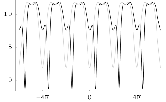
Figure 1: Periodic first-order SUSY partner potential $\widetilde{V}_{+}(x)$ (black curve) isospectral to the associated Lamé potential (gray curve) with $m=3,\ \ell=1$, $k^{2}=0.95$, generated by using the Bloch solution $u(x)=\psi^{+}(x)$ with $\epsilon=4.75$.

4 Applications

In a previous paper [7] we have found solutions of the stationary Schrödinger equation with an arbitrary energy (either physical or non-physical) for the associated Lamé potentials, the pair $(m,\ell)$ taking the values $(1,1)$ and $(2,1)$. We applied there also the first-order SUSY techniques in order to generate new potentials with known spectra. Here, we will illustrate our previous general results with a different case characterized by $(m,\ell)=(3,1)$. For this associated Lamé potential explicit expressions for some band-edge eigenfunctions and eigenvalues are known [3]:

$$\psi_{(1)}={\rm cn}\,x\,{\rm dn}^{2}x,\hskip 56.9055ptE_{1}=1+4k^{2},$$

$$\psi_{(2)}={\rm sn}\,x\,{\rm dn}^{2}x,\hskip 56.9055ptE_{2}=1+9k^{2},$$

$$\psi_{(3,8)} = \frac{{\rm sn}\,x\,{\rm cn}\,x}{{\rm dn}\,x}\left[{\rm sn}^{2}x-\frac{1}{5k^{2}}\left(k^{2}+3\pm\sqrt{k^{4}-9k^{\prime 2}}\right)\right],$$

$$E_{3,8} = 10+2k^{2}\mp 2\sqrt{k^{4}-9k^{\prime 2}}.$$

Three other band edge eigenfunctions can be given:

$$\hskip-28.45274pt\psi_{(i)}=\frac{{\rm sn}^{4}x}{{\rm dn}\,x}-\frac{(9k^{2}+16-E_{i})}{10k^{2}}\frac{{\rm sn}^{2}x}{{\rm dn}\,x}+\frac{E_{i}^{2}-2(5k^{2}+18)E_{i}+9k^{4}+156k^{2}+320}{15k^{4}{\rm dn}\,x}$$

where the eigenvalues $E_{i},\ i=0,4,7$ are the ordered roots of the cubic equation:

$$E^{3}-(11k^{2}+20)E^{2}+(19k^{4}+216k^{2}+64)E-(9k^{6}+388k^{4}+448k^{2})=0$$

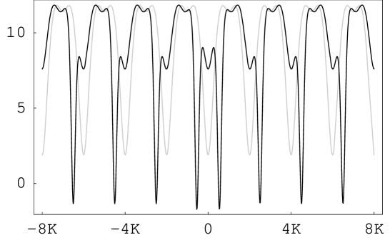
Figure 2: Non-periodic first-order SUSY partner $\widetilde{V}^{np}(x)$ (black curve) of the associated Lamé potential (gray curve) for $m=3,\ \ell=1$, $k^{2}=0.95$, which was generated by using $u(x)=\psi^{+}(x)+\psi^{-}(x)$ with $\epsilon=4.75$. The new Hamiltonian $\widetilde{H}^{np}$ has an extra bound state precisely at $\epsilon=4.75$.

Our first task is to evaluate four constants $a_{1},a_{2},a_{3},a_{4}$ (note that $m+\ell=4$) in (23), where without loss of generality, we choose $a_{0}=1$. Let us first write down the basic elements $f_{i}$ for $m=3,\ell=1$ from (11-13)

$$\hskip-14.22636ptf_{0}(\rho)=\bar{e}_{3}\rho(\rho-3)(2\rho-3),\quad f_{1}(\rho)=2(\rho-1)\{3e_{1}[4-(\rho-1)^{2}]-\widetilde{E}\},$$ (69)

$$f_{2}(\rho)=\bar{e}_{2}(\rho-4)(\rho+3)(2\rho-1),\qquad\widetilde{E}=\bar{e}_{3}(E-2)+12e_{3}.$$ (70)

Note that the two constants $a_{1},a_{2}$ have to be determined from (15)

$$a_{1}=-\frac{F_{1}}{f_{0}(1)},\qquad a_{2}=\frac{F_{2}}{f_{0}(1)f_{0}(2)},$$ (71)

while the remaining two are to be computed from (22)

$$a_{3}=-\frac{D_{1}f_{2}(2)}{D_{2}}a_{2},\qquad a_{4}=\frac{D_{0}f_{2}(2)f_{2}(3)}{D_{2}}.$$ (72)

Now from (16), one may write quite straightforwardly the $F_{i}$’s

$$F_{1}=f_{1}(0),\qquad F_{2}=\left|\begin{array}[]{ll}f_{1}(1)&f_{2}(0)\\ f_{0}(1)&f_{1}(0)\end{array}\right|,$$ (73)

and to obtain the $D_{i}$’s we need

$$F_{5}=\left|\begin{array}[]{lllll}f_{1}(4)&f_{2}(3)&\hskip 19.91684pt0&\hskip 19.91684pt0&\hskip 19.91684pt0\\ f_{0}(4)&f_{1}(3)&f_{2}(2)&\hskip 19.91684pt0&\hskip 19.91684pt0\\ \hskip 19.91684pt0&f_{0}(3)&f_{1}(2)&f_{2}(1)&\hskip 19.91684pt0\\ \hskip 19.91684pt0&\hskip 19.91684pt0&f_{0}(2)&f_{1}(1)&f_{2}(0)\\ \hskip 19.91684pt0&\hskip 19.91684pt0&\hskip 19.91684pt0&f_{0}(1)&f_{1}(0)\\ \end{array}\right|.$$ (74)

Then the final quantities are

$$D_{0}=[\mbox{minor of $F_{5}$ in $F_{5}$}]=1,$$ (75)

$$D_{1}=[\mbox{minor of $F_{4}$ in $F_{5}$}]=f_{1}(4),$$ (76)

$$D_{2}=[\mbox{minor of $F_{3}$ in $F_{5}$}]=\left|\begin{array}[]{ll}f_{1}(4)&f_{2}(3)\\ f_{0}(4)&f_{1}(3)\end{array}\right|.$$ (77)

Finally, using the ingredients (69-77) we obtain

$$a_{0}=1,\qquad a_{1}=\frac{9e_{1}-\widetilde{E}}{\bar{e}_{3}},\qquad a_{2}=\frac{6\bar{e}_{2}}{\bar{e}_{3}},$$

$$a_{3}=-\frac{45(\widetilde{E}+15e_{1})\bar{e}_{2}^{2}}{(\widetilde{E}^{2}+15e_{1}\widetilde{E}+25\bar{e}_{2}\bar{e}_{3})\bar{e}_{3}},\quad a_{4}=\frac{225\,\bar{e}_{2}^{3}}{(\widetilde{E}^{2}+15e_{1}\widetilde{E}+25\bar{e}_{2}\bar{e}_{3})\bar{e}_{3}}.$$ (78)

We employ these coefficients then to find the roots $c_{r},r=1,\dots,4$ of the fourth-order equation

$$\sum_{r=0}^{4}a_{r}\left(\frac{e_{1}-t}{\bar{e}_{2}}\right)^{r}=0,$$ (79)

which can be analytically determined, but their explicit expression is too involved to be shown here. These roots are used then to invert the transcendental equation $\wp(b_{r})=c_{r}$ to determine the $b_{r}$’s (with the restriction $\Psi^{\prime}|_{z=b_{r}}>0$), which are thus inserted in the explicit expressions for $\psi^{\pm}(x)$. Finally, the resulting Bloch solutions can be used, either directly or in the corresponding Wronskian, to derive the periodic SUSY partner potentials $\widetilde{V}_{\pm}(x)$ of (54) or $\widetilde{V}(x)$ of (62). On the other hand, different linear combinations of kind (55) or (63) can be used to derive the potentials $\widetilde{V}^{np}(x)$ of (57) or (68) which have periodicity defects. The final results of these procedures are illustrated in figures below. In the four figures we show in gray the original associated Lamé potential for $m=3$, $\ell=1$, $k^{2}=0.95$. In figure 1 we show as well in black one of its periodic first-order SUSY partners generated through a Bloch solution with $\epsilon=4.75$ while in Figure 2 it is illustrated one of its non-periodic partners for the same $\epsilon$, which is lesser than but close to the lowest band edge $E_{0}=4.79991$. On the other hand, in figures 3 and 4 we have drawn similar graphs (black curves) for the corresponding second-order SUSY partners, periodic and non-periodic respectively. For the periodic case (Figure 3) we have used two Bloch solutions $u_{1}(x)=\psi_{1}^{+}(x)$, $u_{2}(x)=\psi_{2}^{+}(x)$ associated to the pair of factorization energies $\epsilon_{1}=9.4$, and $\epsilon_{2}=9.5$ which are in the first finite energy gap $(4.8,9.55)$. For the non-periodic case we have used the same pair of factorization energies, with linear combinations $u_{1}(x)=\psi_{1}^{+}(x)+\psi_{1}^{-}(x)$ and $u_{2}(x)=\psi_{2}^{+}(x)-2\psi_{2}^{-}(x)$. In both non-periodic cases the periodicity defects are clearly detected.

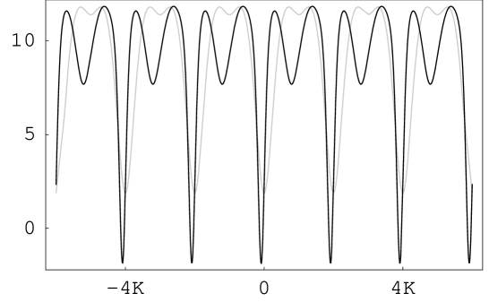
Figure 3: Periodic second-order SUSY partner potential $\widetilde{V}(x)$ (black curve) isospectral to the associated Lamé potential (gray curve) with $m=3,\ \ell=1$, $k^{2}=0.95$, generated by using $\epsilon_{1}=9.4$, $u_{1}(x)=\psi_{1}^{+}(x)$ and $\epsilon_{2}=9.5$, $u_{2}(x)=\psi_{2}^{+}(x)$.

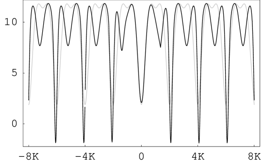
Figure 4: Non-periodic second-order SUSY partner $\widetilde{V}^{np}(x)$ (black curve) of the associated Lamé potential (gray curve) with $m=3,\ \ell=1$, $k^{2}=0.95$, which was generated by using $\epsilon_{1}=9.4$, $u_{1}(x)=\psi_{1}^{+}(x)+\psi_{1}^{-}(x)$ and $\epsilon_{2}=9.5$, $u_{2}(x)=\psi_{2}^{+}(x)-2\psi_{2}^{-}(x)$. The Hamiltonian $\widetilde{H}^{np}$ has the same band spectrum as the initial associated Lamé potential plus two isolated bound states at $\epsilon_{1}$ and $\epsilon_{2}$.

5 Conclusions

In this article we have shown, by finding explicitly the two solutions of Bloch type associated to the stationary Schrödinger equation for an arbitrary value of the energy, that the associated Lamé potentials for any integer values of the parameter pairs $(m,\ell)$ are exactly solvable. This point is clarifying because in most of the works concerning Schrödinger equation with periodic potentials typically one looks for just the band edge eigenfunctions, thus inducing the idea that these solutions are the only ones which could be analytically determined. The solved problem is very important for implementing the supersymmetric transformations, of first or higher order, since the non-physical Schrödinger solutions can be used as seeds to generate new exactly solvable potentials. Consequently, we have generated in this way potentials which are either strictly isospectral to the initial one or with some isolated bound states embedded at the energy gaps of the initial Hamiltonian. The arising of these two different kinds of spectra for the new potentials depends on either we choose as seeds directly the Bloch solutions or general linear combinations for the chosen factorization energies. The potentials with bound states embedded into the finite gaps may be interesting for physical applications since the corresponding levels could work as auxiliary transition energies for the electron to jump easier between allowed bands.

Appendix A Appendix

In the following we will provide a short introduction about elliptic functions (for more details, see [28, 29]). Three Jacobian elliptic functions are defined by

$${\rm sn}(x,k)=\sin\varphi,\quad{\rm cn}(x,k)=\cos\varphi,\quad{\rm dn}(x,k)=d\varphi/dx,$$ (80)

where amplitude function $\varphi(z,k)$ is defined by the integral

$$z(\varphi,k)=\int_{0}^{\varphi}\frac{d\tau}{\sqrt{1-k^{2}\sin^{2}\tau}}.$$ (81)

The square of the real number $k$ is called elliptic modulus parameter and $k^{2}\in(0,1)$. $k^{\prime 2}=1-k^{2}$ is called complementary modulus parameter. For simplicity, in the text we suppress the explicit modular dependence and write ${\rm sn}\,x,\ {\rm cn}\,x,\ {\rm dn}\,x$, etc. These are doubly periodic functions of periods $4K,2iK^{\prime}$; $4K,4iK^{\prime}$ and $2K,4iK^{\prime}$ respectively, where the quarter-periods $K$ and $K^{\prime}$ are the real numbers given by

$$K(k)\equiv K=z(\pi/2,k),\qquad K^{\prime}(k)\equiv K^{\prime}=K(k^{\prime}).$$ (82)

$K$ is called complete elliptic integral of second kind. Some relevant relations are

$${\rm sn}(x+K)=\frac{{\rm cn}\,x}{{\rm dn}\,x},\quad{\rm cn}(x+K)=-k^{\prime}\frac{{\rm sn}\,x}{{\rm dn}\,x},\quad{\rm dn}(x+K)=\frac{k^{\prime}}{{\rm dn}\,x},$$ (83)

$${\rm sn}(x+2K)=-{\rm sn}\,x,\quad{\rm cn}(x+2K)=-{\rm cn}\,x,\quad{\rm dn}(x+2K)={\rm dn}\,x,$$ (84)

$${\rm sn}(x+iK^{\prime})=\frac{1}{k{\rm sn}\,x},\quad{\rm cn}(x+iK^{\prime})=-\frac{i}{k}\frac{{\rm dn}\,x}{{\rm sn}\,x},\quad{\rm dn}(x+iK^{\prime})=-i\frac{{\rm cn}\,x}{{\rm sn}\,x},$$ (85)

$${\rm sn}^{2}x+{\rm cn}^{2}x=1,\qquad{\rm dn}^{2}x+k^{2}{\rm sn}^{2}x=1,$$ (86)

and the rules of differentiation are

$${\rm sn}^{\prime}x={\rm cn}\,x\ {\rm dn}\,x,\quad{\rm cn}^{\prime}x=-{\rm sn}\,x\ {\rm dn}\,x,\quad{\rm dn}^{\prime}x=-k^{2}{\rm sn}\,x\ {\rm cn}\,x.$$ (87)

Weierstrass elliptic function $\wp(z;g_{2},g_{3})\equiv\wp(z)$ is defined by

$$\wp(z)=\frac{1}{z^{2}}+\sum_{m,n}^{{}^{\prime}}\left[\frac{1}{(z-2m\omega-2n\omega^{\prime})^{2}}-\frac{1}{(2m\omega+2n\omega^{\prime})^{2}}\right],$$ (88)

where the symbol $\sum^{\prime}$ means summation over all integer values of $m,n$ except $m=n=0$; $\omega,\ \omega^{\prime}$ being half-periods of $\wp(z)$. The invariants $g_{2},g_{3}$ are given by

$$g_{2}=60\sum_{m,n}^{{}^{\prime}}\frac{1}{(m\omega+n\omega^{\prime})^{4}},\qquad g_{3}=140\sum_{m,n}^{{}^{\prime}}\frac{1}{(m\omega+n\omega^{\prime})^{6}}\,.$$ (89)

The three numbers $e_{i},i=1,2,3$ are defined by $\wp(\omega_{i})=e_{i}$, where $\omega_{1}\equiv\omega,\ \omega_{3}\equiv\omega^{\prime}$ and $\omega_{2}=\omega+\omega^{\prime}$. To get the relation between Jacobian elliptic functions and Weierstrass elliptic function, it is necessary to define $\omega,\omega^{\prime}$ in terms of $K,K^{\prime}$. We have taken the following definition

$$\omega=\frac{K}{\sqrt{\bar{e}_{3}}},\qquad\omega^{\prime}=\frac{iK^{\prime}}{\sqrt{\bar{e}_{3}}},$$ (90)

which corresponds to the case when the discriminant $\Delta=g_{2}^{3}-27g_{3}^{2}>0$. This means that the numbers $e_{i}$ are always real and consequently they can be ordered as $e_{1}>e_{2}>e_{3}$, because these are roots of the equation

$$4t^{3}-g_{2}t-g_{3}=0.$$ (91)

The relations between $\wp(z)$ and ${\rm sn}\,z,\ {\rm cn}\,z,\ {\rm dn}\,z$ may then be written as

$$\wp\left(\frac{z}{\sqrt{\bar{e}_{3}}}\right)=e_{1}+\bar{e}_{3}\frac{{\rm cn}^{2}z}{{\rm sn}^{2}z}=e_{2}+\bar{e}_{3}\frac{{\rm dn}^{2}z}{{\rm sn}^{2}z}=e_{3}+\bar{e}_{3}\frac{1}{{\rm sn}^{2}z}.$$ (92)

It may be mentioned that the derivative of $\wp(z)$ is also an elliptic function with same periods and satisfy the relation

$$\wp^{\prime 2}(z)=4\>\prod^{3}_{i=1}\left[\wp(z)-e_{i}\right].$$ (93)

It is now straightforward to obtain equation (3) from equation (1) under the translation $x=\sqrt{\bar{e}_{3}}z+iK^{\prime}$ by using the relations (85) and (92). We will now apply the transformation $y=(e_{1}-\wp(z))/\bar{e}_{2}$ on equation (5). Noting the following relations

$$\wp^{\prime\prime}(z)=6\wp^{2}(z)-\frac{g_{2}}{2},\qquad\frac{\wp^{\prime\prime\prime}(z)}{\wp^{\prime}(z)}=12\wp(z),$$ (94)

it is not very difficult to obtain the following equation

$$2\prod^{3}_{i=1}\big{[}\wp(z)-e_{i}\big{]}\frac{d^{3}\Psi}{dy^{3}}-3\bigg{[}3\wp^{2}(z)+\sum^{3}_{\begin{array}[]{c}{\scriptstyle i,j=1}\\ {\scriptstyle i\neq j}\end{array}}e_{i}e_{j}\bigg{]}\bar{e}_{2}\frac{d^{2}\Psi}{dy^{2}}$$ (97)

$$+2\bigg{\{}[3-m(m+1)]\wp(z)-\frac{\ell(\ell+1)\bar{e}_{2}\bar{e}_{3}}{\wp(z)-e_{1}}+\widetilde{E}\bigg{\}}(\bar{e}_{2})^{2}\frac{d\Psi}{dy}$$

$$+\bigg{\{}m(m+1)-\frac{\ell(\ell+1)\bar{e}_{2}\bar{e}_{3}}{[\wp(z)-e_{1}]^{2}}\bigg{\}}(\bar{e}_{2})^{3}\Psi=0$$ (98)

The equation (7) will then readily follow under the transformation $\Phi(y)=[\wp(z)-e_{1}]^{\ell}\Psi$ on above equation by using the relations (94).

References

• [1] A. Khare, U. Sukhatme, J. Math. Phys. 40 (1999) 5473; ibid 42 (2001) 5652.
• [2] A. Ganguly, Mod. Phys. Lett. A 15 (2000) 1923 (math-ph/0204026).
• [3] A. Ganguly, J. Math. Phys. 43 (2002) 1980 (math-ph/0207028); ibid 43 (2002) 5310 (math-ph/0212045).
• [4] G.V. Dunne, M. Shifman, Ann. Phys. 299 (2002) 143.
• [5] V.M. Tkachuk, O. Voznyak, Phys. Lett. A 301 (2002) 177.
• [6] S.S. Ranjani, A.K. Kapoor, P.K. Panigrahi, Mod. Phys. Lett. A 19 (2004) 2047.
• [7] D.J. Fernández, A. Ganguly, Phys. Lett. A 338 (2005) 203.
• [8] A.D. Alhaidari, Ann. Phys. 317 (2005) 152.
• [9] B.K. Bagchi, Supersymmetry in Quantum and Classical Mechanics, Chapman and Hall, Boca Raton, Florida (2000).
• [10] I. Aref’eva, D.J. Fernández, V. Hussin, J. Negro, L.M. Nieto, B.F. Samsonov, Special issue dedicated to the subject of the International Conference on Progress in supersymmetric quantum mechanics, J. Phys. A 37, Number 43 (2004).
• [11] B. Mielnik, O. Rosas-Ortiz, J. Phys. A 37 (2004) 10007.
• [12] J. Negro, L.M. Nieto, O. Rosas-Ortiz, J. Phys. A 37 (2004) 10079.
• [13] A.A. Andrianov, F. Cannata, J. Phys. A 37 (2004) 10297.
• [14] M.V. Ioffe, J. Phys. A 37 (2004) 10363.
• [15] C.V. Sukumar, AIP Conference Proceedings 744 (2005) 166.
• [16] D.J. Fernández, N. Fernández-García, AIP Conference Proceedings 744 (2005) 236 (quant-ph/0502098).
• [17] G. Dunne, J. Feinberg, Phys. Rev. D 57 (1998) 1271.
• [18] D.J. Fernández, J. Negro, L.M. Nieto, Phys. Lett. A 275 (2000) 338.
• [19] J. Negro, L.M. Nieto, D.J. Fernández, Czech. J. Phys. 50 (2000) 1303.
• [20] D.J. Fernández, B. Mielnik, O. Rosas-Ortiz, B.F. Samsonov, J. Phys. A 35 (2002) 4279 (quant-ph/0303051).
• [21] D.J. Fernández, B. Mielnik, O. Rosas-Ortiz, B.F. Samsonov, Phys. Lett. A 294 (2002) 168 (quant-ph/0302204).
• [22] O. Rosas-Ortiz, Rev. Mex. Fís. 49 S2 (2003) 145 (quant-ph/0302198).
• [23] B. Bagchi, A. Ganguly, D. Bhaumik, A. Mitra, Mod. Phys. Lett. A 14 (1999) 27.
• [24] A. Gonzalez-Lopez, T. Tanaka, Phys. Lett. B 586 (2004) 117.
• [25] E.L. Ince, Ordinary Differential Equations, Dover Publications, New York (1956).
• [26] E.T. Whittaker, G.N. Watson, A course of modern analysis, Cambridge University Press, Cambridge (1963).
• [27] L. Trlifaj, Inv. Prob. 5 (1989) 1145.
• [28] I.S. Gradshteyn, I.M. Ryzhik, Tables of Integrals, Series and Products, Academic Press, New York, (1965).
• [29] M. Abramowitz, I.A. Stegun (Editors), Handbook of Mathematical Functions, Dover Publications, INC, New York (1965).